Clim. Past, 9, 1111–1140, 2013 www.clim-past.net/9/1111/2013/ doi:10.5194/cp-9-1111-2013
© Author(s) 2013. CC Attribution 3.0 License.
EGU Journal Logos (RGB)
Advances in
Geosciences
Open Access
Natural Hazards
and Earth System
Sciences
Open Access
Annales
Geophysicae
Open Access
Nonlinear Processes
in Geophysics
Open Access
Atmospheric
Chemistry
and Physics
Open Access
Atmospheric
Chemistry
and Physics
Open Access
Discussions
Atmospheric
Measurement
Techniques
Open Access
Atmospheric
Measurement
Techniques
Open Access
Discussions
Biogeosciences
Open Access Open Access
Biogeosciences
Discussions
Climate
of the Past
Open Access Open Access
Climate
of the Past
Discussions
Earth System
Dynamics
Open Access Open Access
Earth System
Dynamics
Discussions
Geoscientific
Instrumentation
Methods and
Data Systems
Open Access
Geoscientific
Instrumentation
Methods and
Data Systems
Open Access
Discussions
Geoscientific
Model Development
Open Access Open Access
Geoscientific
Model Development
Discussions
Hydrology and
Earth System
Sciences
Open Access
Hydrology and
Earth System
Sciences
Open Access
Discussions
Ocean Science
Open Access Open Access
Ocean Science
DiscussionsSolid Earth
Open Access Open Access
Solid Earth
Discussions
The Cryosphere
Open Access Open Access
The Cryosphere
Discussions
Natural Hazards
and Earth System
Sciences
Open Access
Discussions
Historical and idealized climate model experiments: an
intercomparison of Earth system models of intermediate complexity
M. Eby1, A. J. Weaver1, K. Alexander1, K. Zickfeld2, A. Abe-Ouchi3,4, A. A. Cimatoribus5, E. Crespin6,
S. S. Drijfhout5, N. R. Edwards7, A. V. Eliseev8, G. Feulner9, T. Fichefet6, C. E. Forest10, H. Goosse6, P. B. Holden7,
F. Joos11,12, M. Kawamiya4, D. Kicklighter13, H. Kienert9, K. Matsumoto14, I. I. Mokhov8, E. Monier15, S. M. Olsen16,
J. O. P. Pedersen17, M. Perrette9, G. Philippon-Berthier6, A. Ridgwell18, A. Schlosser15, T. Schneider von Deimling9,
G. Shaffer19,20, R. S. Smith21, R. Spahni11,12, A. P. Sokolov15, M. Steinacher11,12, K. Tachiiri4, K. Tokos14,
M. Yoshimori3, N. Zeng22, and F. Zhao22
1School of Earth and Ocean Sciences, University of Victoria, Victoria, British Columbia, Canada 2Simon Fraser University, Vancouver, British Columbia, Canada
3Atmosphere and Ocean Research Institute, The University of Tokyo, Kashiwa, Japan
4Research Institute for Global Change, Japan Agency for Marine-Earth Science and Technology, Yokohama, Japan 5Royal Netherlands Meteorological Institute, De Bilt, the Netherlands
6Georges Lemaˆıtre Centre for Earth and Climate Research, Universit´e Catholique de Louvain, Louvain-La-Neuve, Belgium 7The Open University, Milton Keynes, UK
8A. M. Obukhov Institute of Atmospheric Physics, RAS, Moscow, Russia 9Potsdam Institute for Climate Impact Research, Potsdam, Germany 10Pennsylvania State University, Pennsylvania, USA
11Climate and Environmental Physics, Physics Institute, University of Bern, Bern, Switzerland 12Oeschger Centre for Climate Change Research, University of Bern, Bern, Switzerland 13The Ecosystems Center, MBL, Woods Hole, Massachusetts, USA
14University of Minnesota, Minneapolis, Minnesota, USA
15Massachusetts Institute of Technology, Cambridge, Massachusetts, USA 16Danish Meteorological Institute, Copenhagen, Denmark
17National Space Institute, Technical University of Denmark, Kgs. Lyngby, Denmark 18School of Geographical Sciences, University of Bristol, Bristol, UK
19Department of Geophysics, University of Concepcion, Concepcion, Chile 20Niels Bohr Institute, University of Copenhagen, Copenhagen, Denmark
21National Centre for Atmospheric Science – Climate, University of Reading, Reading, UK 22University of Maryland, College Park, Maryland, USA
Correspondence to: M. Eby ([email protected])
Received: 27 July 2012 – Published in Clim. Past Discuss.: 28 August 2012 Revised: 8 March 2013 – Accepted: 13 March 2013 – Published: 16 May 2013
Abstract. Both historical and idealized climate model
ex-periments are performed with a variety of Earth system mod-els of intermediate complexity (EMICs) as part of a commu-nity contribution to the Intergovernmental Panel on Climate Change Fifth Assessment Report. Historical simulations start at 850 CE and continue through to 2005. The standard sim-ulations include changes in forcing from solar luminosity,
Earth’s orbital configuration, CO2, additional greenhouse
fluxes, and recent land fluxes appear to be slightly under-estimated. It is possible that recent modelled climate trends or climate–carbon feedbacks are overestimated resulting in too much land carbon loss or that carbon uptake due to CO2and/or nitrogen fertilization is underestimated. Several
one thousand year long, idealized, 2×and 4×CO2
exper-iments are used to quantify standard model characteristics, including transient and equilibrium climate sensitivities, and climate–carbon feedbacks. The values from EMICs gener-ally fall within the range given by general circulation models. Seven additional historical simulations, each including a sin-gle specified forcing, are used to assess the contributions of different climate forcings to the overall climate and carbon cycle response. The response of surface air temperature is the linear sum of the individual forcings, while the carbon cy-cle response shows a non-linear interaction between land-use change and CO2forcings for some models. Finally, the
prein-dustrial portions of the last millennium simulations are used to assess historical model carbon-climate feedbacks. Given the specified forcing, there is a tendency for the EMICs to underestimate the drop in surface air temperature and CO2
between the Medieval Climate Anomaly and the Little Ice Age estimated from palaeoclimate reconstructions. This in turn could be a result of unforced variability within the cli-mate system, uncertainty in the reconstructions of tempera-ture and CO2, errors in the reconstructions of forcing used to
drive the models, or the incomplete representation of certain processes within the models. Given the forcing datasets used in this study, the models calculate significant land-use emis-sions over the pre-industrial period. This implies that land-use emissions might need to be taken into account, when making estimates of climate–carbon feedbacks from palaeo-climate reconstructions.
1 Introduction
Climate models are powerful tools that help us to under-stand how climate has changed in the past and how it may change in the future. Climate models vary in com-plexity from highly parameterized box models to sophisti-cated Earth system models with coupled atmosphere–ocean general circulation model (AOGCM) subcomponents, such as those involved in the Coupled Model Intercomparison Project Phase 5 (CMIP5; Taylor et al., 2012). Different mod-els are designed to address different scientific questions. Simple models are often useful in developing and under-standing individual processes and feedbacks, or teasing apart the basic physics of complex systems. However, they usually lack the complex interactions that are an integral part of the climate system. Current “state-of-the-art” Earth system mod-els are both sophisticated and complex, but the number and length of simulations that can be performed is limited by the availability of computing resources. Another class of models, known as Earth system models of intermediate complexity
(EMICs), helps fill the gap between the simplest and the most complex climate models (Claussen et al., 2002).
Usually EMICs are complex enough to capture essential climate processes and feedbacks while compromising on the complexity of one or more climate model component. Often EMICs are used at lower resolution, and model components may have reduced dimensionality. While generally simpler, EMICs sometimes include more subcomponent models than Earth system AOGCMs. New subcomponents (for example, continental ice sheets, representations of peatlands, wetlands or permafrost) are often developed within the EMIC frame-work before they are embedded into coupled AOGCMs, be-cause development and testing is less computationally expen-sive. In addition, there are some processes operating within the Earth system (e.g. carbonate dissolution from sediments or chemical weathering) with very long inherent timescales that can only be integrated by EMICs.
With relatively abundant proxy data, the last millennium is an important test bed for validating the longer term climate– carbon response of models. Understanding the role of climate forcing over this period will help to reconcile any inconsis-tences between the models and the various palaeo-forcing and data reconstructions and improve our confidence in fu-ture simulations. There are a very limited number of stud-ies that have modelled the climate–carbon cycle response over this period (Gerber et al., 2003; Goosse et al., 2010; Jungclaus et al., 2010), and while a few AOGCMs have carried out climate simulations over the last millennium (for example, Gonz´alez-Rouco et al., 2003; Jungclaus et al., 2010; Swingedouw et al., 2010; and Fern´andez-Donado et al., 2012), these studies were limited in the number of ex-periments that could be performed. See Fern´andez-Donado et al. (2012) for a comprehensive review of the current state of climate simulation and reconstruction over the last millennium.
Given their relatively rapid integration times, EMICs are capable of simulating climate change over many thousands of years. They are able to perform the many simulations needed to investigate the sensitivity of climate to various ex-ternal forcings. EMICs often have relatively low levels of internal variability, which makes them particularly useful in experiments investigating the forced response of the climate system. Many EMICs also include long timescale carbon processes such as changes in carbonate sedimentation, wet-lands or permafrost, processes which are usually missing in models designed for shorter simulations. These characteris-tics make EMICs particularly well suited to investigate the forced climate–carbon response over the last millennium.
were used extensively in the Intergovernmental Panel on Climate Change (IPCC) Fourth Assessment Report (AR4; IPCC, 2007). As part of the EMIC community’s contribution to the Fifth Assessment Report, 15 EMICs have contributed results from a series of experiments designed to examine cli-mate change over the last millennium and to extend the rep-resentative concentration pathways projections that are being simulated by the CMIP5 models.
This paper summarizes the results of historical and ide-alized experiments. The climate and carbon cycle response of models over the historical period are compared to obser-vational estimates. Idealized experiments are used to gener-ate climgener-ate and carbon cycle metrics for comparison with previous studies or results from other models. The histori-cal climate response is presented in Sect. 3.1 and idealized climate metrics in Sect. 3.2. The historical carbon response is discussed in Sect. 3.3 and idealized carbon metrics in Sect. 3.4. Historical experiments that were used to explore the contributions of various specified forcings over the last millennium are described in Sect. 3.5 and the linearity of the response in Sect. 3.6. Contributions of natural and an-thropogenic forcings to the climate response are compared in Sect. 3.7. The preindustrial portion of the last millennium is also used to assess changes in temperature in Sect. 3.8, changes in CO2 in Sect. 3.9, and the climate–carbon cycle
sensitivity in Sect. 3.10. Details of experiments that explore future climate change commitment and irreversibility can be found in Zickfeld et al. (2013).
2 Experimental design
2.1 Models
Fifteen EMICs participated in this intercomparison project. The participating model names with version numbers, fol-lowed by a two-letter abbreviation (in parentheses), and con-tributing institution, are as follows: Bern3D (B3) from the University of Bern; CLIMBER-2.4 (C2) from the Potsdam Institute for Climate Impact Research; CLIMBER-3α (C3) from the Potsdam Institute for Climate Impact Research; DCESS v1 (DC) from the Danish Center for Earth System Science; FAMOUS vXFXWB (FA) from the University of Reading; GENIE release 2-2-7 (GE) from The Open Uni-versity; IAP RAS CM (IA) from the Russian Academy of Sciences; IGSM v2.2 (I2) from the Massachusetts Institute of Technology; LOVECLIM v1.2 (LO) from the Univer-sit´e Catholique de Louvain; MESMO v1.0 (ME) from the University of Minnesota; MIROC-lite (MI) from the Uni-versity of Tokyo; MIROC-lite-LCM (ML) from the Japan Agency for Marine-Earth Science and Technology; SPEEDO (SP) from the Royal Netherlands Meteorological Institute; UMD v2.0 (UM) from the University of Maryland; and UVic v2.9 (UV) from the University of Victoria. Model characteristics are compared in Table 1, and more complete
descriptions are provided in Appendix A. Unlike the EMICs cited in the AR4, several models now calculate land-use change carbon fluxes internally (B3, DC, GE, I2, ML, UV) and/or include ocean sediment and terrestrial weathering (B3, DC, GE, UV). Eight EMICs (B3, DC, GE, I2, ME, ML, UM and UV) include interactive land and ocean carbon cy-cle components that allow them to diagnose emissions that are compatible with specified CO2concentrations.
2.2 Methods
To be consistent with other intercomparison projects, forc-ing for the initial condition and the historical period were obtained from the Paleoclimate Modelling Intercompari-son Project Phase 3 (PMIP3) and CMIP5-recommended datasets. Specified forcings included orbital configuration (from Berger, 1978), trace gases from various ice cores (Schmidt et al., 2012; Meinshausen et al., 2011), volcanic aerosols (Crowley et al., 2008), solar irradiance (Delaygue and Bard, 2009; Wang et al., 2005), sulphate aerosols (Lamarque et al., 2010) and land use (Pongratz et al., 2008; Hurtt et al., 2011). The warming from black carbon and the indirect effect of ozone, and the cooling from the indi-rect effect of sulphate aerosols were not included. Forcing data from PMIP3 and CMIP5 were concatenated or linearly blended before 1850 when necessary. From 1850 to 2005, all specified forcings are identical to the historical portion of the Representative Concentration Pathway (RCP) scenarios. See Appendix B for details on the implementation of the forcing protocol and how this may differ between models. All years in this paper are given as Common Era (CE) unless stated otherwise.
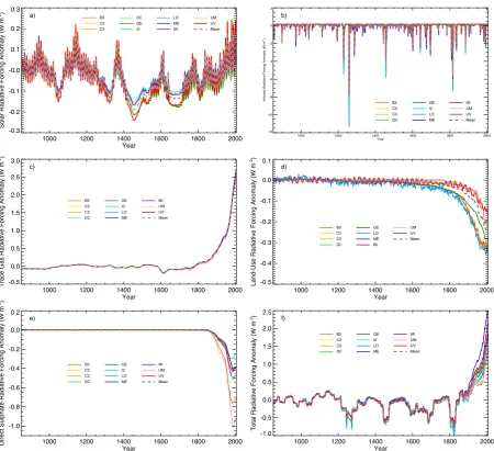
Diagnosed model equivalent radiative forcing estimates, for the various specified external forcings, are shown in Fig. 1. Given the large diversity of EMICs, not all models are able to apply the specified forcing in the same way. Some diagnosed estimates of equivalent radiative forcing are only approximate. This is especially true for sulphate aerosol and land-use forcing, which are more complex to implement and diagnose than most of the other externally specified forcings. The multi-model mean radiative forcing estimates for the di-rect effect of trace gases, sulphates and land-use change are very similar to estimates from the Task Group: RCP Concen-trations Calculation and Data (Meinshausen et al., 2011), and present-day estimates are similar to those given in the AR4 (Forster et al., 2007). The ranges in diagnosed radiative forc-ing in Fig. 1 are also similar to the ranges from the models described by Fern´andez-Donado et al. (2012), with most of the variation between models due to the implementation of anthropogenic forcing (which includes aerosols and land-use change).
1000 1200 1400 1600 1800 2000 Year
-0.3 -0.2 -0.1 -0.0 0.1 0.2 0.3
Solar Radiative Forcing Anomaly (W m
-2) B3
C2 C3
DC GE I2
LO ME MI
UM UV Mean
a)
1000 1200 1400 1600 1800 2000
Year -0.5
0.0 0.5 1.0 1.5 2.0 2.5 3.0
Trace Gas Radiative Forcing Anomaly (W m
-2)
B3 C2 C3 DC
GE I2 LO ME
MI UM UV Mean
c)
1000 1200 1400 1600 1800 2000
Year -1.0
-0.8 -0.6 -0.4 -0.2 0.0 0.2
Direct Sulphate Radiative Forcing Anomaly (W m
-2)
B3 C2 C3 DC
GE I2 LO ME
MI UM UV Mean
e)
1000 1200 1400 1600 1800 2000
Year -1.0
-0.5 0.0 0.5 1.0 1.5 2.0 2.5
Total Radiative Forcing Anomaly (W m
-2)
B3 C2 C3 DC
GE I2 LO ME
MI UM UV Mean
f)
1000 1200 1400 1600 1800 2000
Year -12
-10 -8 -6 -4 -2 0 2
Volcanic Radiative Forcing Anomaly (W m
-2)
B3 C2 C3 DC
GE I2 LO ME
MI UM UV Mean
b)
1000 1200 1400 1600 1800 2000
Year -0.5
-0.4 -0.3 -0.2 -0.1 0.0 0.1
Land-Use Radiative Forcing Anomaly (W m
-2)
B3 C2 C3 DC
GE LO ME MI
UM UV Mean
d)
Fig. 1. Annual average radiative forcing estimates, from specified forcing changes in the historical simulations, for 11 of the participating
models. Changes in radiative forcing from changes in solar irradiance are shown in (a), volcanic aerosols in (b), greenhouse gases in (c), land use in (d), the direct effect of sulphate aerosols in (e), and all forcings in (f). Due to the complexity of implementing forcing from land use and the direct effects of sulphate aerosols in some models, the diagnosed radiative forcing estimates should be considered to be only approximate. Models that specified equivalent task group radiative forcings may be exactly overplotted and appear to be missing (see Appendix B for details on forcing). Land-use radiative forcing was not available for model I2. Radiative forcing is plotted as an anomaly of the multi-model mean over the century centred at year 900. Forcing estimates in panels (a) to (e) are unfiltered while the results in (f) have been processed with a 30 yr moving average, rectangular filter. Changes in radiative forcing due to changes in orbit are much smaller than any of the other forcings and are not shown separately, but they are included in the total radiative forcing shown in (f).
from the year 850, but the B3 model started from equilibrium at the Last Glacial Maximum in order to ensure that its per-mafrost and peatland components were in a consistent initial state by the year 850.
Models were then integrated to the year 2005 under var-ious specified transient forcings. Nine historical simula-tions with specified CO2 concentrations were performed.
Seven simulations specified only one of the following tran-sient forcings: non-CO2 trace gases, CO2, land use, solar
luminosity, orbital parameters, sulphate aerosols or volcanic aerosols. The other two simulations specified either all or none of these forcing changes. The simulation with no changes in forcing is merely a continuation of the equilib-rium simulation and can be considered a control experiment. The all-forcing simulation was used as the initial condition for future simulations in Zickfeld et al. (2013).
simulations were performed. In these experiments, the initial conditions and forcings were the same as for the equivalent historical, specified CO2 simulations, but CO2
concentra-tions were no longer specified. In the equivalent “all” forcing experiment, changing anthropogenic CO2 emissions were
specified. In the equivalent “control”, no anthropogenic CO2
emissions were applied. The third simulation had changes only in natural forcings (orbital parameters, solar luminosity and volcanic aerosols) and no anthropogenic CO2emissions.
Several idealized experiments were also performed in or-der to calculate standard climate and carbon cycle metrics. All of these experiments were started from an equilibrium state with a CO2concentration near 280 ppm and integrated
for 1000 yr. There were seven idealized experiments per-formed in total. Two experiments specified an instantaneous increase of CO2 to a constant concentration at 2×and 4×
the initial concentration. These were used to help assess equi-librium climate sensitivity. Another experiment specified an instantaneous increase to 4×the initial CO2but then allowed
CO2to evolve freely. This experiment was used to determine
the time scales over which carbon perturbations are removed from the atmosphere.
The other four idealized experiments specified an increase in CO2 at 1 % per year until reaching 4×the initial CO2
concentration. One experiment allowed CO2to freely evolve
after reaching 4× the initial concentration. This experi-ment was used to assess the models’ carbon-climate re-sponse (CCR). This is calculated as the change in surface air temperature (SAT) divided by the total amount of accu-mulated emissions from some reference period (Matthews et al., 2009). For the other three experiments, which started with an increase in CO2at 1 % per year, CO2was fixed
af-ter reaching 4×the initial concentration. These experiments were used to determine the models’ carbon cycle feedbacks. One experiment was fully coupled, one excluded the changes in radiative forcing from increasing CO2, and one excluded
the direct effects of increasing CO2 on land and ocean
car-bon fluxes. The CO2concentration–carbon sensitivity can be
calculated directly as the change in land or ocean carbon, in the experiment that excludes the radiative forcing from in-creasing CO2(radiatively uncoupled), divided by the change
in atmospheric CO2. The climate–carbon sensitivity can be
calculated directly as the change in land or ocean carbon, in the experiment that excludes the effects of increasing CO2on
land and ocean carbon fluxes (biogeochemically uncoupled), divided by the change in SAT. The fully coupled simulation was also used to assess transient climate sensitivities, ocean heat uptake efficiency and zonal amplification. Ocean heat uptake efficiency is the global average heat flux divided by the change in SAT, and zonal temperature amplification is the zonal average SAT anomaly divided by the global aver-age SAT anomaly.
3 Results and discussion
3.1 Historical climate response
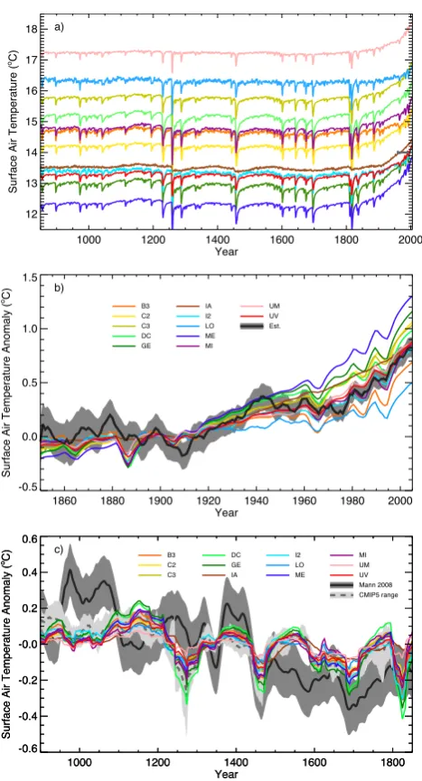
There is a very large range in the absolute SAT simulated over the historical period by the models involved in this in-tercomparison. Absolute SAT is a difficult quantity to mea-sure, but Jones et al. (1999) estimate the absolute global av-erage value of SAT to be approximately 14◦C between the years 1960 and 1990. As seen in Fig. 2a, the annual average SAT at 850 varies from 12.3 to 17.2◦C. All of the models are using similar externally specified forcing, so this large range in initial conditions must be due to internal model differences. Most comparisons between models and obser-vational datasets only examine anomalies from a particular reference period (as in Fig. 2b). However, the large differ-ences between initial states might influence the models’ re-sponses to changing climate forcing. Some feedbacks, such as the albedo changes from reductions in snow or ice, and hence an individual model’s climate sensitivity (Weaver et al., 2007), would likely depend on the models’ initial state.
Although the average model trend over the 20th century (0.79◦C) is close to the observed trends (0.73◦C) (Morice et al., 2012), there is still considerable spread in model response (0.4 to 1.2◦C). One difficulty in comparing EMICs involves the large variation in complexity between models. The imple-mentation of some of the forcing needs to be highly parame-terized or even specified in many models. Aerosols and land-use change can be particularly challenging to implement. A few EMICs are not able to apply all of the forcings specified in the experimental design, which adds to the model spread.
For the specified external forcings over the 20th century, five models appear to stay mostly within the observational uncertainty envelope for this period, five tend to overestimate the observed trends, and two tend to underestimate the trends (Fig. 2b). The model with the largest trend (ME) did not in-clude any sulphate aerosol forcing. Without the cooling as-sociated with this forcing, the model would be expected to overestimate 20th century warming. On the other hand, the UM model, which simulates the 20th century trend well, in-cludes estimates of the indirect effect of sulphate aerosols but not the countering ozone and black carbon forcing (see Appendix B). Given the large number of models included in this intercomparison, the variation in the application of exter-nal forcing appears to average out, and the model mean trend agrees well with observations.
1000 1200 1400 1600 1800 2000 Year
12 13 14 15 16 17 18
Surface Air Temperature (
oC)
a)
1860 1880 1900 1920 1940 1960 1980 2000
Year -0.5
0.0 0.5 1.0 1.5
Surface Air Temperature Anomaly (
oC)
B3 C2 C3 DC GE
IA I2 LO ME MI
UM UV Est.
b)
1000 1200 1400 1600 1800
Year -0.6
-0.4 -0.2 -0.0 0.2 0.4 0.6
Surface Air Temperature Anomaly (
oC)
B3 C2 C3
DC GE IA
I2 LO ME
MI UM UV Mann 2008 CMIP5 range
c)
1000 1200 1400 1600 1800
Year -0.6
-0.4 -0.2 -0.0 0.2 0.4 0.6
Surface Air Temperature Anomaly (
oC)
Fig. 2. Global surface air temperature from the historical all-forcing
simulation for 12 of the participating models. Absolute tempera-tures are shown for the entire simulation in (a). The small dark grey bar at 14◦C between 1960 and 1990 is an estimate of the average absolute surface air temperature from Jones et al. (1999) over this period. Temperature anomalies from 1850 are shown in (b). The dark grey line shows changes in SAT, and the grey shading indi-cates the uncertainty, from Morice et al. (2012). The model results and the data estimates are shown as anomalies from the average over the decade centred at year 1900 and have been processed with a 5 yr moving average, rectangular filter. Temperature anomalies before 1850 are shown in (c). The dark grey line shows changes in global SAT, and the grey shading indicates the uncertainty, from the error-in-variables (EIV) reconstruction of Mann et al. (2008). The grey dashed line shows the model mean, and the light grey shading the model range, of the CMIP5 models that carried out the PMIP3 “last millennium” experiment. The model results and the data estimates are shown as anomalies from the average over the entire period (900 to 1850 or 900 to 1800 for the CMIP5 models) and have been pro-cessed with a 30 yr moving average, rectangular filter.
Given that many factors other than initial state influence a model’s 20th century climate response, a strong relationship is not expected.
Over the pre-industrial period (Fig. 2c), the models tend to show a relatively weak response compared to the Mann et al. (2008) global SAT reconstruction. The reconstruction in-dicates a relatively warm period near year 1000 (often called the Medieval Climate Anomaly, or MCA) and a cooler pe-riod near year 1700 (often referred to as the Little Ice Age, or LIA). In terms of anomalies from today, it is mostly the MCA that is not well reproduced by the models since they agree reasonably well with the reconstructed difference in temperature between the LIA and present climate (∼1◦C).
It does appear that, on average, the models show a stronger cooling response to several large volcanic eruptions than is indicated by the reconstructions (see eruptions near years 1280 and 1810 in Fig. 2). Given that volcanic forcing is gen-erally short-lived, it is difficult to determine if the strong cooling response is due to excessive volcanic forcing or a lack of temporal resolution in the SAT reconstruction. It is also possible some of the proxies used in the reconstructions are not very sensitive to volcanic cooling (Mann et al., 2012). Temperature reconstructions over the last millennium (as in Mann et al., 2008 or Frank et al., 2010) tend to show little agreement.
Several CMIP5 models have also carried out the PMIP3 “last millennium” or CMIP5 “past1000” experiment (bcc-csm1-1, CCSM4, FGOALS-gl, GISS-E2-R, IPSL-CM5A-LR, MIROC-ESM, MPI-ESM-P), and these results are avail-able through the CMIP5 data portal. The range and mean of these CMIP5 model simulations are also shown in Fig. 2c. The mean response of the CMIP5 models is very similar to the mean EMIC response, including a strong SAT response to volcanic forcing. This is perhaps expected since both sets of models are following the same PMIP3 external forcing pro-tocol. A similar strong response to volcanic forcing is also seen in Fern´andez-Donado et al. (2012). Given the low lev-els of internal variability in EMICs, the range in the EMIC’s SAT response is mostly contained within the CMIP5 model range. This weakly forced response between the MCA and LIA, found here in both EMICs and CMIP5 models, is also seen in several other modelling studies – especially for mod-els that specify weak solar irradiance variation between these periods (Goosse et al., 2010; Jungclaus et al., 2010; Servon-nat et al., 2010; Fern´andez-Donado et al., 2012). However, Feulner (2011) finds good agreement with Northern Hemi-sphere temperature reconstructions for a solar constant of 1361 W m−2, weak solar variations and the Crowley (2000) volcanic forcing.
1900 1920 1940 1960 1980 2000 Year
-60 -40 -20 0 20 40
Ocean Heat Content Anomaly (10
22J) B3
C2 C3 DC GE LO
ME MI UV Est. a)
1900 1920 1940 1960 1980 2000 Year
-6 -4 -2 0 2 4
Thermosteric Sea Level Anomaly (cm)
B3 C2 C3 DC GE I2
LO ME MI UV Est. b)
1900 1920 1940 1960 1980 2000 Year
-15 -10 -5 0 5
Change in Atlantic Overturning Index (%)
B3 C2 C3 GE
LO ME MI UV c)
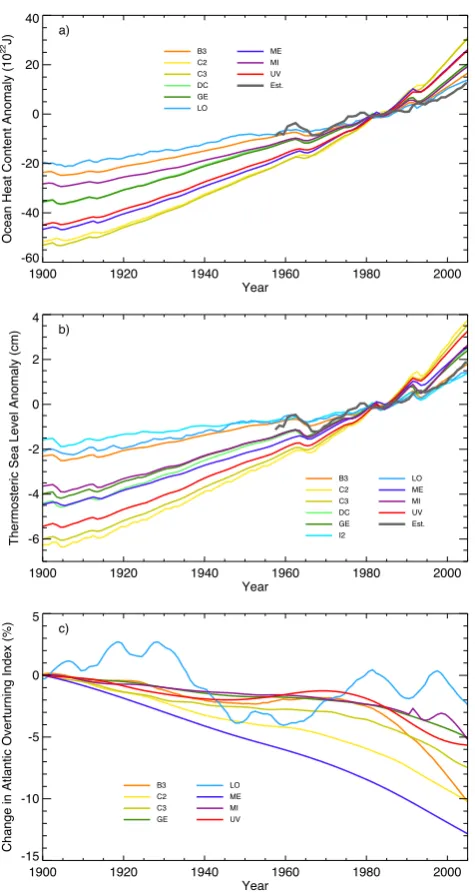
Fig. 3. Changes in global ocean heat content (a), thermosteric sea
level rise (b), and North Atlantic overturning index (c) over the last century. The dark grey lines are estimates of the change in heat con-tent (a), and the thermosteric component of sea level change (b), of the first 2000 m of the ocean, from Levitus et al. (2012). Ocean heat content (a) and thermosteric sea level (b) are plotted as anomalies from the year 1957 to 2005 average. Note that the model heat con-tent and sea level changes are averages over the entire ocean so these would be expected to be somewhat larger than the values estimated over the first 2000 m. The North Atlantic overturning index (c) is shown as a percent change from the decade centred at year 1900 and was processed with a 30 yr moving average, rectangular filter.
that many models may be overestimating ocean heat uptake. Some of the modelled differences from observations could be due to too much or too little surface warming. The two models that agree well with ocean heat uptake estimates are the same models that slightly underestimate atmospheric sur-face warming over the 20th century. Estimates of past ther-mosteric sea level rise (Fig. 3b) show similar differences be-tween the models’ and data estimates, with the models gen-erally simulating more thermosteric sea level rise than ob-served. This is not surprising since the largest component of thermosteric sea level changes is from changes in ocean heat content.
The response of the thermohaline circulation in the At-lantic, as indicated by a simple Atlantic meridional overturn-ing index (defined as the maximum value of the overturnoverturn-ing stream function in the North Atlantic), indicates a moderate slowing in all models (between about 0.8 and 2.1 Sv, or from 3 to 13 %). Direct measurements of the thermohaline circu-lation are difficult, and trends are hard to distinguish from natural variability. There is, therefore, still some controversy as to the response of the meridional overturning circulation over the 20th century (Latif et al., 2006). However, this mod-erate response to a warming climate is similar to what has been seen in previous studies (Plattner et al., 2008).
3.2 Idealized climate response metrics
In order to assess the models’ responses in a more con-trolled environment, several standard idealized experiments were performed. Idealized experiments with CO2increasing
at a rate of 1 % per year until reaching two or four times the initial level of pre-industrial CO2were used to assess the
transient climate response and equilibrium climate sensitiv-ities. Here we define the equilibrium climate sensitivity to be the change in SAT after 1000 yr, even though the mod-els are not truly in equilibrium. There is a relatively large range in the equilibrium climate sensitivity (see Fig. 4a and Table 2). Equilibrium climate sensitivity at 2×CO2ranges
between 1.9 and 4.0◦C, and at 4×CO2 between 3.5 and
8.0◦C. For comparison, the range of 2×CO2 equilibrium
climate sensitivity for CMIP3 models is 2.1 to 4.4◦C, and the range for CMIP5 models is estimated to be 2.1 to 4.7◦C (Andrews et al., 2012). The ocean heat uptake efficiency was also calculated from this 4×CO2idealized experiment, and
it is interesting to note that the model with the highest up-take efficiency (LO) is also one of the models with the low-est ocean heat uptake over the 20th century. This implies that the lower than average (but closer to observed) heat uptake is most likely due to the model’s lower than average 20th cen-tury warming. This may not be the case with B3, which also has lower than average 20th century ocean heat uptake, but shows one of the lowest heat uptake efficiencies.
0 200 400 600 800 1000 Year
0 2 4 6 8
Surface Air Temperature Anomaly (
oC)
B3 C2 C3
DC FA GE
I2 LO ME
MI ML SP
UM UV
a)
-50 0 50
Latitude 0.0
0.5 1.0 1.5 2.0 2.5 3.0
Zonal Temperature Amplification
B3 C2 C3 DC FA
GE IA I2 LO ME
MI ML SP UM UV
b)
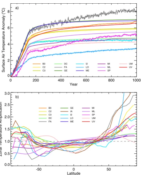
Fig. 4. Surface air temperature (a) and zonal temperature
ampli-fication (b) for all 15 participating models, from a 1 % increase to 4×CO2 simulation. The zonal temperature amplification is calculated as the zonal anomaly divided by the global average anomaly at year 140, which roughly corresponds to the time of CO2 quadrupling.
4×CO2experiment. The temperature amplification at year
70 (when 2×CO2 is reached, not shown) is similar. Some
models (DC, ME, MI, ML) exhibit very little polar amplifi-cation, showing a nearly flat zonal response. Two models (IA and LO) show polar amplification in the north to be larger than 3.0. Although the model with the highest polar amplifi-cation has one of the lowest climate sensitivities, and starts from one of the warmest initial states, there appears to be no simple relationship between polar amplification, climate sensitivity and initial state.
3.3 Historical carbon-cycle response
The ability to reproduce trends in the carbon cycle is another important requirement for models that are used to predict the fate of anthropogenic carbon. For the historical all-forcing experiment (as for RCPs), CO2concentrations are specified,
but models with a complete carbon cycle can still calculate emissions that are compatible with the specified CO2. The
overall average EMIC carbon cycle response for the 1990s is within the uncertainty range of estimated values, except for diagnosed emissions, which are slightly underestimated (see Table 3). The EMIC mean in Table 3 excludes the two models
(ME, UM) that do not transfer carbon with land-use change. These models would be expected to overestimate diagnosed emissions due to the lack of emissions from land-use change. This can be seen in the accumulated fluxes from 1800–2000, where they underestimate land fluxes to the atmosphere, and thus overestimate total diagnosed emissions by 61 to 103 Pg of carbon.
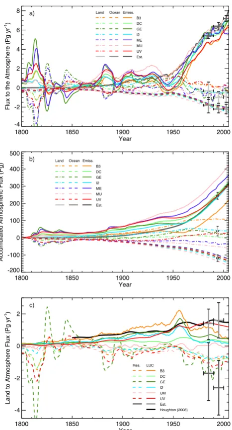
The fluxes of carbon to the atmosphere are shown in Fig. 5a. All models reproduce the estimated fluxes to the ocean within the uncertainty ranges, between 1980 and 2005. Although all models remain within the large range of uncer-tainty for land fluxes in the 1980s, many appear to underesti-mate recent land fluxes, especially since 2000. A few models are able to reproduce trends in emissions reasonably well, but most underestimate recent emissions, apparently because of insufficient net uptake on land.
Figure 5b shows the accumulated fluxes of carbon since 1800. The integral changes in pools (or emissions) are also shown with associated uncertainty as cross bars at 1994 (es-timates from Sabine et al., 2004). Again, all models estimate total ocean uptake within the range of uncertainty (see Ta-ble 3). Total land pool changes are much more variaTa-ble, with only half of the models estimating fluxes within the range of uncertainty. However, most models do remarkably well at estimating total emissions between 1800 and 1994. Two models overestimate total emissions, and one underestimates emissions.
Figure 5c breaks down the land fluxes into two compo-nents. The land-use change (LUC) flux component is esti-mated from a simulation with only land-use change forcing. The residual flux is the total flux from an all-forcing simula-tion minus the LUC component. As in Houghton (2008), the LUC component should not include any interaction between land-use change and changes in climate or CO2. Any
inter-action terms are part of the residual flux. As expected, the UM model, which does not directly include carbon transfer as part of the model’s land-use forcing, shows near-zero LUC carbon fluxes. If the diagnosed LUC flux is correct, then most other models also appear to underestimate carbon fluxes to the atmosphere from LUC. Most models also tend to under-estimate residual land uptake.
It would appear that any underestimation of LUC and the residual flux partially cancel, allowing some models to gener-ate reasonable overall land fluxes. If LUC fluxes were higher, then the residual uptake by land would need to be greater. In general, it would appear that all models are either over-estimating the response of the land carbon cycle to climate change or not taking up sufficient carbon through fertilization of vegetation (either from CO2or deposition of N). Only the
1800 1850 1900 1950 2000 Year
-4 -2 0 2 4 6 8
Flux to the Atmosphere (Pg yr
-1)
Est. UV MU ME I2 GE DC B3 Emiss. Ocean Land
a)
1800 1850 1900 1950 2000
Year -200
-100 0 100 200 300 400 500
Accumulated Atmospheric Flux (Pg)
Est. UV MU ME I2 GE DC B3 Emiss. Ocean Land
b)
1800 1850 1900 1950 2000
Year -4
-2 0 2
Land to Atmosphere Flux (Pg yr
-1)
Houghton (2008) Est. UV UM I2 GE DC B3
Res. LUC
c)
Fig. 5. Carbon fluxes to the atmosphere from the land, ocean and
an-thropogenic emissions since 1800 from models with land and ocean carbon cycle components. Fluxes are shown in (a), the accumulated flux or change in pool carbon in (b) and the components of the land flux in (c). The land-use change (LUC) component was cal-culated from a simulation that only included land-use change forc-ing. The residual component (Res.) is calculated as the difference in land fluxes between a simulation with all forcing and one with just land-use change forcing. The model results in (a) and (c) have been processed with a 10 yr moving average, rectangular filter. The data and uncertainty estimates for the years 1980–1989, 1990–1999 and 2000–2005 in (a) and (c) are from Table 1 in Denman et al. (2007). The data and uncertainty estimates at year 1994 in (b) are from Sabine et al. (2004). The solid black line in (b) indicates fossil fuel emission estimates from Boden et al. (2012) and in (c) the LUC flux estimates from Houghton (2008).
current response does not appear to be well simulated by most models.
It is possible that the diagnosed partitioning between the LUC and residual flux is poorly estimated by the LUC only forcing simulation – at least in terms of the definition of Houghton (2008). There may be a small feedback on the car-bon cycle due to the cooling from local albedo changes. Ad-ditional simulations with GENIE (not shown) indicate that there is likely some underestimation of LUC fluxes in the simulation with only land-use forcing due to the climate– carbon feedback on soil respiration. The cooling from the albedo change reduces soil respiration, which in turn reduces the apparent LUC flux. Simulations with fixed albedo (and thus climate) indicate that this underestimation may be sig-nificant. Further investigation is required to determine if this small feedback leads to a significant underestimation of the LUC flux in other models.
3.4 Idealized carbon-cycle response metrics
Standard carbon cycle metrics are also calculated from spec-ified 1 % increasing to 4×CO2experiments. In addition to
the standard fully coupled experiment, two additional par-tially coupled experiments were done by EMICs with a com-plete carbon cycle. One experiment excluded only the direct greenhouse radiative effects of increasing CO2 (radiatively
uncoupled) while the other experiment excluded only the direct effects of increasing CO2 on land and ocean carbon
fluxes (biogeochemically uncoupled). For specified CO2
ex-periments, the CO2concentration–carbon sensitivity (β) can
be calculated directly as the change in land or ocean carbon divided by the change in atmospheric CO2 in a radiatively
uncoupled simulation. The climate–carbon sensitivity (γ) is calculated directly as the change in land or ocean carbon di-vided by the change in SAT in a biogeochemically uncoupled simulation.
These parameters are calculated differently from the C4MIP intercomparison project (Friedlingstein et al., 2006) due to the specification of CO2 concentrations rather than
emissions, which results in somewhat lower estimates ofγ
(Plattner et al., 2008; Gregory et al., 2009; Zickfeld et al., 2011). Carbon cycle sensitivities can also be calculated indi-rectly from the difference between a fully coupled simulation and either a biogeochemically uncoupled simulation (forγ) or a radiatively uncoupled simulation (forβ). The value ofγ, and to a lesser extentβ, is highly dependent on the method of calculation for models with large nonlinear climate and CO2interactions (Zickfeld et al., 2011). Plattner et al. (2008)
calculatedβdirectly andγ indirectly.
Directly calculated sensitivities at year 140 (and year 995) are shown in Table 4, and Fig. 6 shows how these sensitivities change through time. The CO2concentration–carbon
sensi-tivities for land (βL) are relatively constant after 140 yr (CO2
quadrupling) for most models. This is similar forγL, except
Table 2. Standard metrics that help characterize model response.TPI is the average surface air temperature between 850 and 1750, and
1T20this the change in surface air temperature over the 20th century, both from the historical “all” forcing experiment. TCR2X, TCR4X, and ECS4Xare the changes in global average model surface air temperature from the decades centred at years 70, 140, and 995 respectively, from the idealized 1 % increase to 4×CO2experiment. The ocean heat uptake efficiency,κ4X, is calculated from the global average heat flux divided by TCR4Xfor the decade centred at year 140, from the same idealized experiment. Note that ECS2xwas calculated from the decade centred at about year 995 from a 2×CO2pulse experiment.
Model TPI 1T20th TCR2X ECS2x TCR4X ECS4X κ4X (◦C) (◦C) (◦C) (◦C) (◦C) (◦C) (W m−2C−1)
B3 14.6 0.57 2.0 3.3 4.6 6.8 0.58
C2 14.2 0.91 2.1 3.0 4.7 5.8 0.84
C3 15.7 0.91 1.9 3.2 4.5 5.9 0.93
DC 15.1 0.84 2.1 2.8 3.9 4.8 0.72
FA – – 2.3 3.5 5.2 8.0 0.55
GE 12.9 1.00 2.5 4.0 5.4 7.0 0.51
IA 13.5 0.80 1.6 – 3.7 4.3 –
I2 13.3 0.70 1.5 1.9 3.7 4.5 –
LO 16.3 0.38 1.2 2.0 2.1 3.5 1.17
ME 12.3 1.15 2.4 3.7 5.3 6.9 0.55
MI 14.7 0.71 1.6 2.4 3.6 4.6 0.66
ML – – 1.6 2.8 3.7 5.5 1.00
SP – – 0.8 3.6 2.9 5.2 0.84
UM 17.2 0.79 1.6 2.2 3.2 4.3 –
UV 13.2 0.75 1.9 3.5 4.3 6.6 0.92
EMIC mean 14.8 0.78 1.8 3.0 4.0 5.6 0.8 EMIC range 12.3 to17.5 0.38 to 1.15 0.8 to 2.5 1.9 to 4.0 2.1 to 5.4 3.5 to 8.0 0.5 to 1.2
Table 3. Average carbon fluxes to the atmosphere over the 1990s and accumulated carbon fluxes from 1800 to 1994. LandLUCis an estimate
of land-use change fluxes from simulations with only land-use forcing. LandResis the residual land flux, which is derived from the land flux from a simulation with all forcing minus LandLUC. All other model fluxes are from differences between the all-forcing and control simulations. Estimates of average fluxes are from Table 7.1 of Denman et al. (2007), and estimates of accumulated fluxes are from Table 1 of Sabine et al. (2004). The change in atmospheric carbon storage between 1800 and 1994 is estimated to be 164±4 Pg in Sabine et al. (2004). Although the change in CO2between 1800 and 1994 was specified to be 75 ppm in the all-forcing simulations, due to different estimates of atmospheric volume, the change in atmospheric carbon storage in the models is between 158 and 165 Pg.
Average carbon flux: 1990 to 1999 (Pg yr−1) Accumulated flux: 1800 to 1994 (Pg) Model LandLUC LandRes Ocean Emissions Land Ocean Emissions
B3 0.7 −0.8 −1.8 5.2 108 −104 167
DC 0.3 −0.9 −1.8 5.7 4 −102 260
GE 0.5 −1.4 −2.1 6.1 21 −114 251
I2 0.3 −0.7 −2.2 5.9 43 −122 237
ME∗ −0.6 −1.9 5.9 −38 −102 305
UM∗ −0.6 −2.4 6.2 −51 −136 344
UV 1.3 −1.2 −2.0 5.2 24 −112 251
EMIC mean∗ 0.6 −1.0 −2.0 5.6 40 −111 233 EMIC range∗ 0.3 to 1.3 −1.4 to−0.7 −2.2 to−1.8 5.2 to 6.1 4 to 108 −122 to−102 167 to 260 Estimates 1.6 −2.6 −2.2 6.4 39 −118 244 Uncertainty 0.5 to 2.7 −4.3 to−0.9 −2.6 to−1.8 6.0 to 6.8 11 to 67 −137 to−99 224 to 264
∗The ME and UM models were excluded from the EMIC model mean and range calculations, because they did not include any direct carbon exchange due to
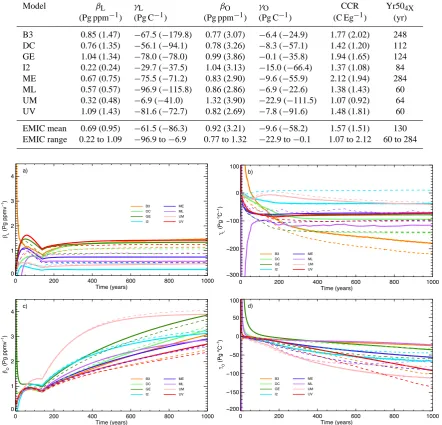
Table 4. Carbon cycle sensitivities and metrics from idealized 4 ×CO2experiments.βL(orβO) is the change in land (or ocean) carbon divided by the change in atmospheric CO2in a radiatively uncoupled simulation.γL(orγO) is the change in land (or ocean) carbon divided by the change in atmospheric temperature, in a biogeochemically uncoupled simulation. CCR is the carbon-climate response and is calculated as atmospheric temperature change divided by diagnosed emissions (Matthews et al., 2009).βL,γL,βO,γO, and CCR are all averages over the decade centred at about year 140 from a 1 % increase to 4×CO2experiment. Numbers in parentheses are averages over the decade centred at year 995. Yr504Xis the year that emissions remaining in the atmosphere fall below 50 %, from an instantaneous 4×CO2pulse experiment.
Model βL γL βO γO CCR Yr504X
(Pg ppm−1) (Pg C−1) (Pg ppm−1) (Pg C−1) (C Eg−1) (yr) B3 0.85 (1.47) −67.5 (−179.8) 0.77 (3.07) −6.4 (−24.9) 1.77 (2.02) 248 DC 0.76 (1.35) −56.1 (−94.1) 0.78 (3.26) −8.3 (−57.1) 1.42 (1.20) 112 GE 1.04 (1.34) −78.0 (−78.0) 0.99 (3.86) −0.1 (−35.8) 1.94 (1.65) 124 I2 0.22 (0.24) −29.7 (−37.5) 1.04 (3.13) −15.0 (−66.4) 1.37 (1.08) 84 ME 0.67 (0.75) −75.5 (−71.2) 0.83 (2.90) −9.6 (−55.9) 2.12 (1.94) 284 ML 0.57 (0.57) −96.9 (−115.8) 0.86 (2.86) −6.9 (−22.6) 1.38 (1.43) 60 UM 0.32 (0.48) −6.9 (−41.0) 1.32 (3.90) −22.9 (−111.5) 1.07 (0.92) 64 UV 1.09 (1.43) −81.6 (−72.7) 0.82 (2.69) −7.8 (−91.6) 1.48 (1.81) 60 EMIC mean 0.69 (0.95) −61.5 (−86.3) 0.92 (3.21) −9.6 (−58.2) 1.57 (1.51) 130 EMIC range 0.22 to 1.09 −96.9 to−6.9 0.77 to 1.32 −22.9 to−0.1 1.07 to 2.12 60 to 284
0 200 400 600 800 1000
Time (years) 0
1 2 3 4
βL
(Pg ppmv
−1) B3
DC GE I2
ME ML UM UV a)
0 200 400 600 800 1000
Time (years) −300
−200 −100 0 100
γL
(Pg
oC
−1
)
B3 DC GE I2
ME ML UM UV b)
0 200 400 600 800 1000
Time (years) 0
1 2 3 4
βO
(Pg ppmv
−1)
B3 DC GE I2
ME ML UM UV c)
0 200 400 600 800 1000
Time (years) −200
−150 −100 −50 0 50 100
γO
(Pg
oC
−1
)
B3 DC GE I2
ME ML UM UV d)
Fig. 6. Land and ocean carbon cycle sensitivities, diagnosed from a 1 % increase to 4×CO2experiment, for models with land and ocean
carbon cycle components. The CO2concentration–carbon sensitivity for land (βL) is shown in (a) and for ocean (βO) in (c). The climate– carbon sensitivity for land (γL) is shown in (b) and for ocean (γO) in (d). The solid lines indicate sensitivities calculated directly from partially coupled experiments while the dashed lines indicate sensitivities calculated indirectly as differences between partially and fully coupled experiments. See the main text for details.
large continuing change inγL in the B3 model is likely due
to the inclusion of permafrost in that model, which reacts to climate change over much longer timescales than most other land processes. The I2 model has the lowest value of
βL, and this is likely due to nitrogen limitation reducing land
uptake in this model (Sokolov et al., 2008). Over the ocean,
the changes in both sensitivities, βO andγO, largely occur
after year 140 (CO2quadrupling). As expected, the response
The dashed lines in Fig. 6 show sensitivities calculated in-directly (as differences from fully coupled simulations). If
γLis calculated indirectly, the I2 model indicates a positive
rather than a negative land sensitivity (see Fig. 6b). This is due to a strong interaction between climate warming, which causes an increase in nitrogen availability and photosynthe-sis, and land carbon uptake. When calculated indirectly, the interaction is strong enough to change the climate–carbon feedback on atmospheric CO2from positive to negative for
the I2 model. UM also has a positiveγL for a short period
when calculated indirectly, while all other models always show negativeγL, using either method of calculation. UV,
B3, GE and ME always show more negativeγ andβ, while I2 and UM always show more positiveγ andβ, when these sensitivities are calculated indirectly rather than directly. ML shows more positive sensitivities for land and more nega-tive for the ocean, while DC is the opposite, when γ and
β are calculated indirectly rather than directly. Presumably the nonlinear interactions that cause bothγ andβto always change in the same direction (depending on the calculation method, for either the ocean or land) must be very different in the models.
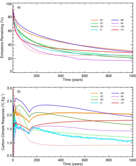
Figure 7a shows the residence time of CO2emissions from
a 4×CO2pulse simulation. This pulse is equivalent to about
1800 Pg. As seen in Table 4, the EMIC mean time for half of the emitted CO2 to be absorbed by the land and ocean
sinks is 130 yr. This is considerably longer than the estimate of 30 yr to remove 50 % of emissions given in Chapter 7 of the AR4 (Denman et al., 2007). The main reason for this dif-ference is that the emission pulses used to assess the CO2
absorption timescales in the AR4 were small (40 Pg) com-pared to both the pulse used here and any likely future sions. Absorption timescales depend on the amount of emis-sions (Maier-Reimer and Hasselmann, 1987; Archer et al., 2009; Joos et al., 2012), and this could have been stated more clearly in Chapter 7 of the AR4. Two models (B3 and ME) show considerably longer times to absorb half of emissions. The longer time for the B3 model is likely due to the in-creasing climate feedback over land due to the inclusion of permafrost and peat in that model.
The carbon-climate response has been proposed as a sim-ple metric that combines both the climate and carbon cy-cle sensitivities into a single value. It has been suggested that this metric is relatively insensitive to emission scenar-ios and is approximately constant over several hundred years (Matthews et al., 2009). Figure 7b shows the CCR from a 1 % increasing CO2 experiment which has zero emissions after
reaching 4×CO2. The EMIC results show that, at least for
this scenario, CCR is not constant over time for any of the models, although the intra-model range is smaller for most models than the inter-model range. This metric decreases in all models until emissions are set to zero. After CO2is
al-lowed to freely evolve, CCR generally increases and then declines in most models. After emissions are set to zero, any changes in CCR are just due to changes in SAT and so
0 200 400 600 800 1000
Time (years) 0.5
1.0 1.5 2.0 2.5 3.0
Carbon-Climate Response (
oC Eg -1)
B3 DC GE I2
ME ML UM UV b)
200 400 600 800 1000
Time (years) 0
20 40 60 80 100
Emissions Remaining (%)
B3 DC GE I2
ME ML UM UV a)
Fig. 7. Indicators of climate change longevity. The percentage of
emissions remaining from a 4×CO2 pulse experiment is shown in (a), and the carbon-climate response (CCR) from a 1 % increase to 4×CO2experiment is shown in (b). CO2is allowed to freely evolve in both experiments once CO2has reached 4 times the initial preindustrial level. This is equivalent to about 1800 Pg of carbon emissions. CCR is calculated as the change in SAT divided by the accumulated, diagnosed emissions. After year 140, emissions are zero and any changes in CCR are just due to changes in temperature.
CCR becomes a measure of a model’s zero emissions com-mitment. Two models show a continual increase while one shows a continual decrease. At the time of CO2doubling, the
range in CCR is between 1.4 and 2.5◦C Eg−1of carbon (1 Eg or Tt = 1000 Pg or Gt), and after 500 yr the range is between 0.9 and 2.3◦C Eg−1. Further discussion of the response of CCR in these models can be found in Zickfeld et al. (2013).
3.5 Contributions of forcing components to
temperature
Several experiments were designed to examine the linear-ity of temperature and carbon cycle response to various climate forcings. In each experiment, only one major cli-mate forcing was allowed to vary over the historical period (years 850 to 2005). The individual experiments applied forc-ing from “additional” or non-CO2greenhouse gases (AGG),
CO2 (CO2), land-use change (LUC), orbital (ORB), solar
the individual forcing experiments compared to the experi-ment that applied all forcings together. Since specified CO2
forcing is treated separately, any changes in CO2due to other
forcings, either directly, as with land-use change, or indi-rectly, through climate–carbon feedbacks, are included as part of the CO2forcing.
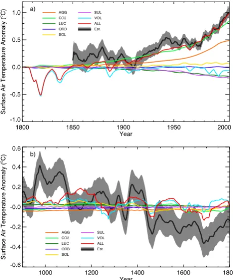
As expected, most of the change in SAT over the last mil-lennium has occurred after industrialization (Fig. 8a). Since 1800, the direct albedo effect from land-use change caused a model average cooling of roughly 0.2◦C, while sulphate forcing also caused a cooling of about 0.2◦C. The sulphate forcing may seem weak, but it is mostly due to the exclu-sion of the indirect forcing from sulphates in the experimen-tal design. The lack of negative forcing from the indirect ef-fect of sulphates is balanced by also excluding similar posi-tive forcing from ozone and black carbon (see Appendix B). The change in solar luminosity since 1800 was found to have a small positive effect on SAT (<0.1◦C). Non-CO
2
green-house gases have had a large influence on SAT since 1800, but this is largely countered by the combined negative forc-ing from land use and aerosols. As a result, CO2 alone is
capable of providing the vast majority of the climate change signal since pre-industrial times.
Before industrialization, the net changes in SAT from any of the forcings over the previous 1000 yr are much weaker, although there are warmer and cooler periods during that time (Fig. 8b). It appears that changes in solar forcing have the largest effect on SAT over long timescales in these sim-ulations. Over the last millennium, orbital forcing was found to have almost no effect on modelled SAT, at the hemispheric scale, in the annual mean, while LUC is associated with a small long-term cooling. Volcanic aerosol forcing has a large but short-lived negative effect on modelled SAT. This agrees with the conclusions of Shindell et al. (2003) and Fern´andez-Donado et al. (2012), although Schneider et al. (2009), Feulner (2011), Miller et al. (2012), and Schleussner and Feulner (2012) indicate the possibility of large volcanic forc-ing causforc-ing longer term persistent coolforc-ing in polar regions. Volcanic forcing does, however, contribute to the cooling be-tween the MCA and the LIA because of the larger number of big eruptions during the latter period (see also Fig. 11).
As noted earlier, the models appear to underestimate the SAT changes between the MCA and the LIA com-pared to reconstructions (Mann et al., 2008; Frank et al., 2010). With similar forcing, the CMIP5 models also show a similar small change in SAT simulated over this period (Fig. 1c). A relatively small change in simulated SAT be-tween the MCA and LIA is also seen in Fig. 15 of Goosse et al. (2010). The low solar variation simulations (E1) of Jungclaus et al. (2010) similarly show small longer term (>100 yr) changes in SAT between the MCA and LIA (see their Fig. 3), although shorter term variability can produce larger differences. Fern´andez-Donado et al. (2012) show that models (EC5MP-E1 and CSIRO; see their Fig. 1) with low, long-term solar variability (labelled ssTSI and similar to the
1800 1850 1900 1950 2000
Year -1.0
-0.5 0.0 0.5 1.0
Surface Air Temperature Anomaly (
oC)
AGG CO2 LUC ORB SOL
SUL VOL ALL Est.
a)
1000 1200 1400 1600 1800
Year -0.6
-0.4 -0.2 -0.0 0.2 0.4 0.6
Surface Air Temperature Anomaly (
oC)
AGG CO2 LUC ORB SOL
SUL VOL ALL Est.
b)
Fig. 8. Individual forcing component contributions to the total
global surface air temperature response. The model results are from the average of 11 models: B3, C2, C3, DC, GE, I2, LO, MI, ME, UM and UV. The response after 1800 is shown in (a). The dark grey line shows changes in global SAT, and the grey shading indicates the uncertainty, from Morice et al. (2012). The model results and the data estimates were processed with a 5 yr moving average, rectan-gular filter. Model results are shown as anomalies from the decade centred at 1800. The data estimates are shown as an anomaly, which has been offset to show the same SAT anomaly as the all-forcing av-erage over the decade centred on the year 1900. The response before 1800 is shown in (b). The dark grey line shows changes in global SAT, and the grey shading indicates the uncertainty, from the EIV reconstruction of Mann et al. (2008). Model results and data esti-mates are shown as anomalies from their average over the entire period (850 to 1850) and have been processed with a 30 yr moving average, rectangular filter.
Schmidt et al. (2012) solar forcing used here) simulate very small SAT changes between the MCA and LIA (∼0.1◦C; see their Fig. 6).
3.6 Linearity of the forced response
Figure 9a shows the difference between the anomalous re-sponse of the all-forcing experiment and the sum of the anomalous responses of the individual forcing simulations. If the climate system responded linearly to the individual forc-ings, then the resulting summation would be zero. In gen-eral this is the case for all models. There are some ences after 1900 for the ME and UM model, but these differ-ences are still small compared to overall noise. It may be that EMICs are too simple to demonstrate significant nonlineari-ties, but given the diversity in the complexity of EMICs, this seems unlikely. Fern´andez-Donado et al. (2012) also sug-gest a high degree of linearity between forcing and simulated temperature.
Figure 9b shows similar results for diagnosed carbon emis-sions. Here some models appear to show an interaction be-tween individual forcing that is larger than noise, particularly the UV model. This interaction is between land-use change and CO2 forcing. In models that simulate land-use forcing
by removing vegetation (B3, GE, I2 and UV), it would be expected that there would be less CO2fertilization due to the
removal of vegetation from land-use change (Strassmann et al., 2008). This reduction in land uptake by CO2fertilization
would result in lower diagnosed emissions and thus total car-bon in a simulation that has both land-use change and CO2
fertilization acting together. In the DC model most of the land carbon removed by land-use change was taken from the soil rather than from the vegetation and so this model would not be expected to show a strong interaction. The ME and UM models also do not show this interaction between vegetation removal (due to land-use change) and the CO2fertilization
feedback since they do not reduce vegetation or directly ex-change carbon with land use. The UV model has one of the largest CO2concentration–carbon sensitivities (Table 4) and
the largest recent land-use emissions (Table 3). As such, it shows the largest interaction between land-use change and CO2. The GE model is not shown, because one of the
en-semble members that constitute the enen-semble mean was not useable.
3.7 Changes in climate from natural and
anthropogenic forcing
Freely evolving CO2simulations have the advantage of not
forcing the model into a specified state. Thus, these types of experiments can show how CO2might change under
differ-ent scenarios. Two historical simulations in which CO2was
allowed to freely evolve were conducted to determine the an-thropogenic influence on the carbon cycle. While one simu-lation applied natural forcing, the other included natural and anthropogenic forcing, including specified emissions from fossil fuel combustion. The anomalous SAT from these two simulations since 1750 is shown in Fig. 10. The range in the simulations with only natural forcing is very small compared
1000 1200 1400 1600 1800 2000
Year -0.2
-0.1 0.0 0.1 0.2 0.3
Surface Air Temperature Difference (
oC)
B3 C2
C3 DC
I2 ME
UM UV a)
1000 1200 1400 1600 1800 2000
Year -40
-30 -20 -10 0 10
Carbon Difference (Pg)
B3 DC I2
ME UM UV b)
Fig. 9. The linearity of the surface air temperature response (a) and
carbon fluxes to the atmosphere (b) over the last millennium. Differ-ences are between anomalies from the all-forcing simulation and the sum of the anomalies from all of the individual forcing component simulations. Model results have been processed with a 5 yr moving average, rectangular filter. The differences are shown as anomalies from the average of the century centred at about year 1000. If the in-dividual component responses added linearly to the total response, then the differences should be zero.
to the range of the models when anthropogenic forcing is also applied. This is not surprising since the magnitude of the an-thropogenic forcing is much greater than the magnitude of the natural forcing, so any differences in model response are amplified. The simulations with only natural forcing produce almost no change in overall SAT between 1750 and 2005. As seen in many other studies (see Hegerl et al., 2007 for a review), when only natural forcing is applied, the models are not capable of simulating the rise in SAT that has been observed over this time period.
1750 1800 1850 1900 1950 2000 Year
-1.5 -1.0 -0.5 0.0 0.5 1.0 1.5
Surface Air Temperature Anomaly (
oC)
Est. UV UM ME I2 GE DC B3
Nat. All
Fig. 10. The surface air temperature response of the models in freely
evolving CO2simulations that include only natural forcing (Nat.) or all-forcing (All). Note all-forcing includes both natural (orbital, so-lar, stratospheric and volcanic aerosols) and anthropogenic (green-house gas, land use, tropospheric aerosol) forcing. As in Fig. 7, the light grey shading indicates the uncertainty range in SAT, from Morice et al. (2012). The model results and the data estimates were processed with a 5 yr moving average, rectangular filter. Model re-sults are shown as anomalies from the decade centred at 1750. The data uncertainty estimates are shown as an anomaly, which has been offset to show the same SAT anomaly as the model average over the decade centred on the year 1900.
and disparate. Models may then be useful in assessing the plausibility of differing palaeoclimate reconstructions, by al-lowing reconstructions and forcing to be compared in a phys-ically consistent manner.
3.8 Changes in temperature between the MCA
and the LIA
The pre-industrial SAT anomalies from the naturally forced, freely evolving CO2simulation are shown in Fig. 11a. The
models simulate a modest MCA and a small decline in SAT into the LIA that is similar to the specified CO2experiment.
Although there is considerable uncertainty, estimates from palaeoclimate reconstructions suggest about 0.38◦C as the difference between the warmest (1071–1100) and coolest (1601–1630) pre-industrial periods in the Northern Hemi-sphere over the last millennium (Frank et al., 2010). The start and end of these climate periods are still debated, but for the simple analysis used here we define an MCA index period to be between 1100 and 1200, and a LIA index pe-riod between 1600 and 1700. The 100 yr pepe-riods used for these indices were chosen to represent the models’ warmest period between year 950 and 1250 and the coolest period be-tween 1450 and 1750. These periods are slightly later than the times estimated from reconstructions for the highest and lowest temperature change for the pre-industrial portion of the last millennium (Frank et al., 2010). Between these 100 yr MCA and LIA periods, the model average difference in glob-ally averaged SAT is 0.19◦C. The largest difference occurs
in GE, which simulates a drop in temperature of 0.33◦C
be-tween the reference periods.
For the all-forcing simulation (with land-use change and specified CO2), the average EMIC global SAT response for
the transition between the MCA and the LIA index periods is about 0.21◦C (see Fig. 11b). The slightly smaller change in SAT in the naturally forced, free CO2simulation is in part
due to the lack of cooling from land-use change (which is not included in the natural forcing simulation), but mostly be-cause the simulated drop in CO2is not as great as suggested
from ice cores (see Fig. 11c). With the additional cooling from the specified reduction in CO2, the largest difference
once more occurs in GE, which simulates a drop in tem-perature of 0.35◦C. It is, however, difficult to compare SAT changes averaged over different periods and regions. For ex-ample, the UV model simulates a 0.05◦C greater drop in SAT
over the Northern Hemisphere (for which the observational estimate was reconstructed) than globally. However, even af-ter correcting for this difference, most models appear to be underestimating the change in SAT over this period.
The lack of cooling in the models may be from underes-timating the specified forcing changes over this period. The individual forcing component contributions to the change in SAT are shown in Fig. 11b. The CO2, solar and volcanic
forcings are, in nearly equal proportions, the major contrib-utors to the total drop in SAT between the MCA and the LIA index periods. There is also a small cooling contribu-tion from the direct climate effects of land-use change, and very small warming contributions from changes in orbit and non-CO2greenhouse gases. There are earlier periods in the
simulations that are as cold or nearly as cold as the LIA in-dex period. These early minima in simulated temperature are mostly caused by a series of volcanic eruptions.
3.9 Changes in CO2between MCA and LIA
CO2can be extracted directly from ice cores and is relatively
well reconstructed over the past millennium, although there are still uncertainties in both the timing of the CO2 record
and in determining how well CO2records from individual ice
cores represent global values. The large fluctuations in mod-elled CO2 before the LIA are not seen in the PMIP3 CO2
dataset (Fig. 11c and d), although other records may be more variable (Mitchell et al., 2011). If we assume that the CO2
record is accurate and that changes in CO2 are determined
by changes in SAT over this period (through climate–carbon cycle feedbacks), then there would appear to be an inconsis-tency between the lack of change in the CO2record and the
large model temperature changes generated by the (mostly volcanic) forcing before the LIA. This implies the follow-ing: the specified volcanic forcing is not realistic, or the CO2
record is not reliable, or the climate–carbon cycle feedback is weak or masked in the CO2record by other factors. It is
1200 1400 1600 Year
-0.4 -0.2 0.0 0.2
Surface Air Temperature Anomaly (
oC)
B3 DC GE I2 ME UM UV Mean
a)
MCA LIA
1200 1400 1600
Year -0.4
-0.2 0.0 0.2
Surface Air Temperature Anomaly (
oC)
AGG CO2 LUC ORB SOL SUL VOL ALL
b)
MCA LIA
1200 1400 1600
Year -10
-8 -6 -4 -2 0 2
CO
2
Anomaly (ppmv)
B3 DC GE I2 ME UM UV Mean Est.
c)
MCA LIA
1200 1400 1600
Year -10
-8 -6 -4 -2 0 2
CO
2
Anomaly (ppmv)
B3 DC GE I2 ME UM UV Mean Est.
d)
MCA LIA
Fig. 11. Comparison of global surface temperature and CO2responses over the preindustrial portion of the last millennium. The surface air
temperature responses in (a) are from the freely evolving CO2simulations with only natural forcing. The contributions of individual forcing components to the temperature response, shown in (b), are model averages from experiments with specified CO2. The model averages in (b) are from 11 models: B3, C2, C3, DC, GE, I2, LO, MI, ME, UM and UV. Maximum Northern Hemisphere SAT changes between the MCA and LIA are estimated to be about 0.4◦C from palaeoclimate reconstructions, but this is highly uncertain (Frank et al., 2010). The CO2 response is shown for the freely evolving CO2simulations with only natural forcing in (c) and all-forcing in (d). When multiple model results are shown, the model mean is indicated by a dashed grey line. The solid dark grey lines in (c) and (d) are an estimate of reconstructed CO2from the PMIP3 forcing dataset (Schmidt et al., 2012). Horizontal lines over two, century-long index periods (1100–1200 and 1600– 1700), which roughly correspond to the Medieval Climate Anomaly (MCA) and Little Ice Age (LIA), indicate model or data averages over these periods. All model results and data estimates are shown as anomalies from the average over the years 1100 to 1200 and were processed with a 30 yr moving average, rectangular filter.
Along with temperature, the models also seem to underes-timate the reduction in CO2during the MCA–LIA transition.
The model average reduction in CO2is 2.4 ppm compared to
7.9 ppm from the PMIP3 protocol reconstruction (Schmidt et al., 2012), calculated over the same MCA and LIA index pe-riods. Since most models appear to have a positive climate– carbon cycle feedback over this period (see Fig. 11a and c), some of the small reduction in CO2would be attributable to
an underestimated reduction in SAT.
3.10 Estimating the carbon-climate sensitivity from the
MCA to LIA transition
Assuming all of the reduction in CO2 is driven by
changes in climate, a crude estimate of the climate feed-back can be calculated from the simulated change in CO2
and SAT over the MCA–LIA transition. This estimate of the climate–carbon cycle sensitivity has a model average of 2.4 ppm/0.19◦C = 12.6 ppm◦C−1, with a range between
5.1 and 18.8 ppm◦C−1. This estimate is relatively
insensi-tive to the reference periods. Using the average change in SAT and CO2between 950 to 1250, and 1450 to 1750 yields
very similar results (model average of 13.5 ppm◦C−1 with a range between 4.5 and 23.3 ppm◦C−1). If this estimate of sensitivity were to hold for larger changes in temperature, then the model average drop in CO2for a 0.4◦C reduction
in temperature would be 5.1 ppm. Even scaling the response of the model with the largest sensitivity (18.8 ppm◦C−1for B3) would still only produce a drop in CO2of 7.5 ppm.
Ap-parently, in order to simulate the large observed drop in CO2
during the MCA–LIA transition, either the temperature drop must be larger than 0.4◦C or the climate–carbon cycle feed-back must be large (>18 ppm◦C−1).
Few models have attempted to simulate a closed car-bon cycle over the past millennium. Gerber et al. (2003) used a carbon cycle model with a sensitivity of about 12 ppm◦C−1 to constrain the temperature transitions over
1◦C. Both Goosse et al. (2010) and Jungclaus et al. (2010)
have used sophisticated models to simulate the evolution of CO2over the past millennium. Goosse et al. (2010) show
al-most no change in CO2betw