Trend Analysis of Temperature Data for Narayani
River Basin, Nepal
Mohan Bahadur Chand1,∗ , Bikas Chandra Bhattarai2 , Prashant Baral3 and Niraj Shankar Pradhananga4
1 Graduate School of Environmental Science, Hokkaido University, Hokkaido 060-0810, Japan;
2 Department of Geosciences, University of Oslo, Blindern 0316 OSLO, Norway; [email protected]
3 Geographic information Systems (GIS) Area, NIIT University, Rajasthan 301705, India; [email protected]
4 Department of Hydrology and Meteorology, Government of Nepal, Kathmandu 44600, Nepal;
* Correspondence: [email protected]
Received: 21 February 2019; Accepted: 1 April 2019;
First Version Published: 3 April 2019 (doi:10.3390/sci1010021)
Abstract: Study of spatiotemporal dynamics of temperature is vital to assess changes in climate, especially in the Himalayan region where livelihoods of billions of people living downstream depends on water coming from the melting of snow and glacier. To this end, temperature trend analysis is carried out in Narayani river basin, a major river basin of Nepal characterized by three climatic regions: tropical, subtropical and alpine. Temperature data from six stations located within the basin are analyzed. The elevation of these stations ranges from 460 to 3800 m asl. and the time period of available temperature data ranges from 1960–2015. Multiple regression and empirical mode decomposition (EMD) methods are applied to fill in the missing data. Annual as well as seasonal trends are analyzed and Mann-Kendall test is employed for testing the statistical significance of detected trend. Results indicate significant cooling trends before 1970s, and warming trends after 1970s in the majority of the stations. The warming trends range from 0.028◦C per year to 0.035 ◦C per year with a mean increasing trend of 0.03◦C per year after 1971. Seasonal trends show
highest warming trends in monsoon season followed by winter, pre-monsoon, and post-monsoon season. However, difference in warming rates between different seasons isn’t sufficiently large. An average temperature lapse rate of−0.006◦C per m with the steepest value (−0.0064◦C per m) in pre-monsoon season and least negative (−0.0052◦C per m) in winter season is observed for this basin. A comparative analysis of the gap-filled data with freely available global climate data sets shows reasonable correlation thus confirming the suitability of the gap filling methods.
Keywords:climate change; temperature trend; Himalaya; river basin; Nepal
1. Introduction
Climate Change and global warming are widely recognized as the most significant dilemma the world is experiencing today [1]. Studies based on direct measurements and remote sensing have suggested that increase in the atmospheric concentration of greenhouse gases are causing the global climate change [2]. Global temperatures are significantly rising since last decade, despite year-to-year fluctuations associated with the El Niño-La Niña cycle of tropical ocean temperature [3]. Linear warming trends from 1951 to 2012 show an increase of global temperature by 0.12◦C per decade [2]. However, the rate of increase of temperature are different for different regions. The widespread retreat of mountain glaciers and snow cover due to increasing temperatures have contributed to sea level
rise [2]. This warming are also expected to have significant impacts on the hydrological cycle of mountain river basins affecting livelihoods of population living downstream.
The Hindu-Kush Himalayan (HKH) region is characterized by mountainous environments [4]. Weather and climatic conditions over the Himalayan regions are of great interest to the scientific community [5]. HKH has the highest elevation range in the world and contains largest freshwater reserve in the form of snow and glacier ice outside the Polar Regions. Several studies have reported warming in the Himalayan region [6] which has caused shrinkage of glaciers [7–9], expansions of glacier-fed lakes [10–12], degradation of permafrost [13] and changes in the hydrological cycle of many mountain rivers [14,15]. For example, Lama et al. [9] reported a loss of about 22% of the glacier area in Mustang, within Narayani basin from 1980s-2010. The temperature is increasing faster than the global average in the Tibetan Plateau and Northern Hemisphere [16], Himalayan region and the influence of rising temperatures is greater in the Eastern Himalayas compared to that in the greater Himalayas [17]. An increasing trend of annual average temperature is observed in Tibetan plateau [4,16], Sutluj River basin, Western Himalayan region [6], Nepal Himalayas [18], Karnali River basin, Nepal [19], southern slope of Nepal Himalayas [20]. Shrestha et al. [18] analyzed the maximum temperature since 1977 and found a warming trend of temperature by 0.06◦C to 0.12◦C per year in Middle Mountain and Himalayan region and by 0.03◦C in Siwalik and southern plains. Kattel and Yao [20] reported an increase in temperature by 0.038◦C per year in mountain stations of Nepal Himalaya. Khatiwada et al. [19] found the higher increasing rate of maximum temperature (0.05◦C per year) than the minimum temperature increase (0.01◦C) from 1981-2012) with a higher rate during the pre-monsoon season in Karnali River basin. Similarly, Nepal [21] studied the impact of climate change on the hydrological regime of the Koshi river basin and found an increase in average temperature at a rate of 0.058◦C per year for maximum temperature and 0.014◦C per year for minimum temperature over the past 40 years. The model results of Nepal [21] also shows that the annual discharge of Koshi River basin will increase by 13% by mid-century and snowfall will decrease substantially due to rise in temperature. A more recent study by Shrestha et al [22] also showed increasing trend of seasonal maximum and minimum temperature from 1975–2010 in Koshi trans-boundary basin. Similar study by Yang et al. [5] shows that air temperature has increased by 0.62◦C per decade over the last 49 years (1959–2007) at Dingri station, northern slope of Mt. Everest. Liu et al. [23] also observed a cooling trend about−0.06◦C per decade in three stations out of 88 stations studied in Tibetan Plateau. Seasonally, some contrasting results are reported by previous studies. Duan and Xiao [16] reported highest warming trend in the monsoon season in Tibet. Liu et al. [23] and Yang et al. [5] found higher increasing trends in winter that ranges from 0.36◦C to 0.86◦C per decade in the same region. Similarly, Shrestha et al. [18] also reported highest increasing rate during the winter season and lowest in pre-monsoon season in whole Nepal. Few past studies also showed a relation between temperature and elevation to estimate the temperature-elevation gradient and found 0.72±0.01◦C per 100 m [5] in Tibet and 0.50◦C per 100 m in Langtang Valley, Nepal [24].
HKH regions have experienced an overall rapid warming, which has further influenced the climatic extremes and hydrological cycles in the region [25]. Several studies related to temperature trends have been carried out in this region using observed, reanalysis and satellite datasets. However, river basin scale studies of temperature trends are fairly limited in Nepal Himalayas. This study chooses a Narayani River basin to study the mean annual and seasonal temperature trend
2. Study Area
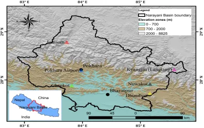
Gandaki, Budhi Gandaki, and Trishuli and it includes Terai, Hill, Mountain and High Himalayas including trans-Himalaya from south to north of the basin. About 40% of the basin is covered by agricultural land [26]. The upper part of this basin covered with snow and ice which is the main source of water. The mean elevation of this basin is 4065 m a.s.l. and ranges from 18 m in the south to higher than 8000 m [28] in the north where the watershed contains the Dhaulagiri (8167 m a.s.l.), Manaslu (>8000 m a.s.l.) and Annapurna (8091 m a.s.l.) peaks, which have very contrasting climates. Langtang, Machhapuchhre, Manaslu, Dhawalagiri and Annapurna mountains in the basin have created the steep variation of climate over the basin.
The average annual precipitation in the Narayani River basin ranges from 152 mm to 5493 mm and 78% of annual precipitation occurs in monsoon (June–September) [27,29]. Lowest precipitation is observed for driest regions including Mustang and Manang located at the leeward-side north of the Annapurna and Lumle receive the highest precipitation [30].
Figure 1.Narayani River basin with the location of the meteorological stations used in this study. The background of the basin shows different elevation zones based on Shuttle Radar Topography Mission Digital Elevation Model.
3. Methods
3.1. Data Availability
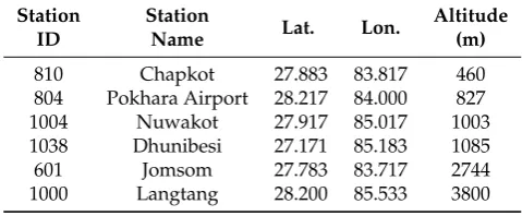
Table 1.Geographic coordinates of the six weather observatories and periods of observations.
Station ID
Station
Name Lat. Lon.
Altitude (m)
810 Chapkot 27.883 83.817 460 804 Pokhara Airport 28.217 84.000 827 1004 Nuwakot 27.917 85.017 1003 1038 Dhunibesi 27.171 85.183 1085 601 Jomsom 27.783 83.717 2744 1000 Langtang 28.200 85.533 3800
Figure 2. Data coverage for the studied stations. Gaps in the lines indicate no available data for the period.
3.2. Basic Statistics
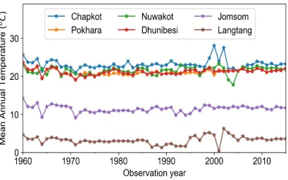
Figure 3.Time series of observed mean annual temperature (◦C) without filling the gap.
Table 2.Distribution of temperature data over six observation station.
Station ID
95th Percentile
99th
Percentile CV Mean Median Skew
Mean after Interpolation
810 28.85 31.68 26.36 23.27 24.77 −0.59 23.20 804 26.38 26.85 21.66 20.96 22.38 −0.46 21.06 1004 26.51 27.88 20.69 21.53 22.86 −0.59 21.45 1038 26.73 27.70 23.71 21.20 22.59 −0.50 21.19 601 18.85 20.77 29.53 11.77 11.68 −0.08 11.44
1000 8.20 9.13 11.29 3.19 3.36 −0.20 3.16
3.3. Quality Control and Data Fill
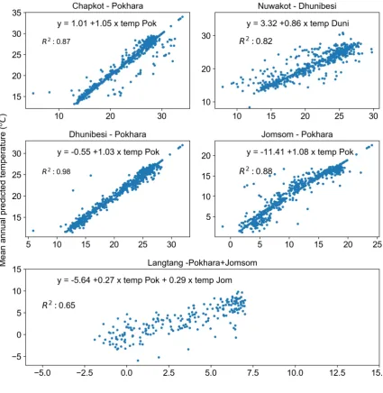
The stepwise option lets us either begin with no variables in the model and proceed forward (adding one variable at a time) or start with all potential variables in the model and proceed backward (removing one variable at a time). At each step, it computes different statistics and selects the best independent variables based on F-test. High R-squared values (>0.80) were observed with less scatter of observed and predicted mean annual temperature around best fit (Figure4) when datasets from Jomsom, Dhunibesi, and Chapkot stations were used as dependent variables and Pokhara as the independent variable. While comparatively smaller value (R2= 0.66) was obtained when data from Langtang station used as dependent variable and data from Pokhara and Jomsom stations as dependent variables. The mean annual temperature after filling the gaps (Figure5) were slightly less than (about 0.10◦C) the mean annual temperature (Table2) before filling the gaps.
Figure 5.Time series plot for annual mean temperature after filling the missing data.
3.4. Trend Break Detection Methods
Empirical mode decomposition (EMD) methods [32,33] which is an adaptive method that is entirely empirical and captures the characteristics, was used for detecting the trend in different periods. Mhamdi et al. [33] have suggested that the EMD can be considered as an attractive and easy method for time series analysis and especially for time series trend extraction and therefore this method was adopted in this study. The key idea of EMD is to locally decompose data into oscillatory components so-called intrinsic mode functions (IMFs). To detect the trend in long-term periods, data from Nuwakot station was used as a representative stations as it has the longest range of dataset as compared to other station datasets.
3.5. Seasonal and Annual trend Analysis
appropriate to identify stations where changes are significant or of large magnitude and to quantify these findings.
3.6. Comparison of Station Data With Freely Available Global Climate Datasets
The gap filled daily mean temperature data from six stations were compared with global climate data sets from freely available sources. For this purpose, WorldClim Version 2.0, CHELSA (Climatologies at high resolution for the earth’s land surface areas) Version 1.2, GLDAS (Global Land Data Assimilation System) Version 2.0 and MODIS (Moderate Resolution Imaging Spectroradiometer) satellite datasets were used.
WorldClim Version 2.0 is a spatially interpolated and gridded climate data for global land areas at a very high spatial resolution (approximately 1 km2) which is based on interpolation methods applied to meteorological station data [40]. The average monthly temperature data for 1970–2000 and ‘Annual Mean Temperature or BIO1 grid from WorldClim Version 2.0 were used in this study. CHELSA Version 1.2 is a high resolution (30 arc sec) climate data set for the earth land surface areas based on a quasi-mechanistical statistical downscaling of the ERA interim global circulation model [41]. The average monthly temperature data for 1979–2013 and ‘Annual Mean Temperature’ grid from CHELSA Version 1.2 were used in this study. GLDAS Version 2.0 uses satellite data products, ground-based observational data products, land surface modeling and data assimilation methods to generate global climate surfaces [42,43]. The parameter ‘near surface air temperature’ in Kelvin from GLDAS Noah Land Surface Model L4 monthly 0.25×0.25 degree Version 2.0 datasets were used in this study.
MOD11A2 Version 6.0 product, one of the several MODIS satellite products, was used in this study. MOD11A2 Version 6.0 provides an average, 8-day, per-pixel land surface temperature (LST) in a 1200×1200 kilometer grid where each pixel value has a spatial resolution of 1 kilometer and the pixel value is a simple average of all the corresponding MOD11A1 LST pixels collected within that 8 day period. LST daytime and LST nighttime were extracted from the MOD11A2 grid for all six stations and separately averaged to obtain monthly average LST daytime and monthly average LST nighttime. Monthly averages of LST daytime and LST nighttime were further averaged to obtain monthly average LST for all months at all six stations. Since a single grid represents the 8-day average, a grid which is averaged using 8 days from two adjacent months was placed in the month with larger number of days used to create the 8-day average grid. Further, when a grid was averaged using equal or 4 days in two adjacent months, the grid was placed in both months to create the monthly average. As data from these sources are freely available in the form of grids, these grids were uploaded as raster data in ArcMap 10.5. The grids and station coordinates were projected into the same geographic projection using the WGS-84 datum and the function ‘Extract Multi Values to Points’ in ArcMap was used to extract the pixel values at station coordinates. Raster Calculator function in ArcMap 10.5 was used to convert digital number values of MOD11A2 grid into degree Celsius and also to convert temperatures in Kelvin in GLDAS 2.0 data set to degree Celsius.
For comparison with WorldClim 2.0 monthly averages and annual mean temperature, station data from 1970 to 2000 were used to generate monthly averages and mean annual air temperature (MAAT hereafter). Similarly, for comparison with CHELSA Version 1.2 monthly averages and annual mean temperature, station data from 1979 to 2013 were used to generate monthly averages and MAAT. For comparison with GLDAS Version 2.0 monthly averages, GLDAS Version 2.0 monthly temperature data set ranging from 2001–2010 and station data from 2001 to 2010 were used to generate monthly averages and MAAT. For comparison of MOD11A2 Version 6.0 product with station data, MOD11A2 Version 6.0 for the year 2015 was compared with station data for the year 2015. Further, GLDAS Version 2.0 monthly temperature data set for the year 2015 was also used for comparison.
4. Results and Discussion
4.1. Trend Break Observation
EMD methods were used for detecting temperature trends in six stations within Narayani River basin. Intrinsic mode functions (IMFs) 1 exhibit high frequency and can represent very short-term fluctuation (Figure6), IMFs 2–3 captures small percentage of variance, IMFs 4–5 capture mid-term effects described by periodic cyclic variation [44]. Finally, IMF 6, the residue component in EMD could represent the major trend [45] of annual average temperature in the long term that may be related with the increase or decrease of observed temperature in Pokhara station. The annual average temperature is in a decreasing trend till 1972 and it breaks there and again the trend is in an increasing order and represents the major trend of temperature (Figure6). It may be related with rapid global warming after the 1970s with industrial evolution and increase of greenhouse gases (GHGs) and radiative forcings [2]. The small difference in a number of year of trend break might be attributed to the influence of local and regional climate.
4.2. Historical Observed Trend
The observed historical mean annual temperature anomaly after filling the gaps for the period of 1960–2015 are shown in Figure5. This dataset represents the basis for calculation of the annual and seasonal trend for each station. Few extreme events of temperature rise and fall are recorded in the data and also shows spatial variability in temperature as stations are located in different physiographic zones. The average annual temperature of the basin is 16.92◦C, however, temperature varies largely with altitude.
Figure 7.Historical mean annual temperature trend in Narayani river basin for six stations. The trend line for the earlier period for each station is denoted by black lines and later period is denoted by blue lines, while the overall trend is denoted by red lines.
Table 3.Mean annual temperature trend (◦C per year) in Narayani River basin at six different stations. ’*’ represents statistically significant at 95% significant level.
SN Station
Name First Half Second Half Entire Period
Date Temp.
Trend Date
Temp.
Trend Date
Temp. trend
1 Chapkot 1960–1972 −0.2207 * 1973–2015 0.0168 1960–2015 0.0009
2 Pokhara
Airport 1960–1970 −0.2110 * 1971–2015 0.0354 * 1960–2015 0.0102 * 3 Nuwakot 1960–1972 −0.2145 1973–2015 0.0280 * 1960–2015 0.0152 * 4 Dhunibesi 1960–1972 −0.2145 * 1973–2015 0.0280 * 1960–2015 0.0080 * 5 Jomsom 1960–1970 −0.0790 1971–2015 0.0294 * 1960–2015 0.0016 6 Langtang 1960–1992 −0.0550 * 1993–2015 0.0410 1960–2015 0.0107
results are also shown by Kattel and Yao [20] and You et al. [4], and it might be possibly due to the small number of stations at different elevation zones. It needs to be verified using several stations in the region.
Results obtained from the Mann-Kendall test for Pokhara and Dhunibesi stations revealed a significant cooling trend during the period ranging from 1960 to 1970–1972, which is similar to previous findings e.g., Liu et al. [23], Shrestha et al. [18] and others. Similarly, a statistically significant cooling trend was also observed at Langtang station for the period from 1960–1992. The mean cooling trend for Pokhara, Chapkot, Dhunibesi, and Langtang station was−0.18◦C per year, however, cooling trend is not very significant for Jomsom and Nuwakot station in the studied period.
4.3. Seasonal Trends
The mean monthly temperature for the study period at each station (Figure8) shows the lowest mean temperature in January, while maximum temperature in all stations was observed during June–August. Minimum mean monthly temperature was found lowest at Langtang station (−0.88◦C) followed by Jomsom station (3.71◦C) in January. Maximum mean monthly temperature was found at Chapkot station (28.31◦C) in August followed by Dhunibesi station (26.20◦C) in June. To get a better overview of the data spread from the mean, monthly average temperature variance (square of the standard deviation) for each station was calculated (Figure9). Higher variance of monthly average temperature was observed in the month of April and December compared to other months. April indicates the transition between winter and summer month. Higher monthly mean variance in April is the indicator for changing the number of days in winter and summer. Hanjra and Qureshi [47], KC and Ghimire [48] also observed more frequent warmer days and less frequent cooler nights throughout Nepal. Annual maximum temperature is in an increasing trend with hot summer days while minimum temperature is in decreasing trend with cool winter days [49] which is reflected by the higher variance in the month of April and December.
Figure 8.Monthly averaged temperature for six station in Narayani basin.
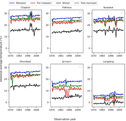
Figure 10.Historical mean seasonal temperature trend in Narayani river basin for six stations.
Table 4.Mean seasonal temperature trend (◦C per year) in Narayani River basin at six different stations from 1970–2015. ’*’ represents statistically significant at 95% significant level.
Station ID
Station
Name Date Monsoon Winter Pre-Monsoon Post-Monsoon
1 Chapkot 1970–2015 0.021 0.019 0.027 0.021 *
2 Pokhara
Airport 1970–2015 0.037 * 0.038 * 0.034 * 0.036 * 3 Nuwakot 1970–2015 0.03 * 0.021 * 0.03 * 0.036 * 4 Dhunibesi 1970–2015 0.038 * 0.024 * 0.037 * 0.039 * 5 Jomsom 1970–2015 0.051 * 0.057 * −0.0080 0.014 6 Langtang 1970–2015 0.042 * 0.038 * 0.015 0.027 *
4.4. Temperature Gradients
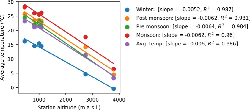
regression between mean temperature and elevation and were found to be−0.0060◦C per m with high value of coefficient of determination (Figure11), which is similar to values reported by Baral et al. [24], Immerzeel et al. [14], Takahashi [50] in the Langtang Valley of the same basin. Steepest temperature gradient (−0.0064◦C per m) was observed during the pre-monsoon season is also consistent with observations from Baral et al. [24], Immerzeel et al. [51] in Langtang Valley, a mountainous part of Narayani basin. Highest (−0.0052◦C per m) and less negative temperature gradient was observed during the winter season, whereas post-monsoon and monsoon season shows the same value of lapse rates (−0.0062◦C per m). However, very high lapse rates of−0.0013◦C per m and−0.0009◦C per m for the monsoon and winter season, respectively were reported by Chand et al. [52] between Langtang station and Lirung debris-covered glacier located at about 4100 m a.s.l. The discrepancies between different seasons are due to differences in relative humidity [51]) and incoming solar radiation [24]. The very less steep gradients of temperature between the debris-covered glacier and low land areas are due to strong influence of surface heating during daytime to near-surface air temperature [52]. It indicates a strong relationship between temperature and elevation and is useful for prediction of temperature for high mountain areas, where there is lack of observation. However, lapse rates may also vary according to land use type [53].
Figure 11. The mean temperature at six stations plotted against elevation for the entire period (1960–2015), winter, post-monsoon, pre-monsoon and monsoon period.
4.5. Comparison of Station Data With Freely Available Global Climate Datasets
Figure 12. Comparison of mean monthly temperature and MAAT from WorldClim 2.0, CHELSA Version 1.2, station data (1970-2000), station data (1979-2013), station data (2001-2010) and GLDAS 2.0 data sets. The numbers 1-12 in X-axis represent months in a year where 1 means January and 12 means December. The alphabet M in X-axis represents MAAT. Values in Y-axis represent temperature in degree Celsius.
Figure 13. Comparison of LST (daytime), LST (nighttime), LST (average), station data (2015) and GLDAS 2.0 data (2015) for all six stations. The numbers 1-12 in X-axis represent months in a year where 1 means January and 12 means December. Values in Y-axis represent temperature in degree Celsius.
Linearly fitted trend lines in scatterplots between mean monthly averages and MAAT values from CHELSA 1.2 and station data (1979–2013) show significant correlation (R2 > 0.94) between the two datasets for all stations (Figure15).
Linearly fitted trend lines in scatterplots between mean monthly averages from GLDAS 2.0 (2001–2010) and station data (2001–2010) show significant correlation (R2 > 0.94) between the two datasets for Jomsom, Dhunibesi and Pokhara while a satisfactory correlation between the two datasets for Nuwakot (R2= 0.78) and Chapkot (R2= 0.73) (Figure16).
Linearly fitted trend lines in scatterplots between mean monthly averages from MOD11A2 LST average of daytime and nighttime values (2015) and station data (2015) show a significant correlation (R2 > 0.94) between the two datasets for Nuwakot, Chapkot and Dhunibesi while a satisfactory
correlation between the two datasets for Jomsom (R2 = 0.89), Pokhara (R2 = 0.79) and Langtang (R2= 0.76) (Figure17).
Overall, the gap-filled data after interpolation is in good agreement with climate datasets from different freely available sources.
Figure 15.Scatterplot between CHELSA 1.2 and station dataset (1979–2013) for all six stations with fitted linear trend lines. Values in X-axis and Y-axis represent temperature in degree Celsius. The equation of linear regression and R-squared values for all six stations are shown in the figure.
Figure 17.Scatterplots between MOD11A2 LST (average) and station dataset (2015) for all six stations with fitted linear trend lines. Values in X-axis and Y-axis represent temperature in degree Celsius. The equation of linear regression and R-squared values for all six stations are shown in the figure.
5. Conclusions
This study contributes to the understanding of annual and seasonal temperature trends for the last fifty years (1960–2015) and several intermediate periods in the Narayani river basin of Nepal. It also demonstrates that the application of simple and multiple linear regression methods with ordinary least squares assumption is efficient to fill gaps in temperature datasets. Gap-filled daily mean temperature dataset is prepared for the duration 1960–2015. Further, this study applied EMD to find out the trend break and Mann-Kendall test to assess the mean temperature trend. An acceptable correlation between the gap-filled data after interpolation with temperature datasets from different freely available sources enhances the reliability upon the gap-filling procedure. Simultaneously, it also suggests that freely available temperature data sources can be equally useful for studies in mountain river basins where station-based data sources are scarce.
Based on analysis of long-term temperature data sets from six different stations located within the Narayani River basin, this study observed the following:
1. The mean annual temperature trend shows a trend break in 1970s for most of the stations. After 1970s, the mean temperature increased at a statistically significant rate in the majority of stations. 2. The rate of increase of mean annual temperature ranges from 0.028◦C to 0.035◦C per year with
mean warming trend of 0.03◦C per year.
3. The highest increase in annual temperature is recorded in monsoon season followed by winter season, post-monsoon season and pre-monsoon season, respectively.
4. The temperature lapse rate with altitude is 0.006◦C per m in the Narayani River basin with the steepest value in pre-monsoon season.
5. The relation between temperature and elevation is significant and very useful for temperature prediction in the higher Himalayan region where observations are scarce.
inclusion of other available observed, reanalysis, and satellite datasets for this basin can be very useful to represent each micro-climatic zone within this basin.
Author Contributions:M.B.C. and B.C.B. designed the analysis. M.B.C. and B.C.B. performed the experiments, and analyzed the data. M.B.C. and B.C.B. wrote the manuscript with input from Prashant Baral and Niraj Shankar Pradhananga.
Acknowledgments:We are thankful to the Department of Hydrology and Meteorology, Government of Nepal (DHM,GoN) for providing a massive data.
Conflicts of Interest:The authors declare that they have no conflict of interest.
References
1. Safari, B. Trend Analysis of the Mean Annual Temperature in Rwanda during the Last Fifty Two Years.JEP
2012,3, 538–551, doi:10.4236/jep.2012.36065.
2. IPCC.Climate Change 2014: Synthesis Report. Contribution of Working Groups I, II and III to the Fifth Assessment Report of the Intergovernmental Panel on Climate Change; Technical Report; IPCC: Geneva, Switzerland, 2014. 3. Hansen, J.; Ruedy, R.; Sato, M.; Lo, K. GLOBAL SURFACE TEMPERATURE CHANGE.Rev. Geophys.2010,
48, doi:10.1029/{2010RG000345}.
4. You, Q.; Kang, S.; Pepin, N.; Flügel, W.A.; Sanchez-Lorenzo, A.; Yan, Y.; Zhang, Y. Climate warming and associated changes in atmospheric circulation in the eastern and central Tibetan Plateau from a homogenized dataset. Glob. Planet. Chang.2010,72, 11–24, doi:10.1016/j.gloplacha.2010.04.003.
5. Yang, K.; Ye, B.; Zhou, D.; Wu, B.; Foken, T.; Qin, J.; Zhou, Z. Response of hydrological cycle to recent climate changes in the Tibetan Plateau. Clim. Chang.2011,109, 517–534, doi:10.1007/s10584-011-0099-4.
6. Hamid, A.; Sharif, M.; Archer, D. Analysis of Temperature Trends in Sutluj River Basin, India. J. Earth Sci. Clim. Chang.2014,5, 222.
7. Bajracharya, S.R.; Maharjan, S.B.; Shrestha, F.; Guo, W.; Liu, S.; Immerzeel, W.; Shrestha, B. The glaciers of the Hindu Kush Himalayas: Current status and observed changes from the 1980s to 2010.Int. J. Water Resour. Dev.2015,31, 161–173, doi:10.1080/07900627.2015.1005731.
8. Bolch, T.; Kulkarni, A.; Kääb, A.; Huggel, C.; Paul, F.; Cogley, J.G.; Frey, H.; Kargel, J.S.; Fujita, K.; Scheel, M.; et al. The state and fate of Himalayan glaciers. Science2012,336, 310–314, doi:10.1126/science.1215828. 9. Lama, L.; Kayastha, R.B.; Maharjan, S.B.; Bajracharya, S.R.; Chand, M.B.; Mool, P.K. Glacier area and volume
changes of Hidden Valley, Mustang, Nepal from ˜1980s to 2010 based on remote sensing. Proc. IAHS2015,
368, 57–62, doi:10.5194/piahs-368-57-2015.
10. Ageta, Y.; Iwata, S.; Yabuki, H.; Naito, N.; Sakai, A.; Narama, C.; Karma. Expansion of glacier lakes in recent decades in the Bhutan Himalayas. InDebris-Covered Glaciers; Nakawo, M., Raymond, C.F., Fountain, A., Eds.; International Association of Hydrological Sciences: London, UK, 2000; Volume IAHS Publication no. 264, pp. 165–175.
11. Khanal, N.R.; Hu, J.M.; Mool, P. Glacial lake outburst flood risk in the poiqu/bhote koshi/sun koshi river basin in the central himalayas. Mt. Res. Dev.2015,35, 351–364, doi:10.1659/{MRD}-{JOURNAL}-D-15-00009. 12. Nie, Y.; Liu, Q.; Liu, S. Glacial lake expansion in the central Himalayas by Landsat images, 1990–2010.
PLoS ONE2013,8, e83973, doi:10.1371/journal.pone.0083973.
13. Gruber, S.; Fleiner, R.; Guegan, E.; Panday, P.; Schmid, M.O.; Stumm, D.; Wester, P.; Zhang, Y.; Zhao, L. Review article: Inferring permafrost and permafrost thaw in the mountains of the Hindu Kush Himalaya region. Cryosphere2017,11, 81–99, doi:10.5194/tc-11-81-2017.
14. Immerzeel, W.W.; van Beek, L.P.H.; Bierkens, M.F.P. Climate change will affect the Asian water towers.
Science2010,328, 1382–1385, doi:10.1126/science.1183188.
15. Yang, X.; Zhang, T.; Qin, D.; Kang, S.; Qin, X. Characteristics and Changes in Air Temperature and Glacier’s Response on the North Slope of Mt. Qomolangma (Mt. Everest).Arct. Antarct. Alp. Res.2011,43, 147–160. 16. Duan, A.; Xiao, Z. Does the climate warming hiatus exist over the Tibetan Plateau?Sci. Rep.2015,5, 13711,
doi:10.1038/srep13711.
18. Shrestha, A.B.; Wake, C.P.; Mayewski, P.A.; Dibb, J.E. Maximum Temperature Trends in the Himalaya and Its Vicinity: An Analysis Based on Temperature Records from Nepal for the Period 1971–94.J. Clim.1999,
12, 2775–2786, doi:10.1175/1520-0442(1999)012<2775:MTTITH>2.0.CO;2.
19. Khatiwada, K.; Panthi, J.; Shrestha, M.; Nepal, S. Hydro-Climatic Variability in the Karnali River Basin of Nepal Himalaya.Climate2016,4, 17, doi:10.3390/cli4020017.
20. Kattel, D.B.; Yao, T. Recent temperature trends at mountain stations on the southern slope of the central Himalayas.J. Earth Syst. Sci.2013,122, 215–227, doi:10.1007/s12040-012-0257-8.
21. Nepal, S. Impacts of climate change on the hydrological regime of the Koshi river basin in the Himalayan region. J. Hydro-Environ. Res.2016,10, 76–89, doi:10.1016/j.jher.2015.12.001.
22. Shrestha, A.B.; Bajracharya, S.R.; Sharma, A.R.; Duo, C.; Kulkarni, A. Observed trends and changes in daily temperature and precipitation extremes over the Koshi river basin 1975-2010. Int. J. Climatol.2017,
37, 1066–1083, doi:10.1002/joc.4761.
23. Liu, Z.; Yang, M.; Wan, G.; Wang, X. The Spatial and Temporal Variation of Temperature in the Qinghai-Xizang (Tibetan) Plateau during 1971–2015. Atmosphere2017,8, 214, doi:10.3390/atmos8110214. 24. Baral, P.; Kayastha, R.B.; Immerzeel, W.W.; Pradhananga, N.S.; Bhattarai, B.C.; Shahi, S.; Galos, S.; Springer,
C.; Joshi, S.P.; Mool, P.K. Preliminary results of mass-balance observations of Yala Glacier and analysis of temperature and precipitation gradients in Langtang Valley, Nepal. Ann. Glaciol. 2014, 55, 9–14, doi:10.3189/2014AoG66A106.
25. Ren, G.Y.; Shrestha, A.B. Climate change in the Hindu Kush Himalaya. Adv. Clim. Chang. Res. 2017,
8, 137–140, doi:10.1016/j.accre.2017.09.001.
26. Dahal, P.; Shrestha, N.S.; Shrestha, M.L.; Krakauer, N.Y.; Panthi, J.; Pradhanang, S.M.; Jha, A.; Lakhankar, T. Drought risk assessment in central Nepal: Temporal and spatial analysis. Nat. Hazards2016,80, 1913–1932, doi:10.1007/s11069-015-2055-5.
27. Panthi, J.; Dahal, P.; Shrestha, M.; Aryal, S.; Krakauer, N.; Pradhanang, S.; Lakhankar, T.; Jha, A.; Sharma, M.; Karki, R. Spatial and Temporal Variability of Rainfall in the Gandaki River Basin of Nepal Himalaya.
Climate2015,3, 210–226, doi:10.3390/cli3010210.
28. Gurung, D.R.; Maharjan, S.B.; Shrestha, A.B.; Shrestha, M.S.; Bajracharya, S.R.; Murthy, M.S.R. Climate and topographic controls on snow cover dynamics in the Hindu Kush Himalaya. Int. J. Climatol. 2017,
37, 3873–3882, doi:10.1002/joc.4961.
29. Bhattarai, B.C.; Regmi, D. Impact of Climate Change on Water Resources in View of Contribution of Runoff Components in Stream Flow: A Case Study from Langtang Basin, Nepal. J. Hydrol. Meteorol.2016,9, 74, doi:10.3126/jhm.v9i1.15583.
30. Karki, R.; Hasson, S.; Schickhoff, U.; Scholten, T.; Böhner, J. Rising Precipitation Extremes across Nepal.
Climate2017,5, 4, doi:10.3390/cli5010004.
31. Leys, C.; Ley, C.; Klein, O.; Bernard, P.; Licata, L. Detecting outliers: Do not use standard deviation around the mean, use absolute deviation around the median. J. Exp. Soc. Psychol. 2013, 49, 764–766, doi:10.1016/j.jesp.2013.03.013.
32. Huang, N.E.; Shen, Z.; Long, S.R.; Wu, M.C.; Shih, H.H.; Zheng, Q.; Yen, N.C.; Tung, C.C.; Liu, H.H. The empirical mode decomposition and the Hilbert spectrum for nonlinear and non-stationary time series analysis. Proc. R. Soc. A Math. Phys. Eng. Sci.1998,454, 903–995, doi:10.1098/rspa.1998.0193.
33. Mhamdi, F.; Poggi, J.M.; Jaïdane, M. Trend extraction for seasonal time series using ensemble empirical mode decomposition. Adv. Adapt. Data Anal.2011,03, 363–383, doi:10.1142/S1793536911000696.
34. Razavi, T.; Switzman, H.; Arain, A.; Coulibaly, P. Regional climate change trends and uncertainty analysis using extreme indices: A case study of Hamilton, Canada. Clim. Risk Manag. 2016,13, 43–63, doi:10.1016/j.crm.2016.06.002.
35. Xu, Z.; Tang, Y.; Connor, T.; Li, D.; Li, Y.; Liu, J. Climate variability and trends at a national scale. Sci. Rep.
2017,7, 3258, doi:10.1038/s41598-017-03297-5.
36. Kendall, M.G.Rank Correlation Methods, 2nd ed; Charles Griffin: London, UK, 1955.
37. Mann, H.B. Nonparametric tests against trend.Econometrica1945,13, 245, doi:10.2307/1907187. 38. Kendall, M.G.Rank Correlation Methods, 4th ed.; Charles Griffin: London, UK, 1975.
39. Hirsch, R.M.; Slack, J.R.; Smith, R.A. Techniques of trend analysis for monthly water quality data.
40. Fick, S.E.; Hijmans, R.J. WorldClim 2: New 1-km spatial resolution climate surfaces for global land areas.
Int. J. Climatol.2017,37, 4302–4315.
41. Karger, D.N.; Conrad, O.; Böhner, J.; Kawohl, T.; Kreft, H.; Soria-Auza, R.W.; Zimmermann, N.E.; Linder, H.P.; Kessler, M. Climatologies at high resolution for the earth’s land surface areas. Sci. Data2017,4, 170122. 42. Rodell, M.; Houser, P.; Jambor, U.; Gottschalck, J.; Mitchell, K.; Meng, C.J.; Arsenault, K.; Cosgrove, B.; Radakovich, J.; Bosilovich, M.; et al. The global land data assimilation system.Bull. Am. Meteorol. Soc.2004,
85, 381–394.
43. Rui, H.; Beaudoing, H. Readme document for global land data assimilation system version 2 (GLDAS-2) products. GES DISC2011, doi:20120010316.
44. Mahmoud, M.O.M.; Mhamdi, F.; Jaidane-Saidane, M. Long term multi-scale analysis of the daily peak load based on the Empirical Mode Decomposition. In Proceedings of the 2009 IEEE Bucharest PowerTech, Bucharest, Romania, 28 June–2 July 2009; pp. 1–6, doi:10.1109/PTC.2009.5281805.
45. Thapa, A.; Kayastha, R.B. Extraction of Periodic Components and Time Adaptive Long-term Trends of Temperature and Precipitation as Climate Variables in Langtang River Basin, Nepal Using Empirical Mode Decomposition. JCC2015,1, 99–107, doi:10.3233/JCC-150008.
46. Salerno, F.; Guyennon, N.; Thakuri, S.; Viviano, G.; Romano, E.; Vuillermoz, E.; Cristofanelli, P.; Stocchi, P.; Agrillo, G.; Ma, Y.; et al. Weak precipitation, warm winters and springs impact glaciers of south slopes of Mt. Everest (central Himalaya) in the last 2 decades (1994–2013). Cryosphere2015,9, 1229–1247, doi:10.5194/tc-9-1229-2015.
47. Hanjra, M.A.; Qureshi, M.E. Global water crisis and future food security in an era of climate change.
Food Policy2010,35, 365–377, doi:10.1016/j.foodpol.2010.05.006.
48. KC, A.; Ghimire, A. High-Altitude Plants in Era of Climate Change: A Case of Nepal Himalayas. InClimate Change Impacts on High-Altitude Ecosystems; Öztürk, M., Hakeem, K.R., Faridah-Hanum, I., Efe, R., Eds.; Springer International Publishing: Cham, Switzerland, 2015; pp. 177–187, doi:10.1007/978-3-319-12859-7_6. 49. K C, A.; Thapa Parajuli, R.B. Climate change and its impact on tourism in the manaslu conservation area,
nepal. Tour. Plan. Dev.2015,12, 225–237, doi:10.1080/21568316.2014.933122.
50. Takahashi, S. Meteorological features in Langtang Valley, Nepal Himalayas, 1985–1986. Bull. Glacier Res.
1987,5, 35–40.
51. Immerzeel, W.W.; Petersen, L.; Ragettli, S.; Pellicciotti, F. The importance of observed gradients of air temperature and precipitation for modeling runoff from a glacierized watershed in the Nepalese Himalayas.
Water Resour. Res.2014,50, 2212–2226, doi:10.1002/{2013WR014506}.
52. Chand, M.B.; Kayastha, R.B.; Parajuli, A.; Mool, P.K. Seasonal variation of ice melting on varying layers of debris of Lirung Glacier, Langtang Valley, Nepal.Proc. IAHS2015,368, 21–26, doi:10.5194/piahs-368-21-2015. 53. Parajuli, A.; Chand, M.B.; Kayastha, R.B.; Shea, J.M.; Mool, P.K. Modified temperature index model for estimating the melt water discharge from debris-covered Lirung Glacier, Nepal. Proc. IAHS2015,
368, 409–414, doi:10.5194/piahs-368-409-2015.
c