Efficient priority rules for dynamic sequencing with sequence-dependent setups Pages 367-384 Download PDF

(1)

International Journal of Industrial Engineering Computations 7 (2016) 367–384

Contents lists available at GrowingScience

International Journal of Industrial Engineering Computations

homepage: www.GrowingScience.com/ijiec

Efficient priority rules for dynamic sequencing with sequence-dependent setups

A. S. Xanthopoulosa*_{, D. E. Koulouriotis}a_{, A. Gasteratos}a_{and S. Ioannidis}b

a_{Department of Production & Management Engineering, Democritus University of Thrace, V. Sofias 12, 67100, Xanthi, Greece} b_{School of Production Engineering & Management, Technical University of Crete, TUC University Campus, 73100, Chania, Greece}

C H R O N I C L E A B S T R A C T

Article history:

Received November 4 2015 Received in Revised Format December 21 2015 Accepted February 10 2016 Available online

February 12 2016

This article addresses the problem of dynamic sequencing on n identical parallel machines with stochastic arrivals, processing times, due dates and sequence-dependent setups. The system operates under a completely reactive scheduling policy and the sequence of jobs is determined with the use of dispatching rules. Seventeen existing dispatching rules are considered including standard and setup-oriented rules. The performance of the system is evaluated by four metrics. An experimental study of the system is conducted where the effect of categorical and continuous system parameters on the objective functions is examined. In light of the results from the simulation experiments, a parameterized priority rule is introduced and tested. The simulation output is analyzed using rigorous statistical methods and the proposed rule is found to produce significantly better results regarding the metrics of mean cycle time and mean tardiness in single machine cases. In respect to three machine cases, the proposed rule matches the performance of the best rule from the set of existing rules which were studied in this research for three metrics.

Keywords: Dynamic sequencing Discrete event simulation Sequence-dependent setups Dispatching rules

1. Introduction

Dynamic scheduling problems with sequence-dependent setups are significantly less well-studied compared with their static counterparts. For example, in a comprehensive survey of scheduling problems with setups by Allahverdi et al. (2008) the case of single-machine with dynamic arrivals is not covered. The review of scheduling problems with sequence-dependent setups by Zhu and Wilhelm (2006) also does not incorporate systems with dynamic arrivals.

(2)

decision-making epoch. A decision-decision-making epoch is a time point where at least one machine is available and there are more than one queueing jobs in the input buffer.

In this environment decisions must be made in real-time, thus the use of dispatching rules for scheduling is a reasonable practice primarily because of its ease of implementation and minimal computational requirements. The performance of a specific dispatching rule varies analogously to the objective function considered and the configuration of the system that it is applied to. Seventeen dispatching rules published in the relevant literature were considered in this study. The set of rules includes standard heuristics such as EDD and SPT, as well as setup-oriented rules (e.g. Vinod & Sridharan, 2008). For the analysis of the system, discrete-event simulation was used. An extended series of simulation experiments was conducted where the effect of categorical and continuous system parameters on four performance metrics was investigated. The insights gained from the analysis of the simulation experiments led to the development of an efficient, parameterized priority rule that was tested extensively. The simulation output was analyzed using rigorous statistical tests and the proposed rule was found to produce excellent results for the metrics of mean WIP, mean cycle time, and mean tardiness.

The structure of the paper is the following. Section 2 contains a brief review of related publications. In Section 3 the dynamic scheduling problem is described. The results from the computer-generated experiments and their analysis are presented in Section 4. The new priority rule is presented and tested in Section 5. The concluding remarks are given in Section 6.

2. Related work

(3)

A. S. Xanthopoulos et al. 3. System description

The description of the dynamic scheduling problem is presented in this section. The system has n identical parallel machines that process m types/groups of jobs (Wang & Liu, 2014) and an input buffer where incoming jobs are stored until they are released for processing. The assumptions made regarding the machines/buffer system are the following: i) there are neither machine failures nor order cancellations, ii) the machines can process only one job at a time, iii) the input buffer has infinite capacity, iv) a job that has completed its processing exits the system immediately, i.e. the machines are never blocked. Table 1 summarizes the nomenclature used in the remainder of the paper.

Table 1 Notation

Notation Description

m number of job types

n number of machines

c job type

 _{mean processing time of jobs}

 mean time between arrivals of jobs

 due date tightness factor



setup factor ofjobs

σj state of machine j (0 and 1 symbolizes idle and working machine, respectively)

l number of queueing jobs

i i-th queueing job in the input buffer

fi number of queueing jobs that belong to the same family with queueing job i

w job type with maximum total processing time in the input buffer

k, j k-th completed job in machine j

) (i

c (c(k, j)) type of i-th queuing (k-th completed on machine j) job

i

a (a_k_,_j) arrival time of i-th queueing (k-th completed on machine j) job

i

p (p_k_,_j) production time of i-th (k-th completed on machine j) queueing job

i

d (dk,j) due date of i-th queueing (k-th completed on machine j) job

j i

s_, (s_k_,_k_₁_,_j) setup time for i-th queueing (k+1- th completed) job on machine j

) (si,j

g penalty for assigning queueing job i to machine j (0 if no setup is required, b otherwise,

where b )

j k

C _, completion time of k-th completed job on machine j



k j k j



j

k d C

E _, max0, _,  _, earliness of k-th completed job on machine j



k j k j



j

k C d

T_, max0, _,  _, tardiness of k-th completed job on machine j

j k j k j

k C d

L_,  _,  _, lateness of k-th completed job on machine j

T time horizon

N total number of completed jobs in T

K set of completed jobs in T

t time

) (t

X WIP at time t, i.e. number of jobs that exist in the system at time t

At time 0, all machines are idle (σj = 0, for all j) and the input buffer is empty (l = 0). Jobs arrive

dynamically to the system at random time intervals with mean



. Processing times of jobs are also stochastic with mean



. The type, processing time, and due date of a job are assumed to become known upon arrival of that job to the system.

The due date of the i-th queueing job satisfies Eq. (1):

i i

i a p

(4)

Sequence-dependent setups (Xanthopoulos et al., 2013) take place when switching from one job type to another in each machine. The length of the setup interval s_k_,_k_₁_,_j for the (k+1)-th completed job in machine j is computed according to Eq. (2):

  

 

 

 

 ₀ _if ₍ _, ₎ ₍ ₁_, ₎

) , 1 ( ) , ( if

, 1 ,

1 ,

j k c j k c

j k c j k c p

s k j

j k k



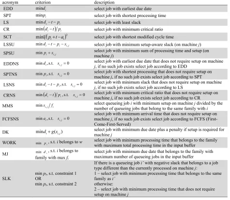
(2)

A job is released for processing whenever a machine is available and the input buffer contains at least one job, i.e. no planned idle time is allowed. Once a machine starts processing a job it cannot be interrupted. At the moment that the currently processed job on machine j is completed the machine’s state shifts from operating to idle. Sequencing is completely reactive, meaning that it is triggered by system-related events. The event that causes a re-sequencing epoch is the transition of a machine’s state from operating to idle provided that the input buffer contains at least two jobs. In a re-sequencing epoch all job priority indices are updated to account for newly arrived jobs. The job priority indices are determined by a dispatching rule that belongs to the set of rules listed in Table 2.

Table 2

Dispatching rules

acronym criterion description

EDD min di select job with earliest due date

SPT min pi select job with shortest processing time

LS minditpi select job with least slack

CR min



dit



pi select job with minimum critical ratio

SCT min1



p_ita_i



2 select job with shortest modified cycle time

LSSU minditpisi,j select job with minimum setup-aware slack (on machine j)

SPSU minpisi,j select job with minimum sum of processing time and setup (on _machine_j₎

EDDNS mind_i,s.t. s_i_,_j0 select job with earliest due date that does not require setup on machine

j, if no such job exists select job according to EDD

SPTNS minpi,s.t. si,j0 select job with shortest processing that does not require setup on _machine_j_{, if no such job exists select job according to SPT}

LSNS mind_itp_i,s.t. s_i_,_j 0 select job with minimum slack that does not require setup on machine

j, if no such job exists select job according to LS

CRNS mindit pi,s.t. si,j 0 select job with minimum critical ratio that does not require setup on _machine_j_{, if no such job exists select job according to CR}

MMS minsi,j fi select queueing job _{number of queueing jobs that belong to the same family with}i with minimum setup on machine j divided by the _i

FCFSNS minai,s.t. si,j0

select job with minimum arrival time that does not require setup on

machine j, if no such job exists select job according to FCFS

(First-Come-First-Served)

DK mind_ig(s_i_,_j) select job with minimum due date plus a penalty if setup is required for

machine j

WORK min pi, s.t. i belongs to w

select job with minimum processing time that belongs to the family with maximum total processing time in the input buffer

MJ min di, s.t. i belongs to

family with max fi

select job with minimum due date that belongs to the family with maximum number of queueing jobs in the input buffer

SLK

min pi, s.t. constraint 1

OR

min pi, s.t. constraint 2

If there is a queueing job i’ with negative slack that belongs to a job

type different than the currently processed on machine j:

1 – select job with minimum processing time that belongs to the same

family as i’

otherwise:

2 – select job with minimum processing time that does not require

setup on machine j

(5)

A. S. Xanthopoulos et al.

 if there is only one queueing job (l = 1) and only one idle machine (with σj = 0), assign the queuing

job to machine j

 if there is only one queueing job and more than one idle machines, assign the queueing job to the machine that does not require setup (if more than one machines do not require setup, ties are broken arbitrarily)

 if there are more than one queueing jobs (l > 1) and only one idle machine (with σj = 0), assign

the job with highest priority according to the dispatching rule in use to machine j

 if there are more than one queueing jobs and more than one idle machines, assign the job with highest priority for idle machine j to machine j. If a queueing job has the highest priority for more than one idle machine, assign it to the machine that does not require setup (if more than one machines do not require setup, ties are broken arbitrarily)

The performance of the system is captured by the following metrics, where  is the cardinality of set operator:

mean WIP:



TX t dt

T 0 ( )

1

(3)

mean cycle time:

 

_j _k Ckj akj

N ( )

1

,

, (4)

mean tardiness:

 

_j _k



C_k _jd_k _j



N max0, , ,

1

(5)

% fraction of tardy jobs:





N T K

k | kj 0

100  ,  (6)

4. Comparison of existing priority rules

The methods described in section 6.1 of Xanthopoulos et al. (2013) were used in order to obtain statistically significant results while controlling the computational cost of the simulation experiments. For each replication of the simulation models, a warm-up period corresponding to 300 completed jobs was used. The parameters of the procedure that controls the length of each independent replication were set to n0 150 and g 0.001, while the parameters of the procedure that controls the number of replications for each simulation model were h0.05 and Kmax 40 (refer to section 6.1 of

Xanthopoulos et al. (2015) for a description of the aforementioned procedures).

We examined 18 simulation cases which are described in Table 3 and Table 4. Cases 1 – 9 pertain to single-machine configurations whereas cases 10–18 concern configurations with three parallel machines.

Table 3

Parameters for simulation cases 1 – 9. The definition of the symbols is given in Table 1

simulation case number

1 2 3 4 5 6 7 8 9

n 1 1 1 1 1 1 1 1 1

m 5 5 5 5 5 5 5 5 5

λ 1.1 1.2 1.3 1.4 1.5 1.4 1.4 1.4 1.4

μ 1.0 1.0 1.0 1.0 1.0 1.0 1.0 1.0 1.0

δ 1.0 1.0 1.0 1.0 1.0 1.0 1.0 1.0 1.0

β 0.1 0.1 0.1 0.1 0.1 0.2 0.3 0.4 0.5

(6)

Table 4

Parameters for simulation cases 10 – 18. The definition of the symbols is given in Table 1

simulation case number

10 11 12 13 14 15 16 17 18

n 3 3 3 3 3 3 3 3 3

m 5 5 5 5 5 5 5 5 5

λ 1.1 1.2 1.3 1.4 1.5 1.4 1.4 1.4 1.4

μ 3.0 3.0 3.0 3.0 3.0 3.0 3.0 3.0 3.0

δ 1.0 1.0 1.0 1.0 1.0 1.0 1.0 1.0 1.0

β 0.1 0.1 0.1 0.1 0.1 0.2 0.3 0.4 0.5

4.1. Comparison of priority rules for varying arrival rates – single machines cases

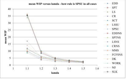
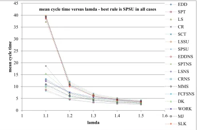
In this section a comparative evaluation of the seventeen priority rules described in Table 2 for single machine cases with varying job arrival rates is conducted. Figs (1-4) show the mean WIP, mean cycle time, mean tardiness and mean percentage of tardy jobs, respectively (y axis) obtained by the 17 priority rules considered in this study versus the mean time between arrivals λ (x axis) for simulation cases 1 - 5. It is observed that the mean WIP, mean cycle time, mean tardiness and mean percentage of tardy jobs decreases monotonically as the mean time between arrivals increases. This is expected since the greater the mean time between arrivals is, the more moderate the workload imposed on the system becomes. In cases where the frequency of arrivals is high, intense queueing effects are monitored and the average time that incoming jobs spend in the system is relatively high.

Fig. 1. Mean WIP for simulation cases 1 - 5

Moreover, exiting jobs are more likely to be tardy than early and so the metrics of mean tardiness and mean percentage of tardy jobs are also at relatively high levels. It is observed that the differences between the various priority rules are more evident in cases where the system is under heavy workload. This is an indication that the performance of the system is mostly affected by the sequencing rule used in cases where it operates close to its maximum attainable throughput rate. The best rule for minimizing mean WIP, mean cycle time and mean tardiness is SPSU for simulation cases 1 - 5.

0 5 10 15 20 25 30 35 40

1 1.1 1.2 1.3 1.4 1.5 1.6

mea

n WI

P

lamda

mean WIP versus lamda - best rule is SPSU in all cases EDD

(7)

Fig. 2. Mean cycle time for simulation cases 1 – 5

Fig. 3. Mean tardiness for simulation cases 1 - 5

The best priority rule for minimizing mean percentage of tardy jobs was found to be SPTNS for cases 2 – 5 and MMS for the first simulation case.

0 5 10 15 20 25 30 35 40 45

1 1.1 1.2 1.3 1.4 1.5 1.6

me

an

cycl

e

ti

me

lamda

mean cycle time versus lamda - best rule is SPSU in all cases EDD_SPT

LS CR SCT LSSU SPSU EDDNS SPTNS LSNS CRNS MMS FCFSNS DK WORK MJ SLK

0 5 10 15 20 25 30 35 40 45

1 1.1 1.2 1.3 1.4 1.5 1.6

mean tardines

s

lamda

mean tardiness versus lamda - best rule is SPSU in all cases

(8)

Fig. 4. Mean percentage of tardy jobs for simulation cases 1 – 5

4.2. Comparison of priority rules for varying levels of setup – single machines cases

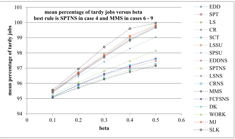
In this section a comparative evaluation of the seventeen priority rules for single machine cases varying levels of the setup factor β is presented. Figs. (5-8) show the performance metrics considered in this study (y axis) obtained by the 17 priority rules versus the setup factor β (x axis) which spans from 0.1 to 0.5 with step size 0.1 (simulation cases 4, 6, 7, 8, 9). It is observed that the due date-oriented priority rules (EDD, LS, LSSU) do not perform satisfactorily in general, whereas the setup-aware rules (EDDNS, SPTNS, LSNS, CRNS, SPSU) excel in respect to their performance for all objective functions. The rules SPT and CR define a somewhat intermediate situation between these two extremes.Increasing the setup magnitude has the effect of slowing down the production process as the averaged total processing time is increased. As a result the mean length of the pending jobs queue, mean cycle time, and mean tardiness is also increased.

Fig. 5. Mean WIP for simulation cases 4, 6, 7, 8, 9

93 94 95 96 97 98 99 100

1 1.1 1.2 1.3 1.4 1.5 1.6

mean per

centa

ge

of tard

y jobs

lamda

mean percentage of tardy jobs versus lamda - best rule is MMS in first case and SPTNS in all other cases

EDD SPT LS CR SCT LSSU SPSU EDDNS SPTNS LSNS CRNS MMS FCFSNS DK WORK MJ SLK

0 50 100 150 200 250

0 0.1 0.2 0.3 0.4 0.5 0.6

mean

WIP

beta

mean WIP versus beta - best rule is SPSU in cases 4, 6 and SPTNS for cases 7, 8, 9 _EDD

(9)

Moreover, priority rules that form batches of jobs that belong to the same class for processing are naturally well-suited for this type of production scenarios as they have the tendency to minimize the frequency of setups.

In respect to the mean WIP and mean cycle time metrics, the SPSU and SPTNS are the best rules for cases 4, 6 and 7 – 9, respectively. Regarding mean tardiness, the best rule is: SPSU for simulation cases 4 and 6, SPTNS for cases 7 and 9, MMS for case 8. Finally, the mean percentage of tardy jobs is minimized by MMS in cases 6 – 9 and by SPTNS in case 4. It is evident that the MMS rule is a good option for due date related performance metrics in situations where the amount of setup is considerable.

Fig. 6. Mean cycle for simulation cases 4, 6, 7, 8, 9

Fig. 7. Mean tardiness for simulation cases 4, 6, 7, 8, 9

This can be attributed to the fact that the MMS rule takes into consideration both the required setup for each queueing job and information on the composition of the set of waiting jobs as a whole.

0 50 100 150 200 250 300

0 0.1 0.2 0.3 0.4 0.5 0.6

me

an

cycl

e

ti

me

beta mean cycle time versus beta

best rule is SPSU in cases 4, 6 and SPTNS for cases 7, 8, 9

EDD SPT LS CR SCT LSSU SPSU EDDNS SPTNS LSNS CRNS MMS FCFSNS DK WORK MJ SLK

0 50 100 150 200 250 300

0 0.1 0.2 0.3 0.4 0.5 0.6

mean tardi

n

ess

beta mean tardiness versus beta - best rule is: SPSU in cases 4, 6 - SPTNS in cases 7, 9 - MMS in case 8

(10)

Fig. 8. Mean percentage of tardy jobs for simulation cases 4, 6, 7, 8, 9

4.3. Comparison of priority rules for varying arrival rates – cases with three parallel machines

In this section the results regarding simulation cases 10 – 14 are presented. It is reiterated that in these cases production systems with three parallel machines are considered and the output of the systems for varying arrival rates is investigated. The performance of the 17 existing priority rules considered in this study are presented in Tables (5–7).

From Tables (5–7) it is observed that the performance of the LSNS rule is matching the performance of the FCFSNS rule. Note that this is because of the due date assignment scheme (Eq. (1)) and not a general property of these two rules.

Simulation cases 10 – 14 are analogous to single machine cases 1 – 5, but they are also differentiated in terms of the magnitude of setup operations. Recall from Eq. (2) that the setup is proportional of the processing time of a job, and that the mean processing time of jobs for cases 10 – 14 is 3.0 compared to the job mean processing time of 1.0 for cases 1 – 5.

Table 5

Results for simulation cases 10 and 11. The minimum values for each performance metric and simulation case are denoted in bold

simulation case 10 simulation case 11

mean WIP mean cycle time

mean tardiness

mean percentage

of tardy jobs mean WIP

mean cycle time

mean tardiness

mean percentage of tardy jobs

EDD 46.73 51.21 48.21 98.91 9.24 11.04 8.04 94.60

SPT 13.23 13.69 10.69 98.87 5.75 6.88 3.87 94.53

LS 47.56 52.17 49.16 98.87 10.74 12.84 9.83 94.63

CR 26.98 29.48 26.48 98.89 7.20 8.61 5.60 94.52

SCT 52.35 57.41 54.40 98.89 12.08 14.44 11.43 94.64

LSSU 56.60 62.19 59.19 99.06 11.53 13.77 10.76 94.88

SPSU 12.02 12.66 9.66 98.64 5.68 6.78 3.77 94.51

EDDNS 13.30 14.54 11.53 96.76 6.65 7.95 4.95 92.91

SPTNS 10.08 11.02 8.01 96.51 5.73 6.86 3.85 92.70

LSNS 14.87 16.26 13.24 96.89 7.41 8.85 5.84 93.19

CRNS 11.01 12.06 9.04 96.66 6.14 7.34 4.33 92.87

MMS 12.13 13.28 10.27 96.44 6.35 7.61 4.60 92.68

FCFSNS 14.87 16.26 13.24 96.89 7.41 8.85 5.84 93.19

DK 16.08 17.58 14.57 97.23 6.76 8.08 5.08 93.17

WORK 15.02 16.07 13.07 98.13 7.97 9.53 6.51 94.06

MJ 50.32 55.17 52.16 98.99 9.59 11.46 8.45 94.58

SLK 57.29 62.66 59.66 99.43 10.58 12.62 9.61 95.49

94 95 96 97 98 99 100 101

0 0.1 0.2 0.3 0.4 0.5 0.6

me

an

perce

ntage of tardy

jobs

beta

mean percentage of tardy jobs versus beta best rule is SPTNS in case 4 and MMS in cases 6 - 9

(11)

As a result the setups in the three machine cases 10 – 14 are lengthier than those of the single machine cases 1 – 5. For that reasons there are some differentiations as to which is the best rule for each performance metric in cases 10 – 14 in comparison to cases 1 – 5. More specifically, the SPTNS rule has the best results in terms of minimizing mean WIP, mean cycle time, and mean tardiness for simulation case 10 where the system operates under heavy workload. For cases 11 – 14 the SPSU rule achieves the best results regarding the aforementioned metrics.

Table 6

Results for simulation cases 12 and 13

mean WIP _{cycle time}mean _tardinessmean mean pct. of _{tardy jobs} mean WIP mean cycle _time _tardinessmean mean pct. of _{tardy jobs}

EDD 5.17 6.70 3.69 90.68 3.83 5.35 2.35 87.28

SPT 4.16 5.39 2.39 90.46 3.42 4.78 1.78 87.21

LS 6.14 7.95 4.94 90.77 4.38 6.11 3.11 87.23

CR 4.76 6.17 3.16 90.82 3.72 5.19 2.18 87.45

SCT 7.01 9.07 6.06 90.78 5.01 6.98 3.97 87.49

LSSU 6.43 8.32 5.31 90.95 4.53 6.34 3.33 87.48

SPSU 4.15 5.39 2.38 90.49 3.38 4.72 1.73 87.01

EDDNS 4.63 6.01 3.01 89.45 3.72 5.19 2.18 86.43

SPTNS 4.28 5.55 2.54 89.31 3.53 4.93 1.93 86.39

LSNS 5.16 6.68 3.67 89.77 3.99 5.58 2.57 86.67

CRNS 4.47 5.80 2.79 89.38 3.64 5.08 2.08 86.47

MMS 4.59 5.95 2.94 89.48 3.66 5.12 2.12 86.28

FCFSNS 5.16 6.68 3.67 89.77 3.99 5.58 2.57 86.67

DK 4.60 5.96 2.95 89.71 3.64 5.09 2.09 86.61

WORK 5.56 7.20 4.19 90.21 4.35 6.06 3.05 86.97

MJ 5.45 7.07 4.05 90.75 4.05 5.65 2.64 87.29

SLK 5.75 7.45 4.44 91.18 4.26 5.93 2.92 87.87

Table 7

Results for simulation case 14. The minimum values for each performance metric and simulation case are denoted in bold

simulation case 14

mean WIP mean cycle time mean tardiness mean pct. of tardy jobs

EDD 3.14 4.71 1.70 84.26

SPT 2.95 4.42 1.42 84.38

LS 3.53 5.29 2.28 84.41

CR 3.13 4.67 1.66 84.52

SCT 3.95 5.90 2.89 84.50

LSSU 3.60 5.40 2.39 84.48

SPSU 2.94 4.41 1.40 84.28

EDDNS 3.11 4.65 1.65 83.80

SPTNS 3.01 4.50 1.50 83.86

LSNS 3.32 4.97 1.97 83.92

CRNS 3.07 4.59 1.59 83.77

MMS 3.09 4.63 1.62 83.77

FCFSNS 3.32 4.97 1.97 83.92

DK 3.08 4.61 1.60 83.83

WORK 3.54 5.30 2.30 84.01

MJ 3.32 4.96 1.95 84.31

SLK 3.40 5.09 2.08 84.64

In respect to the mean percentage of tardy jobs metric, the MMS and the SPTNS are the best rules for cases 10, 11, 13, 14 and 12, respectively. The performance of the CRNS rule matches that of MMS in case 14 as regards to the mean percentage of tardy jobs.

(12)

Table 8

mean WIP _{cycle time}mean _tardinessmean mean pct. of _{tardy jobs} mean WIP mean cycle _time _tardinessmean mean pct. of _{tardy jobs}

EDD 5.19 7.23 4.23 90.48 8.22 11.48 8.46 93.78

SPT 4.14 5.78 2.78 90.26 5.29 7.38 4.37 93.67

LS 6.05 8.43 5.42 90.59 9.36 13.07 10.06 93.71

CR 4.69 6.55 3.54 90.59 6.52 9.11 6.10 93.60

SCT 6.82 9.50 6.50 90.48 10.36 14.46 11.45 93.68

LSSU 6.67 9.30 6.28 91.06 12.49 17.40 14.39 94.88

SPSU 4.04 5.65 2.64 90.02 4.83 6.748 3.74 92.74

EDDNS 4.15 5.80 2.80 88.52 4.64 6.48 3.47 90.43

SPTNS 3.83 5.37 2.36 88.31 4.22 5.90 2.90 90.11

LSNS 4.58 6.39 3.39 88.81 5.25 7.31 4.30 90.87

CRNS 4.03 5.63 2.63 88.52 4.44 6.20 3.20 90.30

MMS 4.02 5.63 2.62 88.37 4.43 6.20 3.19 90.09

FCFSNS 4.58 6.39 3.39 88.81 5.25 7.31 4.30 90.87

DK 4.16 5.80 2.80 88.75 4.80 6.70 3.69 90.79

WORK 5.23 7.29 4.29 89.59 6.48 9.03 6.02 92.05

MJ 5.50 7.67 4.66 90.55 8.65 12.06 9.05 93.76

SLK 6.00 8.38 5.37 91.33 11.95 16.64 13.63 95.63

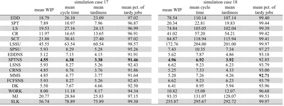
From Table 8 and Table 9 it can be seen that more sophisticated rules such as WORK, MJ, and SLK which utilize information on the entire queueing job set of each job type perform rather poorly. The rationale of the WORK rule is that the frequency of setups is reduced by selecting the job type which will occupy a machine for the longest time. However, this rule tends to prioritize jobs with long processing times and this explains its poor performance. The MJ rule also attempts to reduce the setup frequency by choosing the job type with the largest number of queueing jobs, however as new jobs arrive to the system this practice might actually have a negative effect on the system’s performance. The SLK rule is a truncated version of the SPTNS rule where machines switch between job types based on the slacks of the waiting jobs in the input buffer, nevertheless the experimental results show this intuitive rule to be ineffective in practice.

Simulation cases 15 – 18 are characterized by considerable setup levels, and it can be argued that this is the reason why the SPTNS rule dominates the set of alternative heuristics for the metrics of mean WIP, mean cycle time and mean tardiness. The SPTNS is outperformed only in cases 16 and 18 regarding the mean percentage of tardy jobs by the MMS rule.

Table 9

mean WIP mean

cycle time

mean tardiness

mean pct. of

tardy jobs mean WIP

mean cycle time

mean tardiness

mean pct. of tardy jobs

EDD 18.79 26.10 23.09 97.02 78.54 110.14 107.14 99.40

SPT 7.89 10.97 7.96 96.87 20.34 22.81 19.83 99.44

LS 19.53 27.16 24.15 96.99 74.84 105.05 102.04 99.39

CR 11.97 16.65 13.65 96.91 41.02 57.20 54.21 99.42

SCT 21.88 30.41 27.40 97.02 84.87 118.94 115.94 99.41

LSSU 45.55 63.54 60.54 98.57 172.76 204.00 201.00 99.97

SPSU 5.93 8.29 5.28 95.26 7.43 10.35 7.34 97.27

EDDNS 5.12 7.15 4.15 91.91 5.62 7.87 4.86 93.18

SPTNS 4.55 6.38 3.38 91.46 4.96 6.92 3.92 92.85

LSNS 5.93 8.27 5.26 92.43 6.62 9.23 6.23 93.79

CRNS 4.85 6.76 3.76 91.86 5.25 7.33 4.33 93.00

MMS 4.85 6.77 3.77 91.64 5.20 7.26 4.26 92.71

FCFSNS 5.93 8.27 5.26 92.43 6.62 9.23 6.23 93.79

DK 5.50 7.67 4.66 92.50 6.41 8.95 5.94 93.96

WORK 8.00 11.18 8.17 94.34 10.82 15.08 12.07 96.68

MJ 20.77 28.84 25.83 97.15 93.35 131.07 128.07 99.53

(13)

5. An effective priority rule for dynamic sequencing with sequence-dependent setups

The SPSU rule guarantees that the shortest queueing job is selected for processing at all times. In many cases reported in section 4 and its sub-sections this quality proved to be sufficient for producing the best results. However, the myopic selection of the shortest queueing job is not the best choice in the long run in cases with relatively high setup times, as demonstrated by the results presented in section 4. In many such cases, eliminating setups whenever this is possible and breaking ties based on the minimum processing time in the queue of incoming jobs (SPTNS rule) was found to be the best policy. Furthermore, the SPTNS was found to perform very well in minimizing the mean percentage of tardy jobs. These remarks pave the way for the introduction of a more efficient priority rule which is presented in this

section. The proposed rule PR sequences queueing jobs according to the criterion:

1

min _ si,j _

i b

p (7)

where p_i is the processing time of the i – th queueing job, s_i_,_j is the setup incurred if the i – th is selected for processing on machine j, and b is real positive parameter.

The proposed rule PR is a combination of SPSU and SPTNS. The priority index assigned to a queueing job by SPSU and SPTNS is the sum of its processing time plus a penalty which is a function of the setup needed to process this job. The SPSU uses a linear penalty function and the SPTNS makes use of a step function. The step function eliminates setups provided that its maximum value is sufficiently high. On the other hand, the PR rule utilizes an exponential penalty function. This is demonstrated with an example in Fig. 9.

Fig. 9. Examples of functions for penalizing setups employed by SPSU, SPTNS, and PR

The PR rule resembles the behavior of the SPSU rule for relatively low values of setup and progressively increases the amount of penalty to mimic the behavior of SPTNS for relatively high values of setup time. The growth rate of the penalty function is controlled by adjusting the parameter b.

5.1. Comparison of proposed rule PR to priority rules SPSU, MMS and SPTNS

In this section a comparative evaluation of the PR rule is presented. The methods and parameters to conduct the additional simulation experiments are the same as the ones reported in section 4. The PR rule is compared only to the priority rules which were found to produce the best results (SPSU, SPTNS and MMS) in the simulated cases described in sections 4.1 – 4.4, for brevity. The results for the cases with varying arrival rates and varying setup intensities are presented compactly in Table 10 and Table 11. In order to adjust parameter b of the PR rule the values e (base of the natural logarithm), 3.0, 4.0 and 5.0 were tested and b = 5.0 was ultimately selected. Note that with trivial effort for parameter tuning the PR rule produced very encouraging results. Regarding the mean WIP criterion it is observed that the proposed rule is the best in 9 cases and second to best in 5 cases, out of the 18 simulation cases in total.

setup setup setup

SPSU SPTNS PR

(14)

Table 10

Comparison between SPSU, SPTNS, MMS and PR (continues in Table 11). The minimum values for each performance metric and simulation case are denoted in bold.

single machine cases ( m = 5, μ = 1.0, δ = 1.0 )

3 parallel machine cases ( m = 5, μ = 3.0, δ = 1.0 )

case priority _rule mean WIP mean cycle _time _tardinessmean

mean percentage of tardy jobs mean WIP mean cycle time mean tardiness

λ = 1.1, β

= 0.1

SPTNS 8.76 9.59 8.59 98.61 10.08 11.02 8.01 96.51

SPSU 8.62 8.17 7.18 99.45 12.02 12.66 9.66 98.64

PR(5) 8.56 8.23 7.23 99.43 10.68 11.35 8.36 98.42

MMS 9.99 10.95 9.95 98.60 12.13 13.28 10.27 96.44

λ = 1.2, β

= 0.1

SPTNS 4.71 5.65 4.65 97.28 5.73 6.86 3.85 92.70

SPSU 3.71 4.43 3.43 97.90 5.68 6.78 3.77 94.51

PR(5) 3.63 4.34 3.34 97.87 5.59 6.67 3.66 94.30

MMS 5.06 6.06 5.06 97.30 6.35 7.61 4.60 92.68

λ = 1.3, β

= 0.1

SPTNS 3.11 4.05 3.05 96.14 4.28 5.55 2.54 89.31

SPSU 2.61 3.40 2.39 96.64 4.15 5.39 2.38 90.49

PR(5) 2.60 3.38 2.38 96.63 4.12 5.34 2.34 90.36

MMS 3.37 4.38 3.38 96.17 4.59 5.95 2.94 89.48

λ = 1.4, β

= 0.1

SPTNS 2.38 3.33 2.33 95.06 3.53 4.93 1.93 86.39

SPSU 2.05 2.86 1.86 95.49 3.38 4.72 1.73 87.01

PR(5) 2.05 2.86 1.86 95.42 3.40 4.75 1.74 87.13

MMS 2.50 3.49 2.49 95.08 3.66 5.12 2.12 86.2

λ = 1.5, β

= 0.1

SPTNS 1.92 2.89 1.89 94.11 3.01 4.50 1.50 83.86

SPSU 1.70 2.55 1.55 94.27 2.94 4.41 1.40 84.28

PR(5) 1.70 2.55 1.55 94.24 2.94 4.40 1.39 84.33

MMS 2.04 3.05 2.05 94.20 3.09 4.63 1.62 83.77

In respect to the mean cycle time and the mean tardiness metrics the PR rule ranks first and second in 8 and 6 cases, respectively. The proposed rule performs rather inadequately in terms of the mean percentage of tardy jobs criterion, nevertheless it outperforms the SPSU rule in all simulation cases except two. Table 11

Comparison between SPSU, SPTNS, MMS and PR (continued from Table 10). The minimum values for each performance metric and simulation case are denoted in bold

single machine cases

( m = 5, μ = 1.0, δ = 1.0 )

3 parallel machine cases

( m = 5, μ = 3.0, δ = 1.0 )

case priority _rule mean WIP mean cycle _time _tardinessmean percentage of mean tardy jobs mean WIP mean cycle time mean tardiness

λ = 1.4, β

= 0.2

SPTNS 2.60 3.65 2.65 95.75 3.83 5.37 2.36 88.31

SPSU 2.53 3.55 2.55 96.47 4.04 5.65 2.64 90.02

PR(5) 2.47 3.46 2.46 96.36 3.91 5.46 2.46 89.49

MMS 2.75 3.86 2.86 95.70 4.02 5.63 2.62 88.37

λ = 1.4, β

= 0.3

SPTNS 2.89 4.05 3.05 96.28 4.22 5.90 2.90 90.11

SPSU 3.18 4.45 3.45 97.43 4.83 6.74 3.74 92.74

PR(5) 2.97 4.16 3.15 97.28 4.40 6.15 3.16 91.55

MMS 3.04 4.26 3.26 96.27 4.43 6.20 3.19 90.09

λ = 1.4, β

= 0.4

SPTNS 3.12 4.37 3.37 96.85 4.55 6.38 3.38 91.46

SPSU 3.89 5.45 4.46 98.29 5.93 8.29 5.28 95.26

PR(5) 3.45 4.82 3.82 97.87 4.98 6.96 3.96 93.52

MMS 3.28 4.61 3.60 96.75 4.85 6.77 3.77 91.64

λ = 1.4, β

= 0.5

SPTNS 3.41 4.78 3.78 97.18 4.96 6.92 3.92 92.85

SPSU 5.46 7.50 6.50 99.05 7.43 10.35 7.34 97.27

PR(5) 3.92 5.50 4.50 98.46 5.50 7.68 4.67 94.85

MMS 3.55 4.97 3.97 97.16 5.20 7.26 4.26 92.71

(15)

configuration, a two-way analysis of variance (ANOVA) at the 95% confidence level is carried out to test the effects of the main factors on the response variable. The factors are A) the simulation case (9 levels) and B) the priority rule (4 levels). The ANOVA tests calculate the p-value for the null hypotheses H0A and H0B that observations at all levels of factors A and B are drawn from the same population,

respectively. The results are given in Table 12 and Table 13. Table 12

Two-way ANOVA results for each performance metric (single machine cases).

source SS df F p-value

mean WIP

case 5837.97 8 325.77 0

rule 44.42 3 6.61 0.0002

error 3147.26 1405

mean cycle time

case 4805.3 8 294.66 0

rule 95.38 3 15.6 5.55×10-10

error 2864.11 1405

mean tardiness

case 4807.7 8 298.18 0

rule 95.01 3 15.71 4.69×10-10

error 2831.68 1405

case 2543.41 8 605.75 0

rule 221.1 3 140.42 0

error 737.41 1405

In Table 12 and Table 13, the column labeled ‘source’ describes the source of the variation of the data where ‘case’ is the factor A (the simulation case), ‘rule’ is factor B (the priority rule) and ‘error’ the variability that cannot be attributed to any of the two main factors. The columns labeled ‘SS’, ‘df’, ‘F’ contain the sum of squares, degrees of freedom and F statistic measurements, respectively. Finally, the column labeled ‘p-value’ contains the p-values for the null hypotheses on the main effects. It is observed that the null hypotheses are rejected in all simulation cases (p-values < 0.05).

In order to determine which pairs of means are significantly different, the ANOVA tests are followed-up by multiple comparison procedures (Tukey’s honestly significant difference criterion) for 95% confidence level. The results are illustrated in Figs. (10 – 13).

The plots in Fig.s 10 - 13 depict the population marginal means (Milliken & Johnson, 1992) together with comparison intervals. Marginal means with non-overlapping comparison intervals are significantly different.

Table 13

Two-way ANOVA results for each performance metric (three machine cases)

source SS df F p-value

mean WIP

case 6513.38 8 342.2 0

rule 104.04 3 14.58 2.8×10-9

error 2165.13 910

mean cycle time

case 5574.24 8 301.66 0

rule 149.29 3 21.55 1.73×10-13

error 2101.91 910

mean tardiness

case 5578.74 8 3.09.83 0

rule 149.21 3 22.1 8.1×10-14

error 2048.18 910

case 14152 8 1462.91 0

rule 844.3 3 232.74 0

error 1100.4 910

The results of the follow-up tests for the single machine cases are the following:

(16)

it is inferred that the PR rule outperforms SPSU, SPTNS and MMS in a statistically significant way in respect to the mean cycle time (mean tardiness) metric.

multiple comparison tests – Tukey honestly significant difference criterion – 95% confidence

marginal means with comparison intervals

Fig. 10. Results from multiple comparison follow-up tests for mean WIP and mean cycle time (single

machine cases)

Fig. 11. Results from multiple comparison follow-up tests for mean tardiness and mean percentage of

tardy jobs (single machine cases).

Fig. 12. Results from multiple comparison follow-up tests for mean WIP and mean cycle time (three

machine cases).

Finally, the PR priority rule is significantly better than the SPSU rule and worse than the SPTNS and MMS rules when compared in terms of the mean percentage of tardy jobs as it can be observed in the

3.3 3.5 3.7 3.9 4.1

PR(5) SPSU SPTNS MMS

mean WIP

4.2 4.4 4.6 4.8 5 5.2

mean cycle time

3.2 3.4 3.6 3.8 4 4.2

mean tardiness

96.2 96.4 96.6 96.8 97 97.2 97.4 97.6

4.5 5 5.5 6

mean WIP

6.2 6.7 7.2 7.7

(17)

right-side of Fig. 11. In respect to the results of the follow-up tests for the three machine cases the following observations can be made: Figs. (12-13) indicate that the proposed priority rule achieves significantly better results in comparison to the SPSU and MMS rules for the mean WIP, mean cycle time and mean tardiness metrics. For the aforementioned metrics the performance of PR is statistically equal to that of SPTNS. Similarly to the single machine cases, the PR rule is significantly better than SPSU and worse than SPTNS and MMS in respect to the mean percentage of tardy jobs, for the simulation cases with three machines too.

Fig. 13. Results from multiple comparison follow-up tests for mean tardiness and mean percentage of

tardy jobs (three machine cases). 6. Conclusions

The problem of real-time scheduling on parallel machines with dynamic arrivals, stochastic processing times, due dates and sequence-dependent setups was examined. For the analysis of the system the discrete-event simulation models were used.

A series of simulation experiments involving seventeen dispatching rules was conducted where four performance metrics were considered. The SPSU rule exhibited very good performance in minimizing mean WIP, mean cycle time and mean tardiness in cases with relatively low setup times, whereas in cases with high setup times the SPTNS rule excelled in respect to the aforementioned metrics. The SPTNS and the MMS rules also yielded the best results in minimizing mean percentage of tardy jobs in all cases. Based on the interpretation of the experimental results a parametric priority rule that combines SPSU and SPTNS was introduced and tested in multiple experiments. The simulation output was analyzed using statistical tests and the proposed rule was found to produce significantly better results for the metrics of mean cycle time and mean tardiness in single machine simulation cases. The proposed rule’s output also had statistically insignificant differences regarding the best priority rule in minimizing mean WIP in all cases and mean cycle time and mean tardiness in three machine cases.

The encouraging results of the proposed priority rule were obtained with very little effort regarding its fine-tuning. A plausible direction for future research would be to incorporate a self-adaptive element to the proposed heuristic so as to adjust more effectively to various shop configurations.

References

Adibi, M. A., Zandieh, M., & Amiri, M. (2010). Multi-objective scheduling of dynamic job shop using variable neighborhood search. Expert Systems with Applications, 37(1), 282-287.

Allahverdi, A., Ng, C. T., Cheng, T. C. E., & Kovalyov, M. Y. (2008). A survey of scheduling problems with setup times or costs. European Journal of Operational Research, 187(3), 985-1032.

3 3.5 4 4.5

mean tardiness

90 90.5 91 91.5 92 92.5 93

(18)

Ang, A. T. H., Sivakumar, A. I., & Qi, C. (2009). Criteria selection and analysis for single machine dynamic on-line scheduling with multiple objectives and sequence-dependent setups. Computers & Industrial Engineering, 56(4), 1223-1231.

Arzi, Y., Raviv, D. (1998). Dispatching in a workstation belonging to a re-entrant production line under sequence dependent set-up times. Production Planning & Control, 9(7), 690–699.

Chan, F. T. S., Wong, T. C., & Chan, L. Y. (2006). Flexible job-shop scheduling problem under resource constraints. International Journal of Production Research, 44(11), 2071–89.

Chiang, T.C., Fu, L.C. (2009). Using a family of critical ratio-based approaches to minimize the number of tardy jobs in the job shop with sequence dependent setup times. European Journal of Operational Research, 196 (1), 78–92.

Dominic, P. D. D., Kaliyamoorthy, S.M., & Kumar, S. (2004). Efficient dispatching rules for dynamic job shop scheduling. International Journal of Advanced Manufacturing Technology, 24(1-2), 70-75. Frazier, G.V. (1996). An evaluation of group scheduling heuristics in a flow-line manufacturing cell.

International Journal of Production Research, 34(4), 959–976.

Gavett, J.W. (1965). Three heuristic rules for sequencing jobs to a single production facility. Management Science, 11(8), B166–B176.

Huq, F., Cutright, K., & Bhutta, M. K. S. (2009). The analysis of scheduling rules for non-zero setup costs. International Journal of Technology, Policy and Management, 9(2), 126-147.

Jacobs, F.R., Bragg, D.J. (1988). Repetitive lots: Flow-time reductions through sequencing and dynamic batch sizing. Decision Sciences, 19(2), 281–294.

Kim, S.C., Bobrowski, P.M. (1994). Impact of sequence-dependent setup time on job shop scheduling performance.International Journal of Production Research, 32(7), 1503–1520.

Kim, S.C., Bobrowski, P.M. (1997). Scheduling jobs with uncertain setup times and sequence dependency. Omega, 25(4), 437-44.

Korytkowski, P., Wiśniewski, T., & Rymaszewski, S. (2013). An evolutionary simulation-based optimization approach for dispatching scheduling. Simulation Modeling Practice and Theory, 35, 69-85.

Lee, Y.H., Bhaskaran, K., & Pinedo, M. (1997). A heuristic to minimize the total weighted tardiness with sequence-dependent setups. IIE Transactions, 29(1), 45–52.

Mahmoodi, F., Dooley, K.J. (1991). A comparison of exhaustive and non-exhaustive group scheduling heuristics in a manufacturing cell. International Journal of Production Research, 29(9), 1923–1939. Milliken, G. A., Johnson, D. E. (1992). Analysis of Messy Data, Volume 1: Designed Experiments, Boca

Raton, FL: Chapman & Hall/CRC Press.

Nomden, G., van der Zee, D.J., & Slomp, J. (2008). Family-based dispatching: anticipating future jobs. International Journal of Production Research, 46(1), 73–97.

Pickardt, C. W., Branke, J., (2012). Setup-oriented dispatching rules – a survey, International Journal of Production Research, 50(20), 5823-5842.

Rajendran, C., Holthaus, O., (1999). A comparative study of dispatching rules in dynamic flowshops and jobshops. European Journal of Operational Research, 116(1), 156-170.

Vinod, V., Sridharan, R., (2008). Scheduling a dynamic job shop production system with sequence-dependent setups: An experimental study. Robotics and Computer-Integrated Manufacturing, 24(3), 435-449.

Wemmerlov, U., (1992). Fundamental insights into part family scheduling: the single machine case. Decision Sciences, 23(3), 565–595.

Wilbrecht, J.K., Prescott, W.B., (1969). The influence of setup time on job shop performance. Management Science, 16(4), B274–B280.

Xanthopoulos, A. S., Koulouriotis, D. E., Tourassis, V. D., & Emiris, D. M., (2013) Intelligent controllers for bi-objective dynamic scheduling on asingle machine with sequence-dependent setups. Applied Soft Computing, 13(12), 4704-4717.