A Comparative Evaluation of Snow Depth and Snow Water Equivalent Using Empirical Algorithms and Multivariate regressions

A Comparative Evaluation of Snow Depth and Snow Water

Equivalent Using Empirical Algorithms and Multivariate

regressions

Arash Zaerpour

1

_{, Arash Adib}

1*

_{, Ali Motamedi}

2

1_{Department of Civil Engineering, Engineering Faculty, Shahid Chamran University of Ahvaz, Iran}

2_{Khuzestan Water and Power Authority (KWPA), Ahvaz, Iran}

DOI: https://doi.org/10.30880/ijie.2018.10.01.004

Received 9 October 2017; accepted 1 March 2018, available online 11 March 2018

1. Introduction

Satellite-based remote sensing (RS) techniques can play important role to water resources management, such as investigation on surface water, groundwater, snow and ice, dynamic monitoring of ecology, estimation of water amount necessary for keeping and recovering ecological environment, etc. [1]. A research has incorporated remotely sensed data to forecast streamflow and reservoir storage in the Snake River basin, United States [2]. Also a study integrated RS data using a simple vegetation parameter aggregation method applicable to a distributed rainfall-runoff model [3]. The proposed method provided a reasonably realistic description of area-averaged vegetation nature and characteristics. As well, the root-zone soil moisture (RZSM) was estimated using RS and soil moisture analytical relationship (SMAR) model. Results obtained from remotely sensed data coupled with the SMAR model indicated a good description of RZSM dynamics [4]. Snow as a core component of hydrological cycle is extremely important in runoff generation, soil moisture replenishment, flood risk, etc. Particularly in arid and semi-arid areas, the hydrologic response of the water basins is strongly dependent on the snow conditions. Hence, knowledge of snow conditions can provide crucial information for more sustainable and integrated water resources policies. In this regard, remote sensing technology has been considered as a powerful tool for monitoring snow properties including snow-covered areas (SCA), snow depth (SD), snow water equivalent (SWE), and so on. In the past, snow parameters were monitored using observations made at

scattered points in or around the watersheds. Advances in RS based techniques make it possible to estimate most of snow parameters at both regional and global scales. A research coupled satellite imagery with a distributed snowmelt model for monitoring snow-cover depletion in Quebec, Canada [5]. In this research, a real-time simulation was carried out that resulted in a significant improvement of the timing of flood peak forecast. A research has studied the snow cover variability in a forest ecotone of the United States via moderate resolution imaging spectroradiometer (MODIS) Terra products [6]. Also researchers have utilized RS datasets in order to differentiate among rain, snow, and glacier contributions to river discharge in the western Himalaya [7]. Space borne passive microwave (PM) data are commonly utilized in order to retrieve useful snow parameters [8]. PM radiometer data are promising tools for global monitoring with high temporal repetition rate, because of the potential to observe the earth surface through clouds as well as provide information on the internal properties of the snowpack [9]. Researchers estimated SD from PM data in forest regions of northeast China [10]. In this study, an optimal iteration method was used to retrieve the forest transmissivities at 18 and 36 GHz based on the snow and forest microwave radiative transfer models and the snow properties measured in field experiments.

Brightness temperature (TB) of a snowpack is measured using PM radiometer [11]. A study has improved SD retrieval by integrating microwave TB and visible/infrared reflectance through support vector

machine (SVM) regression [12]. The results

Abstract: Space-borne passive microwave (PM) radiometers have provided an opportunity to estimate Snow water equivalent (SWE) and Snow depth (SD) at both regional and global scales. This study attempts to employ empirical algorithms and multivariate regressions (MRs) using Special Sensor Microwave Imager (SSM/I) brightness temperature (TB) in order to achieve an accurate assessment of SD and SWE which well suited for the interest study area. The SSM/I data consist of Pathfinder Daily EASE-Grid TB supplied by the National Snow and Ice Data Centre (NSIDC). For the present study, satellite-based data were gathered from 1992 through 2015 in two versions (v1: 09 July 1987 to 29 April 2009; v2: 14 December 2006 up to now). The results indicated that a stepwise multivariate nonlinear regression (MNLR) outperformed (r = 0.41, and 0.344 for SD and SWE, respectively) other methods. However, a fairly unsatisfactory correlation between ground-based and satellite derived data has been confirmed due to the sparse ground-based data and not considering other parameters (snow density, moisture, etc.)

A. Zaerpour et al., Int. J. Of Integrated Engineering Vol. 10 No. 1 (2018) p. 23-29

demonstrated that the combination of visible/infrared surface reflectance and microwave TB via SVM regression can provide a more accurate retrieval of SD. There is no single snow algorithm to produce accurate global estimates of SD and SWE [13]. Several Algorithms for SD and SWE estimations, such as [14, 15], they modified method of [13] for forest areas are discussed in the literature. In this regard, empirical formulas are usually easy to use. However, these relationships are closely related to the local conditions of the study area [16]. Statistical methods such as regression analysis, multivariate analysis, and least square approximation models have been deployed in various scientific areas [17]. These methods outperform for extremely small size, and also when a theory indicates a relationship between dependent and independent variables [18]. Scientists compared nonlinear regression (NLR) with a neural network (NN) [19]. Both models provided a comparably good prediction. Further studies have been also conducted by [20, 21] in order to evaluate and predict snow parameters using multivariate regressions, and computational intelligence methods. Their results revealed that NNs outperformed multivariate regression models.

This study aims to compare the empirical formulas for retrieval of SD and SWE proposed by [14, 15], Multivariate linear, and NLR using TB extracted from Multi-frequency Special Sensor Microwave Imager (SSM/I). At last, an appropriate relationship will be developed to monitor the SD and SWE in the study area.

2. Materials and methods

2.1 Brightness Temperature (TB)

Theoretically, TB is an effective temperature of a blackbody radiating the same amount of energy per unit area at the similar wavelengths as the observed body. Empirically, TB is the apparent radiant temperature of a non-blackbody determined by measurement with an optical pyrometer or radiometer. TB at a given

wavelength

 



is the product of the physical

temperature

 

p

T and the emissivity

 

 at a given

wavelength of the surface viewed by the radiometer which can be determined by using equation (1).

 

 

Tp

TB









(1)

Equation (1) is the Rayleigh-Jean approximation of Plank's law for the PM region of the electromagnetic spectrum. It is an approximation and does not take into account the atmosphere effects on the microwave radiation [22].

2.2 SSM/I and Field data

The (SSM/I), flying on board of the Defense Meteorological Satellite Program (DMSP) series satellites is a satellite PM radiometer with the preference over optical and infrared sensors that it can observe large portions of the earth's surface both night and day, through

clouds. The SSM/I system measures TB at seven channels, five frequencies (19, 22, 37, 85, and 91 GHz). All channels operate in both horizontal (H) and vertical (V) polarizations, except for 22GHz fixed at V polarization [16]. In the following text, the channels are abbreviated as 19 H, 19 V, etc.

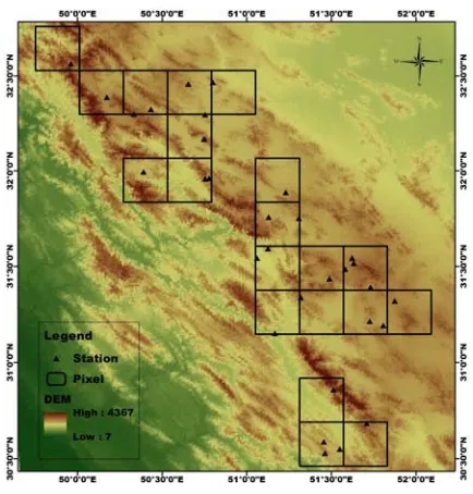
The SSM/I data include Pathfinder Daily EASE-Grid TB supplied by [22]. For the present study, they were gathered from 1992 through 2015 in two versions (v1: 09 July 1987 to 29 April 2009; v2: 14 December 2006 up to now). The temporal resolution is daily and the spatial one is 25km for all channels (19, 22, 37, and 85 GHz), plus 12.5 km for 85 and 91 GHz. The 85 GHz is not available after 29 April of 2009; as well, the 91GHz is only available from the beginning of 2010 [22]. As indicated in Fig. 1, 30 snow stations are located within the study area in which SD and SWE are measured. To increase the reliability of the analysis only pixels with at least one gauge in them were used. In some of the pixels up to three gauges measurements were combined to derive the averaged SD to match EASE-Grid SSM/I spatial resolution. In most basins of Iran, only one or two (even no) snow measurements are recorded at each station during the snowy months in every year. In this study, only 161observation data have been provided for 24 years period (1992-2015).

2.3 Study area

The Upper Karoon River Basin is located in the southwest of Iran extended from 49°-30’ to 52°-15’ longitudes and 30°-23’ to 32°-45’ latitudes with an area

of about 14000 km2 _{(Fig. 1). The elevation ranges from}

2030 m to 4300 m above sea level (asl). Mean annual

temperature and precipitation are 8C and 540 mm. The

majority of the precipitation occurs in winter, mostly from October until May. The main part of this basin is covered with snow for up to five months a year. The highest SD in the study area is 244 cm.

2.4 Empirical algorithms

Researchers proposed an empirical algorithm based on the combination of TB at 18 H and 36 H in order to retrieve the SD and SWE [15]. In this study, the original The Chang et al. (1987) method is applied by replacing 18 H and 36 H with the 19 H and 37 H SSM/I channels, respectively. A revised algorithm was also developed for considering forest cover fraction [13]. As well, a fixed

value of density (0.3 g/cm3_{) was applied to calculate the}

SWE from SD (equation (2)):



H H



C

T

T

R

SWE

SD

,



₁₈



₃₇ (2)

Where, SD and SWE are snow depth (cm) and snow

water equivalent (cm), respectively;

R

_C is a constant

which set to 1.59 cm/K for SD and 4.8 mm/K for SWE

(assuming fixed snow density of 0.3 g/cm3_).

H

T

₁₈ and

H

T

₃₇ are TB (Kelvin) at horizontal polarizations of 18

Fig. 1 Study area with snow stations

The Spectral and Polarization Difference (SPD) algorithm was proposed by Aschbacher (1989) for the retrieval of SD and SWE when no information on the land cover is available. The algorithm is based on a combination of SSM/I channels (equations (3) to (5)):



Tb

V

Tb

V

 

Tb

V

Tb

H



SPD



₁₉



₃₇



₁₉



₁₉        (3)      

Where:

Tb

_XX(H/V) is TB (Kelvin) at

horizontal/vertical polarization for corresponding

frequency.

Equation (3) is used to estimate SD and SWE:

1

0

SPD

A

A

SD







      (4)              



0 1



1

.

0

B

SPD

B

SWE







       (5)       

Where:

A

₀ = 0.68,

A

₁= - 0.67 and

B

₀ = 2.20,

B

₁

= - 7.11 for all data and

A

₀= 0.72,

A

₁ = - 1.24 and

B

₀

= 2.02,

B

₁ = - 7.42 if

T

_max is lower than

0

o

C

.

2.5 Multivariate Regression model

Multivariate linear regression (MLR) is the most common analysis form to explain the relationship between one dependent variable and independent

variables/predictors,

X

_i

(

i



1

,

...,

n

)

. More specifically,

the MLR fits a line through a multi-dimensional cloud of data points. In fact, MLR estimates the coefficients of a linear equation (equation (6)).

n n

X

a

X

a

X

a

a

Y



0



1 1



2 2



...



       (6)

      

Where:

Y

is an estimated value and

a

_i are the

regression coefficients.

Multivariate Nonlinear regression (MNLR) is a method of finding a nonlinear relationship between the

dependent variable and a set of independent variables/predictors. Unlike traditional linear regression restricted to estimating linear models, nonlinear regression is able to evaluate models with arbitrary relationships between independent and dependent variables.

2.6 Methodology

In the study area, ground-based data for SD and SWE should be provided based on measurements conducted in snow stations. As mentioned before, 161 independent measured data are available during 1992-2015. Afterward, the corresponding DMSP SSM/I Pathfinder Daily EASE-Grid TB should be provided for the interest pixels of the study area. Daily TB data in seven channels (19 H, 19V, etc.) have been driven in a flat binary format with 0.1 K precision. TB data values are scaled by 10 which should be divided by 10 to get real Kelvins. The values range from 550 (representing 55.0 K) to 3200 (representing 320.0 K) [22]. For analytic purposes of the present study, the SSM/I seven channels are going to be considered as independent variables. However, the literature has demonstrated that SSM/I high- frequency channels such as 85 and 91GHz do not affect the SD and SWE estimations [13 to 15]. As well, there is a gap in SSM/I data monitoring for 85 and 91 GHz during the study period. Therefore, five channels including (19 H, 19 V, 22 V, 37 H, and 37 V) have been considered as independent/ predictor variables (Table 1).

The pair wise comparisons have been conducted using the Chang et al. (1987) and SPD algorithms. Meanwhile, multivariate analysis of data is performed via the Statistical Package for the Social Science (SPSS) Software for Windows. NR models can be found in [23, 24]. in this regard, we have prepared the following MNLR model (equation (7)):

 



   



 5

1 5

1 5

1

0 j j ij k l kl ik il

i a a X b X X

Y (7)      

Where:

Y

_i is an estimated value of the

i

th observed

data;

a

_j and

b

_kl are the regression coefficients.

Table 1 Selection of the independent variables

Variable Description

X1 Tb19 H

X2 Tb19 V

X3 Tb22 V

X4 Tb37 H

X5 Tb37 V

A. Zaerpour et al., Int. J. Of Integrated Engineering Vol. 10 No. 1 (2018) p. 23-29





 

 

  

n

i i i

n

i i i

Y Y X X

Y Y X X r

1

2 2 1

) ( ) (

) ( )

(       (8)       

n Y X RMSE

n i i i



 

 1

2

)

(       ₍₉₎      

Y X

R       (10)       

Where:

X

_i and

Y

_i are the observed and estimated

values, respectively;

X

and

Y

are the averages of

X

_i

and

Y

_i; n is the whole number of data. (r and R must

close to one and RMSE must close to zero).

3. Results and Discussion

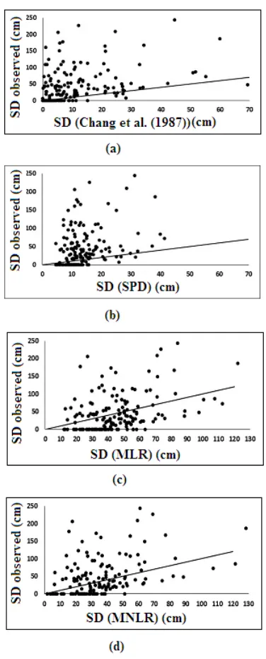
SD and SWE have been estimated using the proposed methods. Fig. 2 shows the estimated versus observed values of SD for four different methods (the Chang et al. (1987), SPD, MLR and MNLR methods).

The correlation coefficient, RMSE, and R are also indicated for each method in Table 2.

Table 2 Correlation coefficient, RMSE, and R for different methods in estimating of SD

SD The Chang et al.

(1987) SPD MLR MNLR

r 0.34 0.3 0.382 0.41

RMSE (cm)

59.63 59.14 48.07 48.83

R 3.98 3.2 1.00 1.31

As indicated in Fig.2, there is not a satisfactory correlation between satellite-derived and ground-based data through different methods, especially for deeper snow depth. This is because that SD exceeds a saturation value that makes the signal emitted from the underlying soil masked. So, deeper SD than saturation depth will not able to be evaluated from PM radiometry leading to underestimation of SD assessments. Moreover, high data shortage for a relatively long period of time (1992-2015) may be another reason for the weak accuracy of results. However, as indicated in Table 2, the highest correlation coefficient belongs to the MNLR method with r = 0.41 (p-value < 0.05) and SPD method has the least value of r (r = 0.3). But, In the case of R, MLR method has the best performance (R= 1.00) while the Chang et al. (1987) method shows the worst value of R (R= 3.98). By observation of RMSE, MLR method has the best performance (RMSE= 48.07 cm) while the Chang et al. (1987) method shows the worst value of RMSE (RMSE= 59.63 cm). By evaluation of three performance criteria, it can conclude that MLR method is the best method in estimating of SD and the Chang et al. (1987) method is the weakest method.

Fig. 2 Observed vs. estimated SD for different methods a) the Chang et al. (1987) b) SPD c) MLR d) MNLR

methods

The relatively better correlation coefficient (0.41) for MNLR may be due to the nonlinear nature of the relationship between SSM/I TB and SD that linear methods cannot represent that. The final MNLR model for SD is obtained using a stepwise regression procedure through SPSS. In this process, some variables were thrown due to the lack of significant contributions to SD (equation (11)):

SD=563.726+4.032X1-0.035 X3+41.017 X4-49.789 X5

describes the correlation between multi-channel frequencies and ground-based SD. Additionally, the choice of suitable starting values is very important. Even if the correct functional form of the model has been specified, poor starting values may fail to converge or get a locally optimal solution rather than one that is globally optimal. Final MLR function is also obtained as follows (equation (12)):

SD=-296.815-0.302X1+4.77 X2-0.386 X3+2.098 X4-4.905

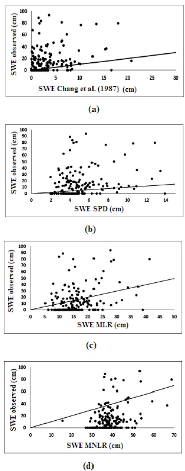
X5 (12) Fig. 3 shows the estimated versus observed values of SWE for different methods. Similar to the SD, there is not a good agreement between observed versus measured SWE values. The low performance of the models in accurate evaluating of SWE may be due to the sensitivity decreasing of the radiometer measurements under deep snow conditions. Moreover, a constant snow density (0.3

g/cm3_{) affects the SWE estimates for different real snow}

conditions.

The correlation coefficient, RMSE, and R are also indicated for each method in Table 3

Table 3 Correlation coefficient, RMSE, and R for different methods in estimating of SWE

SWE The Chang et al.

(1987) SPD MLR MNLR

r 0.28 0.24 0.31 0.344

RMSE

(cm) 23.93 23.37 20.04 30.36

R 4.7 3.16 0.99 0.41

As indicated in Table 3, the highest correlation

coefficient belongs to the MNLR with

r = 0.344 (p-value < 0.05) and SPD has the least value of r (r =0.24). However, In the case of R, MLR has the best performance (R= 0.99) while The Chang et al. (1987) method has the worst value of R (R = 4.7). By observation of RMSE, MLR method has the best performance (RMSE= 20.04 cm) while the MNLR method shows the worst value of RMSE (RMSE= 30.36 cm). By evaluation of three performance criteria, it can conclude that MLR method is the best method in estimating of SWE.

Meanwhile, based on a stepwise MNLR, we have:

SWE=-1421.131+16.033X1+0.377 X3+13.557 X4-18.436

X5-0.034 X12+0.004 X22-0.026 X42+0.033 X52 (13)

And, the LRM is obtained as follows:

SWE=-65.266-0.241X1+1.299 X2+0.156 X3+0.947 X4

-1.858 X5 (14) The relatively low performance of the equations for

both SD and SWE may be due to several reasons. Grain size variation is a significant source of uncertainty [25].

After snow deposits, the constituent crystals

metamorphose in exposing to the vapor gradients within the snowpack or freeze/thaw cycles which is not considered in the present study.

Fig. 3 Observed vs. estimated SWE for different methods a) the Chang et al. (1987) b) SPD c) MLR d) MNLR

methods

A. Zaerpour et al., Int. J. Of Integrated Engineering Vol. 10 No. 1 (2018) p. 23-29

within the sensor footprint because of the complex topography.

4. Conclusion

Several algorithms have been compared to find an appropriate relationship between TB derived from SSM/I and ground-based SD/SWE within the interest study area. Empirical approaches have the advantage of being computationally inexpensive and well suited for large-scale applications. On the other hand, they suffer from the local nature of the coefficients relating SD and SWE to the measured TB. It has been confirmed that TB is not sufficient to accurately evaluate SD and SWE. Other parameters such as snow characteristics (grain size, density, moisture, snow temperature), forest coverage, Topology, etc. should be taken into account to achieve a more realistic estimation of SD/SWE. The results obtained were not fairly satisfactory due to the sparse snow measurements in the study area. Meanwhile, MLR and MNLR models have been developed for the study area which outperforms empirical algorithms. Using of artificial neural network (ANN) and optimization methods as genetic algorithm (GA) can be recognized for overcoming on the problems of inherent nonlinearity relationship between SSM/I data and SD/SWE values.

Acknowledgement

We have especially thanks to Khuzestan Water & Power Authority, Iran, for providing ground- based snow data and NSIDC for making SSM/I data freely available to this research.

References

[1] Li, J. Application of remote sensing to water resources management in arid regions of China. World Water and Environmental resources Congress, (2004), pp. 1-10.

[2] McGuire, M., Wood, A.W., Hamlet, A.F., and Lettenmaier, D.P. Use of satellite data for streamflow and reservoir storage forecasts in the Snake River

basin. Journal of Water Resources Planning and

Management, ASCE, Volume 132(2), (2006), pp. 97-110.

[3] Lee, K.H. Integrating remotely sensed data using a simple vegetation parameter aggregation method applicable to a distributed rainfall-runoff model. Journal of Hydrologic Engineering, ASCE, Volume 13(4), (2008), pp. 236-241.

[4] Faridani, F., Farid, A., Ansari, H., and Manfreda, S. Estimation of the root-zone soil moisture using passive microwave remote sensing and SMAR

model. Journal of Irrigation and Drainage

Engineering,ASCE, Volume 143(1), (2017), pp. 1-9. [5] Lavallée, S., Brissette, F.P., Leconte, R., and

Larouche, B. Monitoring snow-cover depletion by coupling satellite imagery with a distributed

snowmelt model. Journal of Water Resources

Planning and Management, ASCE, Volume 132(2), (2006), pp. 71-78.

[6] Kostadinov, T.S., and Lookingbill, T.R. Snow cover variability in a forest ecotone of the Oregon Cascades

via MODIS Terra products. Remote Sensing of

Environment, Volume 164, (2015), pp. 155-169. [7] Wulf, H., Bookhagen, B., and Scherler, D.

Differentiating between rain, snow, and glacier contributions to river discharge in the western Himalaya using remote-sensing data and distributed

hydrological modeling, Advances in Water

Resources, Volume 88, (2016), pp. 152-169. [8] Singh, D.K., Singh, K.K., Mishra, V.D., and Sharma,

J.K. Formulation of snow depth algorithms for different regions of NW-Himalaya using passive

microwave satellite data. International Journal of

Engineering Research and Technology, Volume 1(5), (2012), pp. 1-9.

[9] Singh, K.K., Mishra, V.D., and Negi, H.S. Evaluation of snow parameters using passive microwave remote

sensing. Defence Science Journal, Volume 57(2),

(2007), pp. 271 - 278.

[10] Che, T., Dai, L., Zheng, X., Li, X., and Zhao, K. Estimation of snow depth from passive microwave brightness temperature data in forest regions of

northeast China. Remote Sensing of Environment,

Volume 183, (2016), pp. 334-349.

[11] Singh, K.K., Kumar, A., Kulkarni, A.V., Datt, P., Dewali, S.K., Kumar, V., and Chauhan, R. Snow depth estimation in the Indian Himalaya using

multi-channel passive microwave radiometer. Current

Science, Volume 108(5), (2015), pp. 942-953. [12] Liang, J., Liu, X., Huang, K., Li, X., Shi, X., Chen,

Y., and Li, J. Improved snow depth retrieval by integrating microwave brightness temperature and

visible/infrared reflectance. Remote Sensing of

Environment, Volume 156, (2015), pp. 500-509. [13] Foster, J.L., Chang, A.T.C., and Hall, D.K.

Comparison of snow mass estimates from a prototype passive microwave snow algorithm, a revised algorithm and a snow depth climatology. Remote Sensing of Environment, Volume 62(2), (1997), pp. 132 - 142.

[14] Aschbacher, J. Land surface studies and atmospheric effects by satellite microwave

radiometry. Ph.D thesis dissertation, University of

Innsbruck, Austria, (1989), 202 p.

[15] Chang, A.T.C., Foster, J.L., and Hall, D.K. Nimbus-7 SMMR derived global snow cover parameters. Annals of Glaciology, Volume 9, (1987), pp. 39 - 44. [16] Tedesco, M., Pulliainen, J., Takala, M., Hallikainen,

M., and Pampaloni, P. (2004). Artificial neural network-based techniques for the retrieval of SWE

and snow depth from SSM/I data. Remote Sensing of

Environment, Volume 90(1), (2004), pp. 76 - 85. [17] Buntine, W.L., and Weigend, A.S. Bayesian

Back-propagation. Complex Systems, Volume 5(6), (1991),

[18] Warner, B., and Misra, M. Understanding neural

networks as statistical tools. The American

Statistician, Volume 50(4), (1996), pp. 284 - 293. [19] Feng, C.X., and Wang, X. Digitizing uncertainty

modeling for reverse engineering applications:

regression versus neural networks. Journal of

Intelligent Manufacturing, Volume 13(3), (2002), pp. 189 - 199.

[20] Tabari, H., Marofi, S., and Abyaneh, H.Z. Comparison of artificial neural network and

combined models in estimating spatial distribution of snow depth and snow water equivalent in Samsami

basin of Iran. Neural Computing and Applications,

Volume 19(4), (2010), pp. 625 - 635.

[21] Marofi, S., Tabari, H., and Abyaneh, H.Z. Predicting spatial distribution of snow water equivalent using multivariate non-linear regression and computational

intelligence methods. Water Resources Management,

Volume 25(5), (2011), pp. 1417-1435.

[22] National Snow & Ice Data Center. (2017). Available at https://nsidc.org/.

[23] Feng, C.X., and Pandey, V. Experimental study of the effect of digitizing parameters on digitizing

uncertainty with a CMM. International Journal of

Production Research, Volume 40(3), (2002), pp. 683 - 697.

[24] Setyawati, B.R., Sahirman, S., and Creese, R.C.

Neural networks for cost estimation. AACE

International Transactions EST13, (2002), pp. 13.1 - 13.8.

[25] Tedesco, M. and Narvekar, P.S. Assessment of the

NASA AMSR-E SWE Product. IEEE Journal of