ISSN: 2393-8366
571
An Energy Efficient Technique For Object
Tracking In Wireless Sensor Networks
R.Radhika1, S.Gowri2, S.Brindha3 1
Research Scholar, St.Peter’s University, Chennai. [email protected]
2
Asst.Prof., Dept. of Computer Science & Applications, St.Peter’s University, Chennai 3
Asst.Prof., Dept. of Computer Science & Applications, St.Peter’s University, Chennai
Abstract: Wireless sensor network (WSN) is distributed over an area and sensors are devoted to task for controlling and monitoring the physical condition of the environment. Interesting application in wireless sensor network isObject Tracking Sensor Network(OTSN)which is used to track the objects in an environment and update its current location to the base station. OTSN accurately detects the location of objects and collecting all the data which is processed and aggregated, sent its current movements to the base station. OTSN is used in several real-life applications like wild-life monitoring, security applications for buildings and international borders monitoring for illegal crossings. There are two major issues in WSN, high energy consumption and low packet delivery rate. Previous object tracking techniques like scheduled monitoring and continues monitoring provides less energy consumption. To improve it, in this proposed system PTSP is used. PTSP has two stages, they are sequential pattern generation and object tracking and monitoring. Effective sleep-awake mechanism is used to conserve energy in proposed system. Markov decision process or learning technique is used to predict the future location of moving objects by mathematical calculations and also reduces object missing rate. Energy calculation and route finding is used to increase the network lifetime. Communication between the sensor node in the network and base station will be based on single-hop communications. The sensor node are static and that the network topology, including the positions of each sensor node in the network, is well known to the base station.
Keywords:OSTN, PTSP, markov decision process
I. INTRODUCTION
Wireless networking which is comprised on number of numerous sensors and they are interlinked or connected with each other for performing the same function collectively or cooperatively for the sake of checking and balancing the environmental factors. This type of networking is called as Wireless sensor networking. A wireless sensor network consists of sensor nodes deployed over a geographical area for monitoring physical phenomena like temperature, humidity, vibrations, and seismic events. Typically, a sensor node is a tiny device that includes three basic components: a sensing subsystem for data acquisition from the physical surrounding environment, a processing subsystem for local data processing and storage, and a wireless communication subsystem for data transmission. In addition, a power source supplies the energy needed by the device to perform the programmed task.
572 II. ISSUES IN SENSOR NETWORK
The issues in wireless sensor network have to be resolved are high energy consumption and low packet delivery rate. Energy conservation is a key issue in the design of systems based on wireless sensor networks. It overcomes the problem in high energy consumption by introducing effective sleep awake mechanism to conserve energy. Energy efficiency is a critical feature of wireless sensor networks (WSNs), because sensor nodes run on batteries that are generally difficult to recharge once deployed. For target tracking one of the most important WSN application type’s energy efficiency needs to be considered in various forms and shapes, such as idle listening, trajectory estimation, and data propagation. A power source supplies the energy needed by the device to perform the programmed task. This power source often consists of a battery with a limited energy budget. In addition, it could be impossible or inconvenient to recharge the battery, because nodes may be deployed in a hostile or unpractical environment. On the other hand, the sensor network should have a lifetime long enough to fulfill the application requirements. In many cases a lifetime in the order of several months, or even years, may be required. External power supply sources often exhibit a non-continuous behavior so that an energy buffer (a battery) is needed as well. In any case, energy is a very critical resource and must be used very sparingly. Therefore, energy conservation is a key issue in the design of systems based on wireless sensor networks.
Object Tracking in Wireless sensor Network (OTSN)
Object tracking is an important application of wireless sensor networks (e.g., military intrusion Detection and habitat monitoring). Existing research efforts on object tracking can be categorized in two ways. In the first category, the problem of accurately estimating the location of an object. In the second category, in-network data processing and data aggregation for object tracking. Object tracking typically involves two basic operations: update and query. In general, updates of an object’s location are initiated when the object moves from one sensor to another. In an OTSN, a number of sensor nodes are deployed over a monitored region with predefined geographical boundaries. The base station acts as the interface between the OTSN and applications by issuing commands and collecting the data of interests. A sensor node has the responsibility for tracking the object intruding its detection area, and reporting the states of the mobile objects with certain reporting frequency, which is adjustable to the network and application requirements. Object tracking sensor networks have two critical operations:
Monitoring:
Sensor nodes are required to detect and track the movement states of Mobile objects.
Reporting
The nodes that sense the objects need to report their discoveries to the applications.
573
Fig. 1.1 Example of OTSN in Wildlife Monitoring
A. Prediction-Based Tracking Technique Using Sequential Pattern Framework
B. In the sequential pattern generation stage, the prediction model is built based on a huge log of data collected from the sensor network and aggregated at the sink in a database, producing the inherited behavioral patterns of object movement in the monitored area. Based on these data, the sink will be able to generate the sequential patterns that will be deployed by the sink to the sensor nodes in the network. This will allow the sensor nodes to predict the future movements of a moving object in their detection area.
C. In the second stage, the actual tracking of moving objects starts. This stage has two parts:
D. Activation Mechanism, which entail the use of the sequential patterns to predict which node(s) should be activated to continually keep tracking of the moving object, and
E. Missing Object Recovery Mechanism, which will be used to find missing objects in case the activated node is not able to locate an object in its detection area.
F. A. Sequential Pattern Generation
G. Sequential Patterns Generation: Definition: The definition of the sequential patterns used in our prediction model following is inspired by the definition of sequential patterns
H. Definition 1: Let S represent the set of sensors in a certain WSN. The list L = [(s1, t1), (s2, t2),
(s3, t3), . . . , (sm, tm)] denotes a list that contains the pairing of each sensor detection
(represented by the sensor ID)and its equivalent time of detection, where si ∈ S and ti <= ti+1 for all 1 <= i < m. The pair (si, ti) represents the detection of a certain event by the sensor si, which took place at time ti. O(L) = [s1, s2, s3, . . . , sm] represents the list of sensors shown in L, except that it was chronologically ordered based on the time of detection recorded by each sensor. O called the list’s sequential pattern.
I. Definition 2: Let DS be a database of sensor lists. The support of the pattern O in DS is defined by the number of lists in DS, where the sequential pattern O represents a subpattern of the lists’ sequential patterns. Thus, Support(O) = |{L ∈ DS|O _ O(L)}|.Therefore, the main goal in mining the sensors’ sequential patterns with a database of lists (DS) and a minimum support (min_sup) is to identify all the sensor sequential patterns that satisfy the user-defined minimum support; these patterns are called frequent sensor sequential patterns.
J. Sequential Patterns and Trisensor Patterns: In our proposed prediction model, to use a special form of sequential patterns, i.e., trisensor patterns. Trisensor patterns can be represented as follows:
574
L. This represents the chronological ordering of the sensors detection of a certain moving object in the network. Therefore, the source sensor represents the sensor ID of the sensor, which detected a particular moving object o before it moved to the next sensor designated as the current sensor; later on, the object o moves to the next sensor denoted by destination sensor. Furthermore, to evaluate the statistical significance of a certain trisensor pattern, we have to calculate the
confidence, in addition to its support, of each particular trisensor pattern. This can be viewed as
the estimate of the probability P(Y |X), which is the probability of finding the right-hand side of the pattern in sequences while these sequences also contain the
M. left-hand side of the pattern. Therefore, the confidence of trisensor pattern. N. [sourcesensor, currentsensor] ⇒ [destinationsensor] is calculated as follows:
Supp([source sensor, current sensor,destination sensor]) Supp([sourse sensor,current sensor])
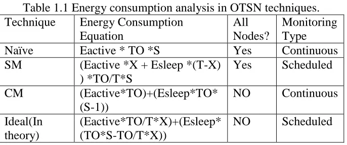
Eactive : The energy consumed by a sensor node per second while its MCU and sensing components are kept in active mode.
Table 1.1 Energy consumption analysis in OTSN techniques. Technique Energy Consumption
Equation
All Nodes?
Monitoring Type Naïve Eactive * TO *S Yes Continuous SM (Eactive *X + Esleep *(T-X)
) *TO/T*S
Yes Scheduled
CM (Eactive*TO)+(Esleep*TO* (S-1))
NO Continuous
Ideal(In theory)
(Eactive*TO/T*X)+(Esleep* (TO*S-TO/T*X))
NO Scheduled
Esieep: The energy consumed by a sensor node per second while its MCU and sensing components are kept in sleep mode.
TO: The total time in seconds in which the OTSN has operated in a continuous manner.
S: Represents all sensor nodes in the network.
X: Represents the sampling duration in milliseconds. During X the sensor is kept in active mode.
T: Represents the period of time in milliseconds which takes place between each report and another sent by a sensor node to the base station.
(T-X): It's the time in milliseconds which begins once a report to the base station was made by the sensor node and lasts until (X) the sampling duration starts. During (T-X) the sensor node is kept in sleep mode.
To/T: This is the total number of reports during the entire network's operational period.
III RESULTS
Missing Object Recovery Mechanism
575
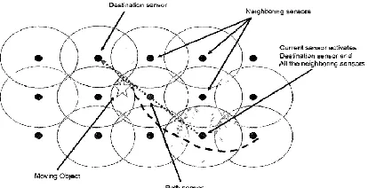
sensor-neighboring sensors-destination sensor), still expect to have a missing object running in the network. Therefore, it needs to develop a solution to find any missing object and return the network to the prediction tracking process (or as we call it the normal state), since any recovery technique will incur higher energy consumption than the normal prediction tracking technique.
Fig 1.2 The current sensor is activating all the neighboring sensors in addition to the destination sensor.
In developing three recovery mechanisms in order to determine which recovery mechanism would generate lower energy consumption compared to the others.
• Source Recovery Mechanism:
In this recovery mechanism the current sensor will activate all its neighboring sensor nodes if the object is not in its detection area and it didn't receive any ACK message from the destination sensor(s) after the passing of a certain timeout period.
• Destination Recovery Mechanism:
This recovery mechanism is similar to the previous one, except that the current sensor will activate all the neighboring sensors of the destination sensor instead of the neighboring sensors of the current sensor.
• All Neighbors Recovery Mechanism:
576 Missing Rate Analysis
The missing rate analysis only consider PTSP, since for the other basic tracking techniques (Naive, SM and CM) the missing rate is always 0%. It notice in figure 5.9 that the missing rate levels is not impacted by increase in the number of moving objects as we have expected, since the missing rate is the ratio of the missing reports to the total number of reports, therefore this ratio is not affected by the increase in the number of objects since even though it's likely that the number of missing reports will increase, this number will be matched with an increase in the number of total reports, thus the ratio remains unchanged.
Fig.1.2 Missing rate levels against the network workload.
Object Movement Speed Analysis
This experiment evaluates how the changes in the speed of a moving object could affect the energy consumed by a tracking technique. Also, since the CM is better than the SM when there is a low number of objects in the network then only use the CM for comparison purposes against PTSP.It can notice a linear growth in the energy consumption levels when the object speed also increases, which is resulted by the fact that when the object moves in a faster speed the prediction for the destination sensor will be harder and thus more recovery process is required and eventually an increase in the overall energy consumption of the network. We can notice that PTSP was outperforming CM when the object speed was below 30 m/s which is considered an excellent performance compared to the speed of the object, since tracking an object moving in a speed of 25 m/s for example is not an easy task, if energy saving is also a factor of the tracking technique.
Sampling Duration Analysis
577
doesn't depend on the sampling duration while monitoring moving objects. As for PTSP the increases in the sampling duration will increase the energy consumed by the network and also it will reduce the number of missing objects, since the current sensor is kept active longer than it used to be which means that there will be more assurance regarding the prediction of the future movement of the object. In addition, it shows that the missing rate will decrease linearly to become below 3% while the sampling duration increases, since the increase in the sampling duration results in lower number of missing reports and thus a lower missing rate.
Sampling Frequency Analysis
One of the most critical influencing factors is the sampling frequency, since this factor could affect the performance of tracking technique directly in terms of the quality of tracking and the energy consumption. It can be define that the sampling frequency as the time between reports to the base station. It's imperative for the tracking technique to execute at least one sampling per a reporting period, so that the application could receive an updated information regarding the location of the moving object(s). When the sampling frequency is increased then this would mean that the sensor node will have a better information regarding the location of the moving object and as a result will be able to accurately predict it next movement, however these increase will incur a higher energy consumption levels, since the sensor nodes will be kept active for longer time. Therefore, similar to the sampling duration the sampling frequency represent bargain between more accurate predictions or less energy consumption. So, increasing the sampling frequency may result in better predictions, however it will also mean that keeping the sensor node active for longer periods which is mainly unneeded since there are no reports to be sent. Therefore, it's recommended to tune the sampling frequency in a way that results in a better energy savings while maintaining low missing rate.
Fig.1.3 Recovery Mechanism Analysis
Recovery Mechanism Analysis
578
required the network to go for the second phase of recovery more often compared to the other recovery mechanisms. Since the second phase of recovery involves activating all the sensor nodes m the network, then it incurs more energy consumption compared to the first phase of recovery.
IV DISCUSSION
In this method developed tracking scheme explained the energy consumed by the MCU and the sensing components. Since it believed that the energy consumption contributed by the radio component should have an orthogonal affect to the simulations, The future work to study the energy consumed by the radio component. Investigating the possibility to produce more accurate sensor sequential patterns which also could be more adaptive to the changes made to the network. In addition, the effects of the moving objects' direction and speed in producing more appropriate predictions. Finally, a fault-tolerance approach will be evaluated and studied in order to mitigate the effects of nodes failure while tracking a moving object.
V .CONCLUSION
One of the key applications of the sensor networks which is widely adapted due to its huge number of implementations and usages, is the object tracking sensor network. Although, this application is known for its high demands of energy in order to perform its tasks in the best manner possible. Since the main obstacle that faces most tracking techniques in sensor networks is the fact that the sensor network suffers from a very limited power supply which in turn restricts the type of tasks to be accomplished by the sensor network. Therefore, the need to optimize the energy consumption in OTSNs is a fact must be faced. Since most the energy savings research was focusing on minimizing the energy consumed by the radio component (RF radio) in the sensor nodes by reducing the number of messages transmitted and received, Considering the energy consumed by the MCU and the sensing components in the sensor nodes which also attributed to a respectful amount of energy consumption. Therefore, developed an object tracking scheme that minimizes the time the sensor node stays in active mode (when both the MCU and the sensing component is active), thus generating a considerable amount of energy savings.
VI .FUTURE ENHANCEMENT
It introduced 3 different recovery mechanisms in regard to the neighboring sensor nodes to be activated. We have simulated our proposed tracking scheme (PTSP) along with 3 basic tracking schemes for comparison purposes. The results generated by the experiments were mainly testing the performance of PTSP and the other tracking schemes against two main metrics: (1) total energy consumed by the network during the simulation period, including the active and sleep mode energy consumption for each sensor node in the network, (2) missing rate, which represents a ratio of the missing reports to the total number of reports received by the application. Moreover, it was proven by the simulation results that PTSP outperformed all the other tracking schemes by keeping a low energy consumption levels while maintaining an acceptable level of the missing rate.
REFERENCES
[1].Sleep scheduled and tree-based clustering routing protocol for energy-efficient in wireless sensor
network Computing & Communication Technologies - Research, Innovation, and Vision for the
579
[2].A Secure Scheme Against Power Exhausting Attacks in Hierarchical Wireless Sensor Networks
IEEE Sensors Journal (Volume:15 , Issue: 6 )03 February 2015
[3]. An energy efficient routing protocol for Wireless Sensor Network.Communications (APCC),
2012 18th Asia-Pacific Conference on15-17 Oct. 2012
[4].A Novel Routing Algorithm for Energy-Efficient in Wireless Sensor Networks. Genetic and
Evolutionary Computing, 2009. WGEC '09. 3rd International Conference on 14-17 Oct. 2009 [5].Vincent S. Tseng and Kawuu W. Lin, "Energy Efficient Strategies for Object Trackingin Sensor
Networks: A Data Mining Approach", Journal of Systems and Software,Vol. 80, No. 10, pp. 1678-1698, October 2007.
[6].Y. Xu, J. Winter and W.-C. Lee, "Dual Prediction-based Reporting forObject Tracking Sensor Networks", In Proceedings of the First Annual International Con- ference on Mobile and Ubiquitous Systems: Networking and Services (MobiQuitous' 04), 2004, pp. 154-163.
[7]. S.-M. Lee, H. Cha and R. Ha, "Energy-Aware Location Error Handling for Object Tracking Applications in Wireless Sensor Networks", Computer Communication 30,2007, pp. 1443-1450. [8].Y. Xu and W.-C. Lee, "On Localized Prediction for Power Efficient
Object Tracking in Sensor Networks", In Proceedings of the 1st International Workshop on Mobile Distributed computing, Providence RI, May 2003.