http://www.sciencepublishinggroup.com/j/ijtam doi: 10.11648/j.ijtam.20190503.11
ISSN: 2575-5072 (Print); ISSN: 2575-5080 (Online)
Research on Logistics Distribution Optimization Based on
Low Carbon Constraints
Yu Xiaohao
School of Transportation, Shanghai Maritime University, Shanghai, China
Email address:
To cite this article:
Yu Xiaohao. Research on Logistics Distribution Optimization Based on Low Carbon Constraints. International Journal of Theoretical and Applied Mathematics. Vol. 5, No. 3, 2019, pp. 37-43. doi: 10.11648/j.ijtam.20190503.11
Received: August 8, 2019; Accepted: September 9, 2019; Published: September 18, 2019
Abstract: Recently, the problem of climate is becoming more and more serious and the low carbon idea is accepted by people
gradually. Meanwhile, the China’s logistic develop rapidly. Whereas, distribution as the key part, its importance is obvious to see. So, it is significant to research the distribution of logistic activity based on low-carbon with the low-carbon economy put forward. In this dissertation, the paper analyzes and summarizes the research at home and abroad. And then it distinguishes the different distribution model from economy, service and carbon. Besides, it also combines the joint distribution, the green logistic, circular logistic and reverse logistic to contrast. Based on this, the paper propose the way of calculating carbon emission and then build the math model of calculating carbon emission during distribution activity. At last, it uses the genetic algorithm as a tool to set up a experience platform. By using the platform, it researches the distribution math model based on the carbon emission. It also analyzes the result of the experience, and improve the data of the genetic algorithm.Keywords: Logistics Distribution, Carbon Emissions, Genetic Algorithm
1. Introduction
In recent years, climate issues have attracted more and more attention. According to the International Energy Agency, the logistics industry represented by the transportation industry is responsible for 23% of global CO2 emissions. The McKinsey
Global Survey (2008) shows that the world's top management is clearly aware of the significant impact of carbon emissions management on future markets in many areas, including the logistics market. Therefore, in the future environment of carbon emission limitation, the enterprise logistics business will meet the requirements of low-carbon economy more quickly, and the more obvious its logistics advantages, the more it can improve the market competitiveness of enterprises.
Based on this research on low carbon logistics at home and abroad, Tonya Boone. Vaidyanathan Jayaraman and Ram Ganeshan pointed out in their book "Sustainable Supply Chain: Models, Methods and Public Policy Applications" that sustainable supply chain development should consider logistics The emission of various CO2 in the process, and also
divide the sustainable development of the supply chain into national, urban and industrial product development [1]. Balan
Sundarakani, Robertde Souza, Mark Goh, Stephan M. Wagner, and Sushmera Manikandan's "Modeling carbon footprints across the supply chain" examine supply chain CO2 emissions,
and provide theoretical and practical experience for green supply chain management. The infinite emission model was established using the remote Lagrangian and Euler transport method finite element analysis. The results show that the carbon emissions at various stages of the supply chain may threaten the guarantee of each stage of the supply chain [2]; Ding Lianhong and Yang Mingrong analyzed the model research, relevance research and feasibility of low carbon logistics [6]; Jiang Yan and Wu Xiuguo discussed the development of low-carbon logistics from the aspects of logistics technology, logistics information system, logistics mode and laws and regulations [7].
2. Based on Low Carbon Logistics
Distribution Model Construct
2.1. Carbon Emission Measurement Method
some scholars have proposed a rough algorithm for measuring carbon emissions. This paper uses the carbon emission measurement method of the following process:
2.1.1. Determine the Type of Mobile Source
The mobile source type mainly refers to the form of transportation used in the distribution of goods, including road transportation, railway transportation, water transportation, air transportation, etc. Different types of transportation activities, that is, different types of mobile sources, have long-term carbon dioxide emissions. Great difference, so in the choice of goods delivery form should choose the appropriate form of transportation according to relevant needs, thereby reducing carbon dioxide emissions [19].
2.1.2. Determine the Calculation Method
In order to simultaneously consider the travel distance of the vehicle during the delivery process and the loading capacity of the vehicle during the delivery process. This paper
uses the following formula to calculate CO2 emissions:
CO2 Emissions = transport weight × Travel distance ×
Emission factor
Among them, CO2 emissions: carbon emissions (KG) over
a certain period of time; travel distance: vehicle travel distance (KM); emissions factor: a fuel emission coefficient.
2.1.3. Determination of Carbon Emission Factors
The carbon emissions generated by different fuels vary greatly, and the degree of combustion of the fuel is different, and the carbon emissions generated by them vary greatly. The CO2 emission factor should assume that the carbon in the fuel
is oxidized 100% after combustion or just after combustion (all vehicle fuel types). Because of the different fuel quality and composition in different places, the CO2 emission factors
will also be different, so the carbon emission factors have certain uncertainties.
Table 1. Heat generation and emission factors of different fuels.
Fuel type Heating Value [GJ/I] Emission Factor[kgCO2/GJ] Emission Factor[kgCO2/I]
Gasoline/Petrol 0.0344 69.25 2.3822
Diesel 0.0371 74.01 2.7458
propane 0.0240 62.99 1.5118
Kerosene 0.0357 71.45 2.5508
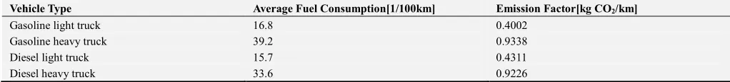
Table 2. Emission factors for different vehicle types in distance-based methods.
Vehicle Type Average Fuel Consumption[1/100km] Emission Factor[kg CO2/km]
Gasoline light truck 16.8 0.4002
Gasoline heavy truck 39.2 0.9338
Diesel light truck 15.7 0.4311
Diesel heavy truck 33.6 0.9226
2.1.4. Activity Data Selection
Different fuel types, different vehicle types, and different road types can result in different CO2 emissions. Therefore,
when calculating the CO2 emissions, a vehicle and a fuel type
are selected. Since the impact of the road on CO2 emissions
cannot be measured, the estimated value can be used or ignored.
In view of the fact that there is currently no clear calculation standard for vehicle carbon emissions, it is very difficult to calculate CO2 emissions. Referring to the IPCC mobile carbon
source carbon emissions, assuming that there is only one type of distribution vehicle in the distribution process, the calculation of the vehicle carbon emissions during the logistics distribution process can be calculated in the following order:
1) Defining the CO2 unit distance emissions of fuel;
2) Defining the total distance traveled by the delivery vehicle;
3) Defining the maximum load capacity of the vehicle; 4) Calculate the vehicle full load rate;
5) Determine the carbon emission calculation method; 6) Calculate the total carbon emissions during the logistics
distribution process.
2.2. Establishment of a Logistics Distribution Model Considering Carbon Emissions
It can be seen from the above analysis that the carbon emission impact factors in the distribution process mainly include two important factors: transportation distance and cargo load. Therefore, based on the actual situation and the factors affecting carbon emissions, the following distribution problems and mathematical models are proposed.
2.2.1. Description of the Problem
The known conditions of the problem are as follows: Set up a distribution center with goods distribution vehicles The stations are of the same type and model, and the maximum load capacity of each delivery vehicle is
( = 1,2, … , ). The maximum travel distance of each
delivery vehicle during a delivery process is ( = 1,2, … , ), the distribution center needs a total of Customer
delivery goods, among which customers . The
transportation distance to the customer is (、 =
1,2, … , ) , the total number of customers delivered for
elements Indicates the customer is in the path In the order (excluding the distribution center), use . Indicates the total weight of all customer demand for the first route, . Indicates the first route . The weight of the goods required by the customer. make . Indicates the distribution center, Indicates the carbon emission factor.
Problem: The distribution of distribution vehicles and their
transportation and distribution routes when the total carbon emissions are minimized during the distribution process.
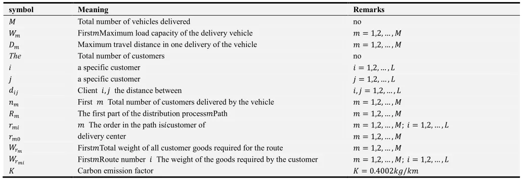
The symbols involved in this article mainly include important symbols such as vehicle, customer, cargo weight, route, etc. The meanings and value ranges of each symbol are as follows:
Table 3. Related symbol description.
symbol Meaning Remarks
Total number of vehicles delivered no
First Maximum load capacity of the delivery vehicle = 1,2, … ,
Maximum travel distance in one delivery of the vehicle = 1,2, … ,
The Total number of customers no
i a specific customer = 1,2, … ,
a specific customer = 1,2, … ,
Client , the distance between , = 1,2, … ,
First Total number of customers delivered by the vehicle = 1,2, … ,
The first part of the distribution process Path = 1,2, … ,
The order in the path is customer of = 1,2, … , ; = 1,2, … ,
delivery center = 1,2, … ,
First Total weight of all customer goods required for the route = 1,2, … ,
First Route number The weight of the goods required by the customer = 1,2, … , ; = 1,2, … ,
Carbon emission factor = 0.4002 !/
2.2.2. Model Establishment
The objective function is to measure the total carbon emissions generated during the entire distribution process. It is easy to know according to the calculation method in Section 1.1:
Since the vehicle load has not been clearly related to its carbon emissions so far, this article orders:
Therefore, in summary, the following objective functions and constraints are easily obtained:
: $ = %{ × %[ ( )*) × (1 + − )] + × . / 0× 1 ! ( )}
3
45 6
45
= %{ × %[ ( )*) × (1 + − )] + . / 0× 1 ! ( )}
3
45 6
45
= × ∑645{∑ [345 ( )*) × (1 +8/ 898/ )] + . / 0× 1 ! ( )} (1)
:. ; ≤ (2)
∑3 45 = (3)
∑345 ( )*) + . × 1 ! ( ) ≤ (4)
0 ≤ ≤ (5)
∑6 45 = (6)
= { | ∈ {1,2, … , }, = 1,2, … , } (7)
5∩ @= ∅, ∀ 5≠ @ (8)
1 ! ( ) = D1 1 ≤ 0 E;ℎG 1 (9)
0 ≤ (10)
0 ≤ (11)
In the above model:
Equation (1) is the objective function, which requires minimum carbon emissions generated during the distribution process;
Equation (2) ensures that the sum of the cargo requirements of each customer on each distribution route does not exceed the load capacity of the delivery vehicle;
Equation (3) ensures that the sum of the cargo demand of each customer on each delivery route is equal to the amount of cargo transported by the delivery vehicle;
Equation (4) ensures that the length of each delivery path does not exceed the maximum distance traveled by the delivery vehicle at one time;
Equation (5) ensures that the number of customers per path does not exceed the total number of customers;
each route;
Equation (8) ensures that each customer can only be delivered by one delivery vehicle;
Equation (9) guarantees that when the number of customers serving the mth car is ≥1, it means that the car has participated in the delivery, then 1 ! ( ) =1; when the number of customers serving the mth car is <1, it means that the car is not used, so take 1 ! ( ) =0;
Equation (10) guarantees a non-negative requirement for the distance traveled by the vehicle;
Equation (11) guarantees non-negative requirements for customer demand for goods.
3. Genetic Algorithm Design
3.1. Determination of Algorithm Strategy
For the above problem model, the coding method, fitness assessment method and genetic operator should be comprehensively analyzed to design the genetic algorithm. The specific algorithm strategy is as follows:
3.1.1. Coding Method
The coding method directly arranged by the customer is adopted, that is, the customer randomly arranges according to the serial number without repetition, and the arrangement constituted by the customer constitutes a solution to the problem, that is, a distribution method is generated. Assume that there are 3 vehicles that need to deliver goods to 5 customers, so that the customer's arrangement is 32541. The delivery route can be obtained as follows: First, customer 3 is the first customer of the first vehicle service, combined with the first vehicle. The maximum load capacity and the maximum travel distance determine whether the customer 3 satisfies the condition. If it is satisfied, the customer who takes 2 as the second service also judges whether the condition is satisfied according to the maximum load capacity and the maximum travel distance of the vehicle, and if so, if it is not satisfied, try to find the next customer at a time. If it is not satisfied, return to the distribution center and serve the other customers by the next vehicle. With this representation method, it is possible to obtain a delivery route scheme in which the delivery scheme is smaller than the total number of vehicles. In addition, if all customers cannot be serviced, that is, the delivery vehicle cannot pass through all the customers, the solution is an infeasible solution.
3.1.2. Fitness Function
Set the objective function value of the distribution path scheme corresponding to a solutionH, the number of infeasible paths is . The penalty weight for the infeasible path isIJ, the evaluation value of the solution K = H + × IJ. According to the requirements of the fitness function, the individual's fitness f can be calculated by the reciprocal of the evaluation value, namely:
L =1K =H + × IJ1
The above formula can be used as a function of calculating the fitness of an individual.
3.1.3. Selection Strategy
Use the selection strategy that combines the best individual and the gambling wheel selection. The method of operation is as follows: each individual in the group is arranged according to the order of fitness, and the individual ranked first has the greatest fitness, and directly copies it into the next generation and ranks first. Other individuals in the next generation group need to be produced by contemporary groups through the gambling wheel selection method.
3.1.4. Crossover Operator
The OX-like crossover method is adopted. In actual operations, the crossover operation is probabilityIMoccurring.
3.1.5. Mutation Operator
Multiple conversion methods are used. In the case of normal operation, the mutation operation is based on probability.I Occurred, once the mutation operation occurs, a random method is used to generate the number of exchanges. N, for the genes of individuals who need to undergo mutation operationsNSecond swap.
3.1.6. Termination Criteria
Use the termination criteria of the specified evolutionary algebra, that is, the criteria for terminating the program after the number of evolutions is set.
3.2. Genetic Algorithm Structure
According to the above genetic algorithm strategy, the following algorithm structure can be obtained:
{
Enter the corresponding known conditions in the distribution problem in the model;
Enter relevant operating parameters, such as group size O, terminating evolutionary algebra P Cross probability IM Variation probability I , the number of gene transpositions when performing the mutation operation N, the penalty weight for the infeasible pathIJWait;
Randomly generate an initial group I(0) Current evolution algebra ; = 0;
Calculation I(0) . Fitness function value for each individual in;
While (t< Evolutionary Termination Algebra T) do {
Copy the individuals with the highest fitness in the current generation and insert them into the new group P(t+1);
Calculating the selection probability Pi of each individual in the group according to the gambling wheel selection strategy and the fitness of the individual generation;
For (k=0; k<N; k=k+2) {
Select two parents from the group P(t) according to the selection probability Pi;
r=random [0, 1];
two individuals with the OX-like method and inserts the generated two generations into the new population P(t+1);
else {
r=random [0, 1];
If (r ≤ mutation probability Pm), the parent individual 1 is mutated, and then the individual generated after the mutation is inserted into the new group P(t+1);
Else copies the parent individual 1 and then inserts it into the new group P(t+1);
r=random [0, 1];
If (r ≤ mutation probability Pm), the parent individual 2 is subjected to mutation operation, and then the individual generated after the mutation is inserted into the new group P(t+1);
Else copies the parent individual 2 and then inserts it into the new group P(t+1);
} }
Calculating the fitness function values of each individual in the P(t+1) population;
t=t+1; }
Output target function value distribution plan, use vehicle and other related values;
}
4. Experimental Simulation Results and
Analysis
4.1. Simulation Platform
This article uses the simulation platform is the Visual Studio 2010 development environment that Microsoft quits,
and is developed using the C# programming language. By using the C# windows form application to write the simulation platform interface, the background operation program is designed according to the genetic algorithm strategy of Chapter 3.
The simulation platform has important information such as carbon emissions, vehicle plan, vehicle travel route, and other algorithm information such as initial population, final population, and program running time. By clicking on the “Run” interface, the platform will run once and generate a feasible solution to get a distribution plan and its carbon emissions.
From the above running results interface graph, it is easy to know the information directly related to solving the problem such as carbon emissions, vehicle number, vehicle route and vehicle plan. In addition, we can also obtain some algorithm information, such as the initial population of the algorithm, fitness and other related information. This article focuses on the analysis of model results, and the relevant content of the algorithm is not described in detail.
4.2. Study Description
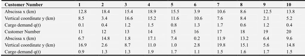
There is a distribution center and 20 customers in a certain area. The demand for goods of each customer is less than 2t. There are 5 distribution vehicles in the distribution center. The maximum cargo load of each vehicle is 8t, and each vehicle is in the vehicle. The maximum travel distance during a delivery process is 50km. The location coordinates of the distribution center and the location coordinates of the 20 customers and the demand for the goods are randomly generated by using a computer program, and the position coordinates of the distribution center are (14.5km, 13.0km), the location coordinates of 20 customers and the required cargo demand are shown in the table below.
Table 4. 20 customer coordinates and their cargo demand.
Customer Number 1 2 3 4 5 6 7 8 9 10
Abscissa x (km) 12.8 18.4 15.4 18.9 15.5 3.9 10.6 8.6 12.5 13.8
Vertical coordinate y (km) 8.5 3.4 16.6 15.2 11.6 10.6 7.6 8.4 2.1 5.2
Cargo demand q(t) 0.1 0.4 1.2 1.5 0.8 1.3 1.7 0.6 1.2 0.4
Customer Number 11 12 13 14 15 16 17 18 19 20
Abscissa x (km) 6.7 14.8 1.8 17.1 7.4 0.2 11.9 13.2 6.4 9.6
Vertical coordinate y (km) 16.9 2.6 8.7 11.0 1.0 2.8 19.8 15.1 5.6 14.8
Cargo demand q(t) 0.9 1.3 1.3 1.9 1.7 1.1 1.5 1.6 1.7 1.5
Requirements: Through the reasonable and effective arrangement of the delivery vehicles and delivery routes, the carbon emissions generated during the entire distribution process are the lowest.
In this problem, there are 5 distribution vehicles in the distribution center, and each vehicle has certain conditions for the load capacity and driving distance. In addition, there are 20 customers, each customer's position coordinates are random, and the cargo demand is not the same, there is no regularity. Therefore, there are many vehicle delivery and route selection schemes for distributing goods from the distribution center to each customer, and the scale is large. If the exhaustive method
is used to solve the problem, it is difficult to find the optimal solution. Therefore, the author uses genetic algorithm to solve the problem.
4.3. Simulation Results and Analysis
In this genetic algorithm, select the population size O = 40 Evolutionary termination algebra P = 400 Cross probability IM = 0.9. Variation probability I = 0.9, mutation is the number of gene transpositions N = 5. Punitive weight of the infeasible path IJ = 300 . The final result of the program is shown in the following figure:
of vehicles used in the distribution process, the route of the vehicle, and the amount of carbon emissions during the distribution process are easily known.
Run the program 10 times and get the calculation results as shown in the following table:
Table 5. The algorithm raw data is run 10 times the result statistics table (unit: kg).
Calculation order 1 2 3 4 5 6 7 8 9 10 average
carbon emission 77.95 77.63 72.24 69.77 75.11 75.15 73.39 77.36 71.03 77.23 74.689
It is easy to know from the above results that the solutions obtained by the genetic algorithm are suboptimal solutions, and the best quality in the suboptimal solution is 69.77kg. The worst quality is 77.95kg.
1. Set the evolution termination algebra to P = 800 Generation, other relevant data is unchanged, the program is run 10 times, the results are as follows:
Table 6. Let T=800 run 10 times result statistics table (unit: kg).
Calculation order 1 2 3 4 5 6 7 8 9 10 average
carbon emission 72.63 70.70 71.99 72.59 72.76 70.25 71.50 72.67 68.10 72.59 71.578
From the above results, the termination algebra is set to P = 800. The best quality of the suboptimal solution is 68.10kg, and the worst quality is 72.67kg. Compared with the initial results, it is easy to find that when the evolutionary algebra increases, the quality of the solution is improved.
2. Set the group size to O = 100, other relevant data is unchanged, the program is run 10 times, the results are as follows:
Table 7. Make O = 100 Run 10 times result statistics table (unit: kg).
Calculation order 1 2 3 4 5 6 7 8 9 10 average
carbon emission 74.40 75.99 70.16 75.30 70.48 74.33 67.99 71.71 75.79 71.71 72.786
It is easy to know from the above results that the group size is set to O = 100. When the suboptimal solution quality is 67.99kg, the worst quality value is 75.99kg. Compared with the initial results, it is easy to find that when the population
size increases, the quality of the solution is improved. 3. Set the crossover probability to IM = 0.1, other relevant data unchanged, the program runs 10 times, the results are as follows:
Table 8. Make IM = 0.1 Run 10 times result statistics table (unit: kg).
Calculation order 1 2 3 4 5 6 7 8 9 10 average
carbon emission 80.83 92.85 87.36 89.60 79.49 89.71 85.47 84.17 86.96 87.52 86.396
It is easy to know from the above results that the crossover probability is set to IM = 0.1. When the suboptimal solution quality is 79.49kg, the worst quality value is 92.85kg. Compared with the initial results, it is easy to find that when the crossover probability decreases, the quality of the solution
is reduced.
4. Set the mutation probability to I = 0.1, other relevant data is unchanged, the program is run 10 times, the results are as follows:
Table 9. Make I = 0.1 Run 10 times result statistics table (unit: kg).
Calculation order 1 2 3 4 5 6 7 8 9 10 average
carbon emission 76.44 69.99 72.72 71.49 76.26 75.51 72.77 69.71 72.43 73.82 73.114
It is easy to know from the above results that the mutation probability is set to I = 0.1. When the suboptimal solution quality is 69.71kg, the worst quality value is 76.44kg. Compared with the initial results, it is easy to find that when the mutation probability decreases, the quality of the solution does not change much.
Therefore, through the above comparison, the relevant
algorithm data in the genetic algorithm is set as follows: group size O = 100. Evolutionary termination algebra P = 800 Cross probability IM = 0.1. Variation probability I = 0.9, mutation is the number of gene transpositions N = 5. Punitive weight of the infeasible path IJ = 300 . Run the program 10 times at random to get the results as follows:
Table 10. Algorithm optimization data run 10 times result statistics table (unit: kg).
Calculation order 1 2 3 4 5 6 7 8 9 10 average
carbon emission 66.65 67.55 68.57 67.51 68.31 67.66 69.11 68.05 68.23 69.10 68.074
It is easy to know from the above results that the best value of the suboptimal solution is 66.65 kg, and the worst quality value is 69.11 kg. Compared with the initial results, it is easy
the objective function. The running result is as shown in the figure:
As can be seen from the above figure, the optimal delivery plan is:
Use 4 cars to deliver, the specific delivery route is as follows:
(1) Vehicle 1 route: 0-1-7-16-13-6-11-20-0; (2) Vehicle 2 route: 0-12-2-9-15-19-8-0; (3) Vehicle 3 route: 0-18-17-10-3-4-0; (4) Vehicle 4 route: 0-14-5-0.
The total carbon emissions generated are: 66.65kg
5. Conclusion
The author collects literature on the quantitative calculation of carbon emissions, analyzes and summarizes them, and identifies the factors that calculate carbon emissions as two factors: distance and load. Taking carbon emission as the standard of vehicle routing in the process of logistics and distribution, by analyzing the relevant influencing factors of carbon emissions, a mathematical model of logistics distribution with the minimum carbon emission as the objective function is established.
Then the genetic algorithm of the mathematical model of logistics and distribution of carbon emissions is considered, and the algorithm is designed. It is concluded that the reasonable optimization of the vehicle route in the distribution process can greatly reduce the carbon emission of the distribution process. It is of great significance to both the company and the environment.
References
[1] Tonya Boone•Vaidyanathan Jayaraman, Ram Ganeshan. Sustainable Supply Chains: Models, Methods, and Public Policy Implications [M]. Springer New York Dordrecht Heidelberg London.
[2] M. Soysal n, J. M. Bloemhof-Ruwaard, J. G. A. J. vander Vorst. Modelling food logistics networks with emission considerations: The case of an international beef supply chain [J]. Int. J. Production Economics, Accepted 10 December 2013.
[3] Tsai Chi Kuo, Hsiao Min Chen, Chia Yi Liu, Jui-Che Tu, and Tzu-Chang Yeh. Applying Multi-Objective Planning in Low-Carbon Product Design [J]. INTERNATIONAL JOURNAL OF PRECISION ENGINEERING AND MANUFACTURING Vol. 15, No. 2, pp. 241-249.
[4] Ki-Hoon Lee. Carbon accounting for supply chain management in the automobile industry [J]. Journal of Cleaner Production 36 (2012) 83e93.
[5] Zheng Kai, Zhu Xi, Yan Yihong. Low Carbon Logistics [M]. Beijing: Beijing Jiaotong University Press, 2011.8.
[6] Ding Lianhong, Yang Mingrong. Review of Low Carbon Logistics Research [J]. Logistics Technology. ISSN. 1005-152X. 2013.03.005.
[7] Jiang Yan, Wu Xiuguo. Analysis of low carbon logistics [A]. Economy and Management. 1003-3890 (2011) 07-0079-05. [8] Yang Yuwei. Summary of research on low carbon logistics at
home and abroad [J]. Logistics Engineering and Management. ISSN. 1674-4993.2011.03.001.
[9] Zhang Jinying, Shi Meizhen. Analysis of the “four in one” low carbon logistics talent training model [J]. Logistics Technology. ISSN. 1005-152X. 2010.15.050.
[10] Li Yang, Wei Heng. Problems and countermeasures of low carbon logistics of agricultural products in China [A]. Journal of Harbin University of Commerce. 167-7112(2011)06-0019-05.
[11] Lu Duan, Tang Limin. Research on System Dynamics Model of Low Carbon Linkage Development in Manufacturing Industry and Logistics Industry. Logistics Engineering and Management [J]. ISSN. 1674-4993.2013.03.034.
[12] Li Xiaoxiang, Lu Xiaocheng. Research on China's low carbon logistics financial support model [A]. China's circulation economy. 1007-8266 (2010)02-0027-04.
[13] Cui Yuying, Luo Junhao, Ji Jianhua. Research on logistics network design under carbon tax and carbon trading environment [J]. Science and Technology Management Research. ISSN 1000-7695.2012.22.051.
[14] Logistics [M]. Beijing: Higher Education Press, 2009. 2. [15] Song Hua, Yu Yan. Modern Logistics Management [M].
Beijing: China Renmin University Press, 2012. 7.
[16] Yu Baoqin, Wu Jinjin. Modern Logistics Distribution Management [M]. Beijing: Peking University Press, 2009.8 [17] Hartmut Zadek, Robert Schulz. Methods for the Calculation of
CO2 Emissions in Logistics Activities [J]. W. Dangelmaier et
al. (Eds.): IHNS 2010, LNBIP 46, pp. 263–268, 2010. [18] Ki-Hoon Lee. Integrating carbon footprint into supply chain
management: the case of Hyundai Motor Company (HMC) in the automobile industry [J]. Journal of Cleaner Production 19 (2011) 1216e1223.
[19] Song Yu. Research on low carbon effect of building circulation logistics system [D]. Beijing Jiaotong University, July 2011.