On Technique for Generating Pareto Optimal Solutions of Multi-objective Linear Programming Problems

http://www.sciencepublishinggroup.com/j/sjams doi: 10.11648/j.sjams.20190702.12

ISSN: 2376-9491 (Print); ISSN: 2376-9513 (Online)

On Technique for Generating Pareto Optimal Solutions of

Multi-objective Linear Programming Problems

Effanga Effanga Okon

1

, Edwin Frank Nsien

2

1

Department of Statistics, University of Calabar, Calabar, Cross River State, Nigeria

2_{Department of Mathematics/Statistics, University of Uyo, Uyo, Akwa Ibom State, Nigeria}

Email address:

To cite this article:

Effanga Effanga Okon, Edwin Frank Nsie. On Technique for Generating Pareto Optimal Solutions of Multi-Objective Linear Programming Problems. Science Journal of Applied Mathematics and Statistics. Vol. 7, No. 2, 2019, pp. 15-20. doi: 10.11648/j.sjams.20190702.12

Received: April 1, 2019; Accepted: May 23, 2019; Published: June 10, 2019

Abstract:

Subjective selection of weights in method of combining objective functions in a multi – objective programming problem may favour some objective functions and thus suppressing the impact of others in the overall analysis of the system. It may not be possible to generate all possible Pareto optimal solution as required in some cases. In this paper we develop a technique for selecting weights for converting a multi-objective linear programming problem into a single objective linear programming problem. The weights selected by our technique do not require interaction with the decision makers as is commonly the case. Also, we develop a technique to generate all possible Pareto optimal solutions in a multi-objective linear programming problem. Our technique is illustrated with two and three objective function problems.

Keywords:

Multi-objective, Single Objective, Linear Programming, Pareto Optimal Solution, Weight, Non-inferior Solution

1. Introduction

There is increasing interest in research in the area of multi-objective programming. [1] presents an alternative method based on fuzzy programming for solving multi-objective linear bi-level multi-follower programming problem in which there is no sharing of information among followers; a multi-objective programming model for selecting third – party logistics companies and suppliers in a closed-looped supply chain was proposed in [2-3] proposed a fuzzy robust programming approach to multi-objective portfolio optimization problem under uncertainty and lot more.

A feasible solution to a multi-objective linear programming problem is considered to be optimal if it is better than any other feasible solution for all linear programming problems that constitute the multi-objective programming problem. But such an optimal solution to a multi-objective programming problem does not always exist and we must compromise in our analysis of the problem. We desire to obtain variety of good, but not necessarily optimal solutions.

A good but, not necessarily optimal solution to a multi-objective linear programming problem is known as efficient

or non-inferior or Pareto optimal solution. In other words, a solution to a multi-objective linear programming problem is said to be efficient if it is not possible to improve some objective function values at expense of others. Such solutions are infinitely many and so interest is always on generating some of them.

Generally, solution methods of multi-objective linear programming problems may be classified into three groups, viz:priori, interactive, and posterior methods [4]. In a priori method, the decision maker states his preferences before selecting weights to combine several objectives function to form single objective function. The pitfall of this method is that it is not easy for the decision maker to accurately quantify his preferences prior to optimization [5].

process. For detail interactive methods the reader is referred to [6-13]

In the posterior method, all the solutions are generated and presented before the decision maker who will either accept or reject it [14]. This method has advantage over the other two in the sense that the decision maker may or may not be present while the optimization procedure is ongoing and no potential optimal solution will be left out. A simplex based approach known as non-dominance subroutine to determine all non-inferior basic solutions to multi-objective programming problems was developed in [15]. The problems with the simplex based approach are that, it is too lengthy and requires a lot of bookkeeping.

In most cases, method of converting multi-objective linear programming problem into a single objective linear programming problem is often used because the solution procedure is already known. Subjective selection of weights in method of combining objective functions may favour some objective functions and thus suppressing the impact of others in the overall analysis of the system. It may not be possible to generate all possible Pareto optimal solution as required in some cases.

In this paper we present a technique for weights determination that does not involve interaction with the decision maker while the optimization process is ongoing, and also the procedure for the generation of all Pareto optimal solutions is presented.

2. Methodology

2.1. General Multi-objective Linear Programming Problem

The general Multi-objective linear programming problem is stated as

P1

n

1 1j j j 1

n 2 2j j

j 1

n p pj j

j 1

max z c x

max z c x

max z c x

=

=

=

=

=

=

∑

∑

∑

⋮

Subject to:

n

ij j i j 1

a x b , i 1, 2, . . . , m

=

≤ =

∑

j

x ≥ 0, j = 1, 2, . . . , n

2.2. Weights Determination

Selecting adequate weights in multi-objective linear programming problem is not always easy. One method of

doing this is through the use of utility function. If utility function U(x) is known, one can select weight wk through

k k _p

k

k 1

u (x)

w , k 1, 2, . . . , p

u (x) =

= =

∑

(1)

[16] proposed the following utility functions

p

k k 1

u(x) z

=

=

∏

(2)

p 2 k k 1

u(x) z

=

=

∑

(3)

p k k 1

z

u(x) = e

∑

= (4)

p

k k 1

u(x) log z

=

=

∏

(5)

Theorem 1:

Let xk, k = 1, 2,..., p be optimal solutions to p single objective linear programming problems LP1, LP2,..., LPp, respectively. Let (z , z , ₁k k₂ ⋯ , z )k_{p , k = 1, 2,..., p be the}

corresponding points in the objective function space. Then the appropriate weights wk, k = 1, 2,..., p to be attached to Zk, k =1, 2,..., p that will give additional Pareto optimal solution are given by

k _p

k 1

1k 1k

C

w , k 1, 2, . . . , p

C =

= =

∑

(6)

Proof:

First, we consider a two objective functions case (i.e p = 2). Let x1 and x2 be the optimal solutions to single objective linear programming problems LP1 and LP2, respectively. Let

1 1 1 2

(z , z ) and (z , z )₁2 2₂ be the corresponding points in the objective function space. Then the line segment joining these points is given as

2 1 2 2

1 2 2 1

1 1

z

z z

z

z z z −

= +

− (7)

Now adding the coefficients of Z1 and Z2 in equation (7), we obtain

2 1 2 1 2 1

2 2 2 2 1 1

2 1 2 1

1 1 1 1

z (z ) (z )

1

z z

z z z

z z

− _{+ =} − + −

− −

2 1 2 1

2 2 1 1

2 1 2 1 2 1 2 1

2 2 1 1 2 2 1 1

z z

1

(z ) (z ) (z ) (z )

z z

z z z z

− ₊ − ₌

− + − − + − (8)

Clearly,

2 1 2 2

1 _{2 1 2 1}

2 2 1 1

z

(z ) (z )

z w z z − = − + − 2 1 1 1

2 2 1 2 1

2 2 1 1

z w

(z ) (z )

z

z z

− =

− + −

To ensure that w1 and w2 are nonnegative, we set

2 1

2 2

1 _{2 1 2 1}

2 2 1 1

11 11 12 z _C C z z z w C z z − = = +

− + − (9)

2 1 1 1

2 _{2 1 2 1}

2 2 1 1

12 11 12 z C C z z z w C z z − = = +

− + − (10)

Where C1k, k =1, 2 are the cofactors of the elements in row 1 of the matrix

1 1

1 1 2 2 2 1 2 1 1 1 2 2

z z z z

Z

z z z z

 _{− −} 

 

=_{ }

− −

 

Now, for p =3, let x1, x2 and x3 be optimal solutions to the three single objective linear programming problems LP1, LP2 and LP3, respectively.

Let (z , z , z )1₁ 1₂ 1₃ , (z , z , z )₁2 2₂ 2₃ and (z , z , z )₁3 3₂ 3₃ be the corresponding points in the objective function space. Then the plane passing through these points is given by the equation

1 1 1

1 1 2 2 3 3 2 1 2 1 2 1 1 1 2 2 3 3 3 1 3 1 3 1 1 1 2 2 3 3

z z z z z z

z z z z z z 0

z z z z z z

− − −

− − − =

− − −

(11)

Evaluating the determinant in equation (11), we obtain the equation of the plane as

11 1 12 2 13 3

c z + c z + c z = d (12)

Where

1 1 1

11 1 12 2 13 3

d = c z + c z + c z

and C1k, k =1, 2, 3 are the cofactors of the elements in row 1 of the matrix

1 1 1

1 1 2 2 3 3

2 1 2 1 2 1

1 1 2 2 3 3

3 1 3 1 3 1

1 1 2 2 3 3

z z z z z z

Z z z z z z z

z z z z z z

 _{− − −}      = − − −    _{− − −}   

Dividing equation (10) through by (c11 + c12 + c13), we

obtain

1 1 w2 2 w3 3 d

w z + z + z = ′ (13)

Where

1k

11 12 13

c

k

w

c c c

=

+ + and 11 12 13

d d

c c c

′ =

+ +

To ensure that wk is nonnegative, we set

1k

11 12 13

c

k

w

c c c

=

+ + , k = 1, 2, 3

The above results can easily be extended to p > 3 objective functions problem as follows:

k _p

k 1

1k 1k

C

w , k 1, 2, . . . , p

C =

= =

∑

2.3. Finding Additional Pareto Optimal Solution in a Two – Objective Problem

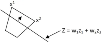
In order to find additional Pareto optimal solution (if one exists) in a two – objective linear programming problem, we could try to move the line segment joining x1 and x2 in the direction of arrow in figure 1. Algebraically, this means solving the single objective function problem P3.

P3: max{ z = w1 1z + w2 2z }

Subject to:

n

ij j i j 1

a x b , i 1, 2, . . . , m =

≤ =

∑

j

x ≥ 0, j = 1, 2, . . . , n

Lemma 1:

The set of non-inferior points is connected [17] Lemma 2:

If x1 and x2 are two adjacent non-inferior points, then their convex combination is non-inferior [17]

Lemma 3:

If x1 and x2 are two non adjacent non-inferior points, then there exists at least one non – inferior point in the range (x1, x2) [17]

Theorem 2:

If x1 and x2 are nonadjacent Pareto optimal solutions, then the solution of problem P3 is an additional Pareto optimal solution of problem P1.

Proof:

optimal solution of P3 is a Pareto optimal solution x3 of problem P1. Figure 1 illustrates theorem 2.

Figure 1. Illustration of Theorem 2

Theorem 3:

If x1 and x2 are adjacent Pareto optimal solutions, then the optimal solutions of problem P3 will be on the line segment joining x1 and x2 in which case x1 and x2 are the only Pareto optimal solution.

Proof:

Since Pareto optimal solutions are connected and if x1 and x2 are adjacent there does not exists any Pareto optimal solution between them; hence solutions of problem P3 are x1 and x2. Figure 2 illustrates theorem 3.

Figure 2. Illustration of Theorem 3.

Remark 1:

Supposing an additional Pareto optimal solution x3 has been found using known solutions x1 and x2, one can investigate the existence of another Pareto optimal solution by using known solutions x1 and x3 as well as x2 and x3. We can continue this process until all the Pareto optimal solutions are found.

Remark 2:

In order to find an additional Pareto optimal solution (if one exists) given p Pareto optimal solutions xk, k = 1, 2,..., p in a p – objective linear programming problem, we solve the scalar problem P4.

P4:

p

k k k 1

max{ z w z }

=

=

∑

Subject to:

n

ij j i j 1

a x b , i 1, 2, . . . , m

=

≤ =

∑

j

x ≥ 0, j = 1, 2, . . . , n

Remark 3:

If the solution xp+1 of P4, is an additional Pareto optimal solution to problem P1, then one can investigate the existence of another Pareto optimal solution by replacing one of the previous p Pareto optimal solutions with xp+1 and solving problem P4 again. The process continues until all the Pareto

optimal solutions are found.

Example 1: (illustrating two objective functions problem)

LP1 Maximize Z1 = -8x1 + x2

LP2 Maximize Z2 = 10x1 + 3x2

Subject to:

5x1 + 3x2 ≤ 15

-4x1 + 2x2 ≤ 8

x1 ≤ 2

x2 ≤ 4.2

x1, x2 ≥ 0

First, we solve single objective function problems LP1 and LP2 to obtain two extreme Pareto optimal solutions shown in the Table 1.

Table 1. Combing objective functions of LP1 and LP2 using (x1_{, x}2_).

X = (x1, x2) (Z1, Z2) (w1, w2) Z = w1Z1 + w2Z2

x1 _{= (0, 4) (4, 12)}

(0.42, 0.58) Z = 2.44x1 + 2.16x2

x2 _{= (2, 1.7) (-14.3, 25.1)}

We then solve the following scalar problem

Maximize Z = 2.44x1 + 2.16x2

Subject to:

5x1 + 3x2 ≤ 15

-4x1 + 2x2 ≤ 8

x1 ≤ 2

x2 ≤ 4.2

x1, x2 ≥ 0

The solution of the scalar problem is x3 = (0.48, 4.2) which is additional Pareto optimal solution. Now, we investigate the existence of another Pareto optimal solution by considering (x1, x3) and (x2, x3). Using (x1, x3) we obtain the results in Table 2.

Table 2. Combing objective functions of LP1 and LP2 using (x1_{, x}3_).

X = (x1, x2) (Z1, Z2) (w1, w2) Z = w1Z1 + w2Z2

x1 = (0, 4) (4, 12)

(0.6, 0.4) Z = -0.8x1 + 1.8x2

x3 _{= (0.48, 4.2) (0.36, 17.4)} The scalar problem is

Maximize Z = -0.8x1 + 1.8x2

Subject to:

5x1 + 3x2 ≤ 15

-4x1 + 2x2 ≤ 8

x2 ≤ 4.2

x1, x2 ≥ 0

The solution of the scalar problem is x4 = (0.1, 4.2) which

is additional Pareto optimal solution. Now, we investigate the existence of another Pareto optimal solution by considering (x2, x3).

Table 3. Combing objective functions of LP1 and LP2 using (x2_{, x}3_).

X = (x1, x2) (Z1, Z2) (w1, w2) Z = w1Z1 + w2Z2

x2 _{= (2, 1.7) (-14.3, 25.1)}

(0.34, 0.66) Z = 3.88x1 + 2.32x2

x3 _{= (0.48, 4.2) (0.36, 17.4)} The scalar problem is

Maximize Z = 3.88x1 + 2.32x2

Subject to:

5x1 + 3x2 ≤ 15

-4x1 + 2x2 ≤ 8

x1 ≤ 2

x2 ≤ 4.2

x1, x2 ≥ 0

The solution of the scalar problem is x5 = (2, 1.7) which is the same as x2. There is no new Pareto optimal solution is this range.

Returning to the using (x1, x4) and (x3, x4) we found that there does not exist Pareto optimal solutions. So the complete Pareto optimal solutions are x1 = (0, 4), x2 = (2, 1.7), x3 = (0.48, 4.2) and x4 = (0.1, 4.2).

Example 2 (Illustrating three objective functions problem):

LP1 Maximize Z1 = -8x1 + x2

LP2 Maximize Z2 = 10x1 + 3x2

LP3 Maximize Z3 = -0.8x1 + 1.8x2

Subject to:

5x1 + 3x2 ≤ 15

-4x1 + 2x2 ≤ 8

x1 ≤ 2

x2 ≤ 4.2

x1, x2 ≥ 0

Solving the three single objective function problems LP1, LP2 and LP3 we obtain the results shown in Table 4.

Table 4. Combing objective functions of LP1 and LP2 using (x1, x2, x3).

X = (x1, x2) (z1, z2, z3) (w1, w2, w3) Z = w1z1 + w2z2 + w3z3

x1 _{= (0, 4) (4, 12, 7.2)}

(0.241, 0.235, 0.525) Z = 0.002x1 + 8.236x2

x2 _{= (2, 1.7) (-14.3, 25.1, 4.66)}

x3 _{= (0.1, 4.2) (3.4, 13.6, 7.64)}

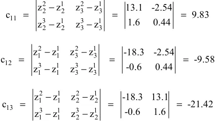
We compute the cofactors c1k from the determinant in equation (9) thus:

2 1 2 1 2 2 3 3 11 _{3 1 3 1} 2 2 3 3

z z z z 13.1 -2.54

c 9.83

1.6 0.44

z z z z

− −

= = =

− −

2 1 2 1 1 1 3 3 12 _{3 1 3 1} 1 1 3 3

z z z z -18.3 -2.54

c -9.58

-0.6 0.44

z z z z

− −

= = =

− −

2 1 2 1 1 1 2 2 13 _{3 1 3 1} 1 1 2 2

z z z z -18.3 13.1

c -21.42

-0.6 1.6

z z z z

− −

= = =

− −

Then from equation (8) we obtain the weights: w1 = 0.241, w2 = 0.235, w3 = 0.525

The associated scalar problem is

Maximize Z = 0.002x1 + 8.236x2

Subject to:

5x1 + 3x2 ≤ 15

-4x1 + 2x2 ≤ 8

x1 ≤ 2

x2 ≤ 4.2

x1, x2 ≥ 0

The solution of the scalar problem is x4 = (0.48, 4.2). We now investigate the existence of additional Pareto optimal solution by considering the solutions (x1, x2, x4), (x1, x3, x4) and (x2, x3, x4). None of these give additional solution.

3. Conclusion

solved. Even though simplex method can find all basic Pareto optimal solutions like ours it is too lengthy and requires a lot of bookkeeping. Our method is simple and easy to understand compared to the simplex method and other existing methods.

References

[1] Lachhwanni, K. C. (2018): On Solving multi-objective linear bi-level multi-follower programming. International Journal of Operations Research. Inderscience Online, Vol. 31, Issue 4. [2] Omrani, H; Hushyar, H; Zolmabadi, S. M; Asi, A. J. (2018): A

multi-objective programming model for selecting third – party logistics companies and suppliers in a closed-looped supply chain. International Journal of Operations Research. Inderscience Online, Vol. 30, Issue 4.

[3] Khanjarpanah, H and Pishvaee, M. S (2017): A fuzzy robust programming approach to multi-objective portfolio optimization problem under uncertainty. International Journal of Operations Research. Inderscience Online, Vol. 12, Issue 1. [4] Hwang, C. L. and Masud, A. S. (1979). Multiple objectives

decision making: Methods and Applications. Springer. [5] Mavrotas, G. (2007). Generation of efficient solutions in

multi-objective mathematical programming problems using games. Effective implementation of the e – constraint method. Lecturer, Laboratory of Industrial and Economics. School of Chemical Engineering. National technical University of Athens.

[6] Steuer, R. E. (1977). An interactive multi-objective linear programming procedure. TIMS Stud. Management Science, 6, 225–239.

[7] Sprong, J. (1981). Interactive Multiple Goal Programming. Nijhoff, Leiden, The Netherlands. 211pp.

[8] Korhonen, P. & Laakso, J. (1986). A visual interactive method for solving the multi-criteria problem. European Journal of Operations Research, 24, 277–287.

[9] Gardiner, L. R. & Steuer, R. E. (1994). Unified interactive multi-objective programming. European Journal of Operations Research, 74, 391–406.

[10] Stewart, J. (1999). Concepts of interactive programming. Advances in MCDM models, Algorithms. Theory and Applications, Kluwer Academic Publishers, Boston. 299 pp. [11] Branke, J; Deb, K; Miettinen, K. & Slowinsk (2008).

Mult-objective optimization: Interactive and Evolutionary Approaches. Springer-verlag Bellin Heidenlbetg. 481 pp. [12] Sadrabadi, M. R. & Sadjadi, S. J. (2009). A new interactive

method to solve multi- objective linear programming problems. J. Software Engineering & Application, 2, 23 –247. [13] De, P. K. & Yadav, B. (2011). An algorithm for obtaining

optimal compromise solution of a mult-objective fuzzy linear programming problem. International Journal of Computer Application, 17, 20–24.

[14] Augusto, O; Bennis, F., and Caro, S. (2012). A new method for decision making in multi-objective optimization problems. Pesquisa Operational, 32 (2): 331-339.

[15] Zeleny, M. (1974). Linear Multi-objective Programming. Springer, berlin- Heidelberg- New York.

[16] Trafalis, T. B., Mishina, T. and Foote, B. L. (1999). An interior point multi-objective programming approach for production planning with uncertain information. Computers and Industrial Engineering, 37, 631–648.