R E S E A R C H
Open Access
Optimal fronthaul compression for
synchronization in the uplink of cloud radio
access networks
Eunhye Heo
1*, Osvaldo Simeone
2and Hyuncheol Park
1Abstract
A key problem in the design of cloud radio access networks (CRANs) is to devise effective baseband compression strategies for transmission on the fronthaul links connecting a remote radio head (RRH) to the managing central unit (CU). Most theoretical works on the subject implicitly assume that the RRHs, and hence the CU, are able to perfectly recover time synchronization from the baseband signals received in the uplink, and focus on the compression of the data fields. This paper instead does not assume a priori synchronization of RRHs and CU, and considers the problem of fronthaul compression design at the RRHs with the aim of enhancing the performance of time and phase
synchronization at the CU. The problem is tackled by analyzing the impact of the synchronization error on the performance of the link and by adopting information and estimation-theoretic performance metrics such as the rate-distortion function and the Cramer-Rao bound (CRB). The proposed algorithm is based on the Charnes-Cooper transformation and on the Difference of Convex (DC) approach, and is shown via numerical results to outperform conventional solutions.
Keywords: C-RAN, Fronthaul compression, Time and phase synchronization
1 Introduction
As mobile operators are faced with increasingly demand-ing requirements in terms of data rates and operational costs, the novel architecture of cloud radio access net-works (C-RANs) has emerged as a promising solution [1, 2]. In a C-RAN, the baseband processing and higher-layers operations of the base stations are migrated to a central unit (CU) in the “cloud”, to which the base sta-tion, typically referred to a remote radio head (RRH), are connected via fronthaul links, which in turn may be realized via fiber optics, microwave or mmwave technolo-gies. By simplifying the network edge and by centralizing baseband processing, the C-RAN architecture is expected to provide significant benefits in energy efficiency, load balancing, and interference management capabilities (see review in [2]).
*Correspondence: [email protected]
1School of Electrical Engineering, Korea Advanced Institute of Science and Technology (KAIST), 291 Daehak-ro, Yuseong-gu, Daejeon 34141, Republic of Korea
Full list of author information is available at the end of the article
A key issue in C-RANs is to devise effective methods of transporting digitized baseband signals on the fron-thaul links with the limited capacity. The Common Public Radio Interface (CPRI) standard [3] defines the communi-cation interface between CU and RRHs on the fronthaul network, including the use of sampling and scalar quan-tization for the digiquan-tization of the baseband signals. How-ever, the basic approach prescribed by CPRI is bound to produce bit rates that are difficult to accommodate within the available fronthaul capacities. This has motivated the design of strategies that reduce the bit rate of the fronthaul data stream while limiting the distortion incurred on the quantized signal. In order to reduce the fronthaul rate by means of compression, there are CPRI techniques based on a number of principles such as filtering and downsam-pling [4], optimized non-uniform quantization [5], and lossless compression [6]. In addition to the mentioned point-to-point compression algorithms, there are works that tackle the design of fronthaul transmission strategies from a network-aware perspective (see, e.g., [7–10][13]).
Most theoretical works on fronthaul compression for C-RAN implicitly assume perfect time synchronization and
channel state information (CSI) at the RRHs and the CU. However, on the one hand, this assumption violates the C-RAN paradigm that minimal baseband processing should be carried out at the RRHs, and, on the other hand, the resulting design neglects the additional requirements on fronthaul processing at the RRHs that are imposed by synchronization and channel estimation. This limitation is alleviated by [10], which considers robust compression in the presence of imperfect CSI and by papers [11, 12], which study the impact of fronthaul compression on chan-nel estimation. To the best of our knowledge, analyses that account for imperfect time synchronization are not available.
In this paper, we consider training-based synchroniza-tion for the uplink of a C-RAN cellular system. Specifi-cally, we consider the system illustrated in Fig. 1 in which an RRH is connected to a CU in the cloud via finite-capacity fronthaul link, as it is by now standard in related investigations of C-RAN (see, e.g., [2]). We study the prob-lem of optimal fronthaul compression of the training field with the aim of enhancing the performance of time and phase synchronization at the CU.
To this end, the effect of the synchronization error on the signal to noise ratio (SNR) is analyzed by adopting the Cramer-Rao bound (CRB) as the performance criterion of interest and by accounting for compression via infor-mation theoretic tools. The resulting proposed algorithm is based on the Charnes-Cooper transformation [14] and the Difference of Convex (DC) approach [15]. Numer-ical results show that optimized fronthaul compression that targets enhanced synchronization performance out-performs conventional solution that do not account for the impact of synchronization errors. The rest of the paper is organized as follows. Section 2 introduce sys-tem model of uplink C-RAN cellular syssys-tem. The analytic study of the performance and optimization are presented in Section 3: the CRBs of time and phase offset estimation carried at CU is derived in Section 3.1, and the analy-sis of impact of the synchronization error on the effective SNR in Section 3.2, and the optimization of fronthaul
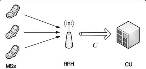
Fig. 1Uplink communication between a number of MSs and an RRH. The RRH is connected via a finite-capacity fronthaul link to a CU that performs baseband processing, including synchronization
compression in Section 3.3. Finally, the performance is evaluated through simulations to present benefits of the proposed compression scheme in Section 4.
1.1 Notation
Boldface lowercase letters denotes column vectors and boldface uppercase letters denotes matrices. The super-scripts(·)†denotes conjugate transpose of its argument. (·)−1 denotes inverse operation of its argument. The determinant of matrix A is denoted as|A|. The expec-tation operation with respect to x is denoted as Ex[·];
the correlation matrix of random vector xis defined as Kx=E[xx†].
2 System model
In this paper, we consider training-based synchronization for the uplink of a C-RAN cellular system. We specifically focus on the operation of a single cell, as illustrated in Fig. 1, and assume that, as in current cellular implemen-tations, the MSs transmit over orthogonal time/frequency resources, so that we can focus on a single active MS in a given resource block. The MS transmits a frame consist-ing of a trainconsist-ing and a data field. We further assume that the active MS and the RRH have a single antenna. The RRH is connected to a CU in the cloud via a fronthaul link that can deliverCbits per uplink sample to the CU. It is also assumed that the RRH is synchronized at the frame level so as to be able to distinguish between the training and data fields that compose each transmitted frame.
2.1 Training phase
Assuming a flat-fading channel, the signal received at the RRH during the training, or pilot, field, is given as
yp(t)=Aejθ Np−1
l=−L+1
xp[l]g(t−lT−τ)+zp(t),t∈[0,NpT)
(1)
where A is a positive amplitude that accounts for the attenuation due to fading; θ is the phase offset, which models the effect of the channel and of the phase mis-match between the oscillators at the MS and at the RRH; τ accounts for the residual timing offset between MS and RRH;Tis the symbol period;xp[l] is thelth pilot symbol
transmitted by the MS;Np is the number of pilot
sym-bols;g(t)is the pulse shape, which includes the effect of the transmit and receive filter and is assumed to be sup-ported in the interval [ 0,(L−1)T] for some integerL>1; and zp(t) is the complex additive white Gaussian noise
with two-sided power spectral density N0. We assume that the RRH is able to estimate the channel amplitude
offsetτ and phase offsetθneed to be estimated from the received signal (1).
The training sequence is generated randomly such that the symbols xp[l] for l = 0, ...,Np−1 are independent
and distributed asCN(0,Exp). The training sequence is known to the CU and the random generation is assumed here for the sake of simplifying the analysis in the spirit of Shannon’s random coding (see, e.g., [16]). We further assume that the pilot symbols are preceded by a cyclic prefix of duration equal to(L− 1)T. This implies that
xp[−l]=xp[−l+Np] for 1≤l≤L−1. Alternatively, as
it will be discussed, the analysis below holds as long as the number of training symbolsNpis sufficiently larger than
the support of the waveformg(t)L.
In order to potentially enhance the performance of phase and time synchronization, we allow the receiver to oversample the received signal at the BS with a sampling period Ts = T/F, where F is the oversampling factor.
For simplicity of analysis, we consider a raised cosine pulse g(t) with zero excess bandwidth (i.e., a sinc func-tion) so that the two-sided bandwidth isB = 1/T. As a result, settingF = 1, i.e., no oversampling, is an accept-able choice that leads to no spectral aliasing. However, as it will be seen in Section 4, the selectionF > 1 may yield an improved performance. Note that this is true even under the given assumption of zero excessive bandwidth. The reason is that collecting a larger number of samples enables the mitigation of the effect of the additive noise.
The resulting discrete-time signalyp(mT+nTs)can be
expressed as the interleaving of theFpolyphase sequences
yn
p[m]= yp(mT+nTs), withn = 0, 1, ...,F−1, see, e.g.,
[17]. Each sequenceynp[m] can be in turn written as
ynp[m]=Axp[m]gnτ,θ[m]+znp[m] , m=0, ...,Np−1,
(2)
where we have definedznp[m]zp(mT+nTs),gτn,θ[m]
ejθg(mT+nT
s−τ), anddenotes the circular
convolu-tion. Assuming that the noisezp(t)is white over the
band-width [−1/2Ts, 1/2Ts], the discrete-time noise sequence
znp[m] is an i.i.d. process with zero mean and powerN0/Ts.
Remark 1The presampling filter has a cut-off frequency of 1/2T since it is matched to the signal waveform. As a result, the noise prior to sampling is bandlimited with two-sided bandwidth B = 1/T. As such, it is correlated with auto-correlation function proportional to sinc(t/T). Therefore, with oversampling, the discrete-time noise sam-ples, which are taken at times multiple of T/F, are more properly modelled as correlated if F > 1. Here, following many related references (see, e.g.,[18, 19]), we instead make the simplifying assumption that the noise is white. This choice can be seen to lead to lower bounds on the actual system performance.
2.2 Data phase
The signal received during the data field of a frame can be written, in an analogous fashion as (1), as
yd(t)=Aejθ Nd−1
l=−L+1
xd[l]g(t−lT−τ)+zd(t),t∈[0,NdT),
(3)
wherexd[l] is thelth data symbol transmitted by the MS,
which is generated randomly in a constellation setxwith
zero mean and powerExd, andNd is the number of data symbols. The other parameters are defined as in (1).
After sampling at baud rate for the data field, the discrete-time signal is given as
yd[m]=Aejθ
Nd−1
l=−L+1
xd[l]g((m−l)T−τ)+zd[m] ,
m=0, ...,Nd−1, (4)
where the discrete-time noise sequencezd[m] is an i.i.d.
process with zero mean and powerN0/T. Note that over-sampling could be adopted also for the data field by following the same model used for the training field, but we do not further pursue this here in order to focus on training for synchronization.
2.3 Fronthaul compression
Following the C-RAN principle, compression is per-formed at the RRH in order to convey the baseband signal over the limited-capacity fronthaul link to the CU. For the training field, we assume the use of block quantiz-ers that compress each nth polyphase sequence yn[m], with n = 0, ...,F − 1, separately for transmission over the fronthaul link. Note that, while joint compression of these sequences generally leads to an improved compres-sion efficiency, here we adopt separate comprescompres-sion both for its lower computation complexity and for its analyti-cal tractability. In particular, each polyphase sequence is stationary and can be hence compressed by using stan-dard compression strategies, including universal methods [15, Ch. 10]. Furthermore, the resulting compression rate can be computed using rates distortion theory as dis-cussed next.
Using the standard additive quantization noise model, the resulting compressed signal for each nth polyphase sequence can be written as
ˆ
ynp[m]=ynp[m]+qnp[m] , m=0, ...,Np−1, (5)
schemes can be designed such that the joint (empirical) distribution of the input and output of the quantizer sat-isfies (5), as long as the rate is sufficiently large (see, e.g., [16]). Furthermore, the relationship (5) can be in prac-tice approximated by a high-dimensional dithered vector quantizers [20]. The practical relevance of the additive-noise quantization model for system design is further validated in Section 4 by means of numerical results.
The covariance matrix Kqnp of the vector q
n
p =
qpn[ 0] , ...,qnp[Np−1]
is taken to be circulant in order to facilitate its optimization in the frequency domain. This is done with the aim of reducing the number of degrees of freedom in the problem, hence enabling efficient and scal-able optimization, as discussed in the next section. Taking the discrete Fourier transform (DFT) of (5) leads to the frequency-domain signals tively. Due to the lack of spectral aliasing afforded by the chosen waveform and sampling frequency, we can write
Gnτ,θ[k]=Gn[k]e−j(2π
k NpTsτ−θ).1
From the mentioned covering lemma [16] (see also [20]), the fronthaul rate required to convey the com-pressed signals yˆp = being similarly defined. However, the mutual information
I(yp;yˆp)depends on the joint distribution ofypandyˆpand hence on the timing offsetτ and phase offsetθ, which are not known at the RRH. Therefore, the necessary rate of a worst-case estimate isRp = supτ,θI(yp;yˆp). It can be
easily calculated from the mutual information, which is given by
. Since the covariance matrix of the quanti-zation noiseKqn
pis assumed to be circulant, by leveraging Szego theorem [21], we can write (7) as¨ power spectral density (PSD) of the quantization noise
qnp[m]. We observe that (8) does not depend on θ and τ. Therefore, the required fronthaul rate Rp is given by
the right-hand side of (8). We will therefore impose the fronthaul capacity constraint as
I(yp;yˆp)≤NpC, (9)
whereI(yp;yˆp)is given in (8).
The compressed data signal during the data field, similar to (5), can be written as
ˆ
yd[m]=yd[m]+qd[m] , m=0, ...,Nd−1, (10)
where qd[m] indicates the quantization noise, which is
assumed to be white Gaussian random variable with zero mean and varianceσq2d. We observe that an optimized cor-relation for the quantization noise on the data phase could also be designed, similar to [10], but we leave this aspect to future work in order to concentrate on training for synchronization. Furthermore, following the discussion above, the fronthaul rate required to convey the com-pressed data signalyˆd =[yˆd[ 0] , ...,yˆd[Nd−1] ], from the RRH to the CU is given by Rd = supτ,θI(yd;yˆd), with
vectorydbeing similarly defined, with
I(yd;yˆd)=log2|Kyd+Kqd|
where (11b) follows from Szego theorem as in (8) and the¨ fronthaul capacity constraint of the data phase is given as
I(yd;yˆd)≤NdC. (12)
3 Analysis and optimization
In this section, we analyze the performance of the C-RAN system introduced above by accounting for the impact of imperfect synchronization, with the aim of enabling the optimization of fronthaul quantization. We will first dis-cuss the performance of time and phase synchronization at the CU in Section 3.1. Then, we study the impact of syn-chronization errors on the SNR in Section 3.2. Finally, we investigate the optimization of fronthaul compression in Section 3.3.
3.1 CRBs for the time and phase offset estimation
The CU estimates the time and phase offsets based on the compressed pilot signalsyˆp, producing the estimates
ˆ
τ(yˆp,xp)andθ(ˆ yˆp,xp). The mean squared errors (MSEs)
of these estimates can be bounded by the corresponding CRBs, i.e., by the inequalities Eyˆp,xp[(τ(ˆ yˆp,xp)− τ)
CRBτ and Eyˆp,xp[(θ(ˆ yˆp,xp) − θ)2]≥ CRBθ. Note that
the mentioned estimates depend on both the training sequencexpand the compressed received signalyˆp, and
that the squared error is averaged over the joint distri-bution of xp and yˆp. To evaluate the CRBs, we assume
that the relationship (5)-(6) is satisfied for the given vec-tor quantizer. This is done for the sake of tractability and is motivated by the covering lemma and by the results in [20] as discussed in the previous section. The CRBs are given, respectively, as
The derivation of (13)–(14) is given in the Appendix. Note that the bounds (13) and (14) do not depend on the phaseθand delayτ.
3.2 Impact of the synchronization error on the SNR
Having estimated the time and phase offsetsτˆandθˆ, the CU compensates for these offsets in the received signal, obtaining the discrete-time signal
yd[m]=Aejθ synchronization errors for timing and phase, respectively. We note that compensation of the time offset requires interpolation, which is possible given the lack of spec-tral aliasing. Moreover, under the mentioned assumption on the zero excess bandwidth waveformg(t), the statis-tics of the (white Gaussian) noise terms are unchanged by interpolation.
To account for the impact of the synchronization errors τ andθ, we follow the approach in [22], whereby the sinc waveformg(t)is approximated by retaining only two sidelobes on either side. Under this approximation, we can express (15) as
yd[m]=Axd[m]g(τ)+zs[m]+zisi[m]+zd[m] ,
(16)
where the terms in (16) are detailed below. First, the term zs[m]= Axd[m]g(τ)(ejθ − 1) indicates
addi-tional noise caused by the estimation error of phase offset θ. The termzisi[m] instead accounts for inter-symbol
interference caused by the time synchronization error and is given as
andzisi[m], we make the simplifying assumption that the
estimation errors τ and θ are uniform distributed on We observe that this approximation is expected to be increasingly accurate in the regime of small synchroniza-tion errors. Moreover, we approximateτmaxandθmax by means of the CRBτ (13) and CRBθ (14), respectively, by imposing the equalitiesE[τ2]=CRBτandE[θ2]= CRBθ, which yieldsτmax = √12CRBτ and θmax =
√
12CRBθ. Finally, we adopt the piecewise linear approx-imation of the raised cosine pulseg(t)proposed in [22], whereby pulseg(t)can be written as
To evaluate the effect of the synchronization error on the performance, we now calculate an effective signal to noise ratio (SNR) that accounts for the presence of the estimation error for time and phase offsets. By using the discussion above, the following approximations are derived in the Appendix. The power of the desired signal
sd[m]=Axd[m]g(τ)in (16) is approximated as
Table 1Coefficients in the piecewise linear approximation of the raised cosine pulse
l m−3 m−2 m−1 m+1 m+2 m+3
a+l 0 c4 −c2 c1 −c3 c5
The power ofzs[m] in (16) is similarly approximated as
Using (20), (21), and (22), we obtain the approximate effective SNR expression we made the further approximationfτ ≈ 1. We observe that the expression (23b) captures the effect of time and phase errors by means of additional noise terms in the denominator of the effective SNR. We remark that the approximations made in deriving (23b) will be validated in the numerical results by evaluating the performance of proposed optimization schemes for fronthaul compres-sion that are based on (23b) and discussed next.
3.3 Optimization of fronthaul compression
In the proposed design, we wish to maximize the effec-tive SNR (23b) under the constraints (9) and (12) on the fronthaul capacity, over the statistics of the quantization noises, namely over the PSDsSQnp[k] of the training field and over the variance of the quantization noiseσ2
qdfor the data field. Accordingly, we have following optimization problem:
where constraints (24b) and (24c) correspond to (9) and (12), respectively.
Towards solving problem (24), we first observe that the varianceσq2
dcan be obtained, without loss of optimality, by imposing the equality in constraint (24c). This is because SNReff is monotonically decreasing with respect toσq2d while the left-hand side of (24c) is monotonically decreas-ing inσq2d. We then have the following equivalent problem
minimize
where the objective function (25a) can be rewritten, using (13) and (14), as
To tackle the optimization problem (25), we first define the auxiliary variables un,k (SQn[k])−1,
yielding the equivalent objective function
A2Exd
The objective function (27) is convex with respect to the variablesvn,k since denominator of each term is an affine function ofvn,k, and the function 1/g(x)is convex ifg(x)
is concave and positive. However, the constraint (25b) is still not convex in the variablesvn,kforn=0, ...,F−1,k=
0, ...,Np−1. Nevertheless, it can be expressed as the sum
of a concave and of a convex function, i.e.,
Algorithm 1DC algorithm for problem (25)
1: Initialization:i = 0 andvn(0,k) = 1 forn = 0, ...,F−
1,k=0, ...,Np−1
2: Obtain{v(ni+,k1)}n,kas a solution of the following convex
problem:
minimize
vn,k ( 27)
s.t.
F−1
n=0
Np−1
k=0
e(ni,)kvn,k+fn(i,k)−log2((N0/Ts)vn,k
≤NpC,
0≤vn,k ≤1, ∀n,k (28)
3: Seti=i+1
4: If a convergence criterion is satisfied, stop; otherwise, go to step 2. Return the obtained solutionv(ni,)kforn=
0, ...,F−1,k=0, 1, ...,Np−1.
Therefore, the Difference of Convex (DC) approach [15] can be leveraged to obtain an iterative optimization algo-rithm. This is done by linearizing the concave part of (29) at the current iteratev(ni,)k, whereiis the index of the cur-rent iteration, obtaining the locally tight convex upper bound
log2(−bn,kvn,k+bn,k+N0/Ts)≤e(ni,)kvn,k+fn(,ik), (30)
wheree(ni,)k = −bn,k/(ln(2)(NT0s +bn,k −bn,kvn(i,)k)),fn(,ik) =
log2(−bn,kv(ni,)k+bn,k+NT0s)−e
(i) n,kv
(i) n,k.
The DC algorithm performs successive optimization of the convex problem obtained by substituting the right-hand side of (30) for the concave part in (29) until conver-gence. Given the known properties of the DC algorithm [15], the proposed approach, summarized in Algorithm 1, provides a feasible solution at every iteration and con-verges to a local minimum of problem (25). Moreover, since it only requires the solution of convex problems, the algorithm has a polynomial complexity per iteration.
4 Numerical results
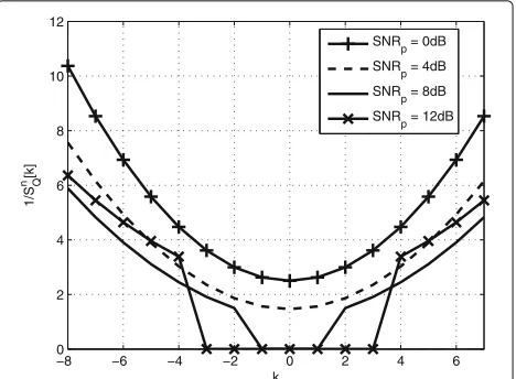
In this section, we present numerical results to give insight into optimal fronthaul compression for synchronization and to validate the analysis presented in the previous sections. Throughout, we setA = 0.7 and the SNR dur-ing traindur-ing phase and SNR durdur-ing data phase are defined as SNRp = Exp/(N0/Ts) and SNRd = Exd/(N0/T), respectively.
Figure 2 shows the inverse of the PSD of the quantiza-tion noise 1/SQn
p[k] obtained from Algorithm 1 for various values of SNRpwithC = 3 bits/sample,N = 100,Np =
16, andF = 2. Note that the frequency axis ranges from
−Np/2 toNp/2−1 rather than in the interval [0,Np−1]
−8 −6 −4 −2 0 2 4 6
0 2 4 6 8 10 12
k
1/S
n[k]Q
SNR
p = 0dB
SNR
p = 4dB
SNR
p = 8dB
SNR
p = 12dB
Fig. 2Inverse of the PSD of the quantization noise obtained from Algorithm 1 versus the frequency indexk:C=3 bits/sample, F=2,A=0.7,N=100 andNp=16
for convenience of illustration. Moreover, we emphasize that 1/SQnp[k] is a measure of the accuracy of quantiza-tion at frequency k with k = −Np/2, ...,Np/2− 1, so
that a larger 1/SQn
p[k] implies a more refined quantization. We first observe that the optimized solution prescribes a more accurate quantization at higher frequencies, since these convey more information on the time delay, as per the CRB (13), while all frequencies contribute in equal manner to the estimate of the phase offset as per (14). Moreover, as SNRpincreases, it is seen that lower
frequen-cies tend to be neglected by the quantizer in the sense that, for such frequencies, we have 1/SQn
p[k]=0, and hence the signals on these frequencies are not compressed and not transmitted to the CU.
In order to validate the advantage of the proposed design, we now consider the synchronization performance under a conventional least-square joint phase and timing estimator operating on the compressed signalYˆn[k] ,n=
0,. . .,F−1,k=0,. . .,Np−1. The estimator is given as (θˆ,τ)ˆ =arg min
˜ θ,τ˜ (
˜
θ,τ)˜ , (31)
with (θ˜,τ)˜ = n,k|rnk − rkn(θ˜,τ)˜ |2 where rnk =
arg(Yˆn[k]X∗[k])/2π andrkn(θ˜,τ)˜ = ˜θ −k/Np(n+ ˜τ).
By applying the estimator (31), we evaluate the perfor-mance of optimized compression scheme in terms of MSEs of time and phase offsets as compared to white-PSD compression that is constant across all frequencies. The white-PSD compression scheme is considered as ref-erence since it does not attempt to optimize quantization with the aim of enhancing synchronization.
a
b
c
d
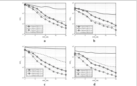
Fig. 3MSE for joint phase and timing estimation (31) versus theSNRp:A=0.7,N=100 andNp=16aF=1, MSE of phase offset.bF=1, MSE of phase offset.cF=2, MSE of timing offset.dF=2, MSE of phase offset
C = 1 bits/sample and C = 3 bits/sample with F =
1,A = 0.7,N = 100, and Np = 16. In addition, we
plot the MSE of the timing and phase offset estimates in case ofF = 2 in Fig. 3c, 3d, respectively, under the same parameters. We observe that the proposed scheme signif-icantly outperforms the conventional white-PSD strategy and that the gain of the proposed scheme is more pro-nounced for larger SNR values. This is because as the SNR grows, the impact of the quantization noise becomes more relevant compared to the channel noise. Furthermore, a larger oversampling factorF seems to yield an improved performance only for the proposed optimization scheme and not with the conventional white-PSD scheme. This is because in the latter case, the performance benefits of a larger number of observation are offset by the increased fronthaul overhead, which leads to a more pronounced quantization noise.
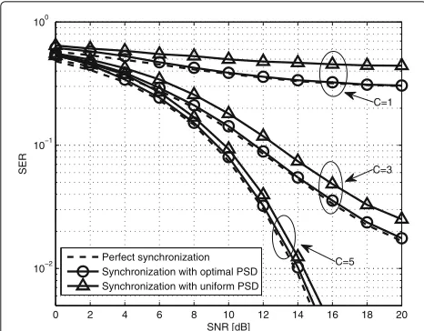
Adopting the same estimator for time and phase offset, the system performance in terms of uncoded SER dur-ing the data phase is shown in Figs. 4 and 5 for BPSK and QPSK modulation, respectively. We consider the SNR for both training and data fields, i.e., SNR = SNRp =
SNRd,F = 2,A = 0.7,N = 100 and Np = 16.
Simulation results with perfect synchronization are also presented for reference. We note that, consistently with
the results in Fig. 5, the proposed method is observed to outperform the conventional white-PSD scheme more significantly as the SNR increases and as the fronthaul capacity C decreases. For instance, it is seen in Fig. 5 that the proposed approach has a gain of about 0.5 dB
0 2 4 6 8 10 12 14 16 18 10−4
10−3 10−2 10−1 100
SNR [dB]
SER
Perfect synchronization Synchronization with optimal PSD Synchronization with uniform PSD
C=3 C=1
C=5
0 2 4 6 8 10 12 14 16 18 20 10−2
10−1 100
SNR [dB]
SER
Perfect synchronization Synchronization with optimal PSD Synchronization with uniform PSD
C=5 C=1
C=3
Fig. 5SER with uncoded QPSK transmission versus SNR with joint phase and timing estimation (31):F=2,A=0.7,N=100 andNp=16
for C = 5 bits/sample and of about 2 dB for C = 3 bits/sample.
Finally, we elaborate on the performance of actual quan-tization by adopting a standard scalar uniform quantizer, instead of the additive quantization model considered so far. In particular, we choose the step size [k] of the quantizer used for frequency k based on the opti-mal PSDSq[k] obtained from Algorithm 1 by using the
relationshipSq[k]= |[k]| 2
12 . This relationship is justified by fact that, at high resolution, the quantization noise is approximately uniformly distributed. As reference, we also consider the performance of a uniform quantizer in which step size is same for all frequenciesk, i.e.,[k]= , with the same dynamic range as for the optimized quantizer. Figure 6 presents the MSE of the timing and
0 2 4 6 8 10 12 14 16 18 20 10−4
10−3 10−2 10−1
SNR p [dB]
MSE
Scalar uniform quantizer with optimal step size Scalar uniform quantizer with constant step size
MSE of θ
MSE of τ
Fig. 6MSE of joint phase and timing estimation versusSNRpin the presence of scalar fronthaul quantization and joint phase and timing estimation (31):F=2,C=3,A=0.7,N=100 andNp=16
phase offset estimates versus SNRp with F = 2,C =
3,A = 0.7,N = 100 andNp = 16. We observe that
the proposed scheme outperforms the conventional uni-form quantizer, with a gain of about 2 dB in the high SNR regime.
5 Conclusions
This paper tackles the problem of optimal fronthaul compression with the aim of enhancing the effective SNR in the presence of time and phase synchroniza-tion errors at the CU. The proposed algorithm optimizes the PSD of quantization noise at the RRHs by using the Charnes-Cooper transformation and the DC approach, and is shown to outperform the conventional solution that assumes an equal quantizer at all frequencies. Numerical results validate the analysis by evaluating the perfor-mance of the proposed design under practical synchro-nization algorithms and with scalar quantization. An interesting direction for future research is the consider-ation of frequency-selective channels and of frequency synchronization.
Endnote
1The more general case with spectral aliasing could be
handled by using the analysis in [17] and is left as an open problem.
6 Appendix
6.1 Proof of the CRBs for time and phase offset estimates
In this appendix, we provide a brief derivation for the bounds (13) and (14), which follow from standard argu-ments (see, e.g., [23]). For the bound (13), we first have the chain of inequalities
Eyˆp,xp[τ(yˆp) 2]=E
xp[Eyˆp|xp[τ(yˆp)
2] ] (32)
≥Exp
⎡ ⎢ ⎢
⎣ 1
Eyˆp|xp
∂lnp(yˆ
p|xp,τ)
∂τ
2
⎤ ⎥ ⎥ ⎦
(33)
≥ 1
Exp
Eyˆp|xp
∂lnp(yˆ
p|xp,τ)
∂τ
2,
(34)
of correlated Gaussian observations can be calculated using [24, Ch. 3.9] , which can be directly evaluated as
Eyˆp|xp
The summation in (35) follows from the fact that the vectorsyˆnp inyˆp =[yˆ0p,· · ·,yˆF−p 1] are independent for all
n given the pilot signalxp. Furthermore, in (35), Kz˜n is
the covariance matrix of the effective noisez˜n = znp+qnp and we have definedsn =[sn[ 0] , ...,sn[Np− 1] ]T with
sn[m]= Axp[m]gτn,θ[m]. Finally, equality (36) follows
from Szego theorem. By inserting (36) into (34), and not-¨ ing thatE[|X[k]|2]=Exp, the proof of (13) is concluded. The proof of (14) can be obtained using similar steps and is omitted.
6.2 Derivation of (20), (21), and (22)
We compute the powers of the desired signalsd[m] in (20)
and of the interference termszs[m] in (21) and ofzisi[m]
in (22). The power of the desired signal is approximated, using (19), as
where in (37c) we used the assumption τ ∼
U[−τmax
2 ,τ2max], which implies E[|τ|]= τ4max and
E[|τ|2]= τmax2
12 ; (37d) follows by removing higher-order terms inτmaxunder the assumption thatτmaxis small enough; and (37e) is a consequence of the approximation
E[τ2]= τmax2
12 ≈CRBτ.
The power of zs[m] is similarly approximated, using
(19), as
where the approximation in (38b) follows as
Eθ[|e−jθ−1|2]=2−2Eθ[ cos(θ)] (39a)
where (39c) follows from the Taylor series of the sinc func-tion up to the second order, and (39e) is a consequence of the approximationE[θ2]= θmax2
12 ≈CRBθ.
Finally, using (18a), the power ofzisi[m] is approximated
as
The work of O. Simeone was partially supported by U.S. NSF under grant CCF-1525629. This work was supported by ’The Cross-Ministry Giga KOREA Project’ grant from the Ministry of Science, ICT, and Future Planning, Korea.
Competing interests
The authors declare that they have no competing interests.
Author details
1School of Electrical Engineering, Korea Advanced Institute of Science and
Technology (KAIST), 291 Daehak-ro, Yuseong-gu, Daejeon 34141, Republic of Korea.2Center for Wireless Information Processing (CWIP), Electrical and Computer Engineering Department, New Jersey Institute of Technology (NJIT), Newark, NJ, USA.
Received: 6 October 2015 Accepted: 2 January 2017
References
2. A Checko, HL Christiansen, Y Yan, L Scolari, G Kardaras, MS Berger, L Dittmann, Cloud RAN for mobile networks: A technology overview. IEEE Comm. Surv. Tutorials.17(1), 405–426 (2012)
3. AB Ericsson. Huawei Technologies, NEC Corporation, Alcatel Lucent and Nokia Siemens Networks, Common public radio interface (CPRI); interface specification, CPRI specification. vol. 5, (2011)
4. D Samardzija, J Pastalan, M MacDonald, S Walker, R Valenzuela, Compressed transport of baseband signals in radio access networks. IEEE Trans. Wirel. Comm.11(9), 3216–3225 (2012)
5. B Guo, W Cao, A Tao, D Samardzija, inProc. Int. ICST Conf. CHINACOM. CPRI compression transport for LTE and LTE-A signal in C-RAN, (2012), pp. 843–849
6. A Vosoughi, M Wu, JR Cavallaro, inProc. IEEE Global Communications Conference. Baseband signal compression in wireless base stations, (2012), pp. 4505–4511
7. A Sanderovich, O Somech, HV Poor, S Shamai, Uplink macro diversity of limited backhaul cellular network. IEEE Trans.Inf. Theory.55(8), 3457–3478 (2009)
8. L Zhou, W Yu, Optimized backhaul compression for uplink Cloud Radio Access Network. IEEE J. Sel. Areas Comm.32(6), 1295–1307 (2014) 9. A del Coso, S Simoens, Distributed compression for MIMO coordinated
networks with a backhaul constraint. IEEE Trans. Wirel. Comm.8(9), 4698–4709 (2009)
10. S-H Park, O Simeone, O Sahin, S Shamai, Robust and efficient distributed compression for cloud radio access networks. IEEE Trans. Veh. Techn.62(2), 692–703 (2013)
11. J Hoydis, M Kobayashi, M Debbah, Optimal channel training in uplink network MIMO systems. IEEE Trans. Sig. Proc.59(6), 2824–2833 (2011) 12. J Kang, O Simeone, J Kang, S Shamai, Joint signal and channel state
information compression for the backhaul of uplink network MIMO systems. IEEE Trans. Wirel. Comm.13(3), 1555–1567 (2014)
13. S-H Park, O Simeone, O Sahin, S Shamai, Fronthaul compression for cloud radio access networks: signal processing advances inspired by network information theory. IEEE Signal Proc. Mag.31(6), 69–79 (2014)
14. A Charnes, WW Cooper, Programming with linear fractional functionals. Nav. Res. Logist. Q.9(3–4), 181–186 (1962)
15. R Horst, NV Thoai, DC Programming: Overview. J. Optim. Theory Appl. 103(1), 1–43 (1999)
16. A El Gamal, Y Kim,Network information theory. (Cambridge University Press, 2012)
17. Y Chen, YC Eldar, AJ Goldsmith, Shannon meets Nyquist: Capacity of sampled Gaussian channels. IEEE Trans. Inf. Theory.69(8), 4889–4914 (2013) 18. L Tong, G Xu, B Hassibi, T Kailath, Blind channel identification based on
second-order statistics: A frequency-domain approach. IEEE Trans. Inf. Theory.41(1), 329–334 (1995)
19. S Gault, W Hachem, P Ciblat, inProc. IEEE ICASSP. Cramer-Rao bounds for data-aided sampling clock offset and channel estimation, vol. 4, (2004), pp. iv-1029-32
20. R Zamir, M Feder, On lattice quantization noise. IEEE Trans. Inf. Theory. 42(4), 1152–1159 (1996)
21. RM Gray,Toeplitz and Circulant Matrices: A review. (Now Publishers Inc, 2006)
22. S Jagannathan, H Aghajan, A Goldsmith, inProc. IEEE GLOBECOM 2004. The effect of time synchronization errors on the performance of cooperative MISO systems, (2004), pp. 102–107
23. F Gini, R Reggiannini, U Mengali, The modified Cramer-Rao bound in vector parameter estimation. IEEE Trans. Comm.46(1), 52–60 (1998) 24. SM Kay,Fundamentals of Statistical Signal Processing: Estimation Theory.
(Prentice-Hall, Englewood Cliffs, NJ, 1993)
Submit your manuscript to a
journal and benefi t from:
7Convenient online submission 7Rigorous peer review
7Immediate publication on acceptance 7Open access: articles freely available online 7High visibility within the fi eld
7Retaining the copyright to your article