Volume 2008, Article ID 868425,29pages doi:10.1155/2008/868425
Research Article
Neural Network Adaptive Control for Discrete-Time
Nonlinear Nonnegative Dynamical Systems
Wassim M. Haddad,1 VijaySekhar Chellaboina,2 Qing Hui,1
and Tomohisa Hayakawa3
1School of Aerospace Engineering, Georgia Institute of Technology, Atlanta, GA 30332-0150, USA 2Department of Mechanical and Aerospace Engineering, University of Tennessee, Knoxville,
TN 37996-2210, USA
3Department of Mechanical and Environmental Informatics (MEI), Tokyo Institute of Technology, O’okayama, Tokyo 152-8552, Japan
Correspondence should be addressed to W. M. Haddad,[email protected] Received 27 January 2008; Accepted 8 April 2008
Recommended by John Graef
Nonnegative and compartmental dynamical system models are derived from mass and energy balance considerations that involve dynamic states whose values are nonnegative. These models are widespread in engineering and life sciences, and they typically involve the exchange of nonnegative quantities between subsystems or compartments, wherein each compartment is assumed to be kinetically homogeneous. In this paper, we develop a neuroadaptive control framework for adaptive set-point regulation of discrete-time nonlinear uncertain nonnegative and compartmental systems. The proposed framework is Lyapunov-based and guarantees ultimate boundedness of the error signals corresponding to the physical system states and the neural network weighting gains. In addition, the neuroadaptive controller guarantees that the physical system states remain in the nonnegative orthant of the state space for nonnegative initial conditions.
Copyrightq2008 Wassim M. Haddad et al. This is an open access article distributed under the Creative Commons Attribution License, which permits unrestricted use, distribution, and reproduction in any medium, provided the original work is properly cited.
1. Introduction
nonnegative dynamical systems are compartmental systems 8–18. Compartmental systems involve dynamical models that are characterized by conservation laws e.g., mass and energycapturing the exchange of material between coupled macroscopic subsystems known as compartments. The range of applications of nonnegative systems and compartmental systems includes pharmacological systems, queuing systems, stochastic systems whose state variables represent probabilities, ecological systems, economic systems, demographic systems, telecommunications systems, and transportation systems, to cite but a few examples. Due to the severe complexities, nonlinearities, and uncertainties inherent in these systems, neural networks provide an ideal framework for online adaptive control because of their parallel processing flexibility and adaptability.
In this paper, we extend the results of2to develop a neuroadaptive control framework for discrete-time nonlinear uncertain nonnegative and compartmental systems. The proposed framework is Lyapunov-based and guarantees ultimate boundedness of the error signals corresponding to the physical system states as well as the neural network weighting gains. The neuroadaptive controllers are constructed without requiring knowledge of the system dynamics while guaranteeing that the physical system states remain in the nonnegative orthant of the state space. The proposed neuro control architecture is modular in the sense that if a nominal linear design model is available, the neuroadaptive controller can be augmented to the nominal design to account for system nonlinearities and system uncertainty. Furthermore, since in certain applications of nonnegative and compartmental systemse.g., pharmacological systems for active drug administration control sourceinputs as well as the system states need to be nonnegative, we also develop neuroadaptive controllers that guarantee the control signal as well as the physical system states remain nonnegative for nonnegative initial conditions.
The contents of the paper are as follows. In Section 2, we provide mathematical preliminaries on nonnegative dynamical systems that are necessary for developing the main results of this paper. In Section 3, we develop new Lyapunov-like theorems for partial boundedness and partial ultimate boundedness for nonlinear dynamical systems necessary for obtaining less conservative ultimate bounds for neuroadaptive controllers as compared to ultimate bounds derived using classical boundedness and ultimate boundedness notions. In Section 4, we present our main neuroadaptive control framework for adaptive set-point regulation of nonlinear uncertain nonnegative and compartmental systems. In Section 5, we extend the results of Section 4 to the case where control inputs are constrained to be nonnegative. Finally, inSection 6we draw some conclusions.
2. Mathematical preliminaries
In this section we introduce notation, several definitions, and some key results concerning linear and nonlinear discrete-time nonnegative dynamical systems19that are necessary for developing the main results of this paper. Specifically, for x ∈ Rn we write x ≥≥ 0 resp.,
x >>0to indicate that every component ofxis nonnegativeresp., positive. In this case, we say thatxisnonnegativeorpositive, respectively. Likewise,A ∈ Rn×m isnonnegativeorpositive if every entry of A is nonnegative or positive, respectively, which is written as A ≥≥ 0 or
A >>0, respectively. In this paper it is important to distinguish between a square nonnegative
resp., positivematrix and a nonnegative-definiteresp., positive-definitematrix. LetRnand
Rn
x ∈ Rn
are equivalent, respectively, to x ≥≥ 0 and x >> 0. Finally, we write ·T to denote transpose, tr· for the trace operator, λmin· resp., λmax· to denote the minimum resp.,
maximumeigenvalue of a Hermitian matrix, ·for a vector norm, andZ for the set of all nonnegative integers. The following definition introduces the notion of a nonnegativeresp., positivefunction.
Definition 2.1. A real functionu:Z→Rmis anonnegativeresp.,positivefunctionifuk≥≥0
resp.,uk>>0,k ∈Z.
The following theorems give necessary and sufficient conditions for asymptotic stability of the discrete-time linear nonnegative dynamical system
xk1 Axk, x0 x0, k ∈Z, 2.1
where A ∈ Rn×n is nonnegative andx 0 ∈ R
n
, usinglinearandquadraticLyapunov functions, respectively.
Theorem 2.2see19. Consider the linear dynamical systemG given by2.1whereA ∈ Rn×n is nonnegative. ThenGis asymptotically stable if and only if there exist vectorsp, r∈Rnsuch thatp >>0
andr >>0satisfy
p ATpr. 2.2
Theorem 2.3see6,19. Consider the linear dynamical systemGgiven by2.1whereA ∈Rn×n is nonnegative. Then G is asymptotically stable if and only if there exist a positive diagonal matrix
P ∈Rn×nand ann×npositive-definite matrixRsuch that
P ATP AR. 2.3
Next, consider the controlled discrete-time linear dynamical system
xk1 Axk Buk, x0 x0, k∈Z, 2.4
where
B
B
0n−m×m
, 2.5
A ∈ Rn×n is nonnegative and B ∈ Rm×m is nonnegative such that rank B m. The following theorem shows that discrete-time linear stabilizable nonnegative systems possess asymptotically stable zero dynamics with x x1, . . . , xm viewed as the output. For the statement of this result, let specAdenote the spectrum of A, let C1 {s ∈ C : |s| ≥ 1},
and letA∈Rn×nin2.4be partitioned as
A
A11 A12
A21 A22
, 2.6
where A11 ∈ Rm×m, A12 ∈ Rm×n−m, A21 ∈ Rn−m×m, and A22 ∈ Rn−m×n−m are nonnegative
Theorem 2.4. Consider the discrete-time linear dynamical systemGgiven by2.4, whereA ∈Rn×n is nonnegative and partitioned as in2.6, andB∈Rn×mis nonnegative and is partitioned as in2.5 with rankB m. Then there exists a gain matrixK ∈ Rm×n such thatABKis nonnegative and asymptotically stable if and only ifA22is asymptotically stable.
Proof. First, letKbe partitioned asK K1, K2, whereK1 ∈ Rm×m andK2 ∈ Rm×n−m, and
note that
ABKT
⎡ ⎣
A11BK 1
T
AT21
A12BK 2
T
AT22 ⎤
⎦. 2.7
Assume thatABKis nonnegative and asymptotically stable, and suppose that,ad absurdum,
A22is not asymptotically stable. Then, it follows fromTheorem 2.2that there does not exist a
positive vectorp2 ∈Rn−m such thatAT22−Ip2 << 0. Next, sinceA12BK 2 is nonnegative it
follows that A12BK 2Tp1 ≥≥ 0 for any positive vectorp1 ∈Rm. Thus, there does not exist a positive vectorp pT1, pT2T such that ABKT −Ip << 0, and hence, it follows from Theorem 2.2thatABK is not asymptotically stable leading to a contradiction. Hence,A22
is asymptotically stable. Conversely, suppose that A22 is asymptotically stable. Then taking
K1 B−1As −A11andK2 −B−1A12, whereAs is nonnegative and asymptotically stable,
it follows that specABK∩C1 specAs∪specA22∩C1 Ø, and hence, ABK is
nonnegative and asymptotically stable.
Next, consider the discrete-time nonlinear dynamical system
xk1 fxk, x0 x0, k∈Z, 2.8
wherexk ∈ D,Dis an open subset ofRnwith 0 ∈ D, andf : D → Rn is continuous onD. Recall that the pointxe∈ Dis anequilibrium pointof2.8ifxe fxe. Furthermore, a subset
Dc ⊆ D is an invariant set with respect to2.8if Dc contains the orbits of all its points. The
following definition introduces the notion of nonnegative vector fields19.
Definition 2.5. Letf f1, . . . , fnT :D →Rn, whereDis an open subset ofRnthat containsR n . Thenfisnonnegative with respect toxx1, . . . , xmT,m≤n, iffix≥0 for alli 1, . . . , m, and
x∈Rn.fisnonnegativeiffix≥0 for alli 1, . . . , n, andx∈R n .
Note that if fx Ax, where A ∈ Rn×n, then f is nonnegative if and only if A is nonnegative19.
Proposition 2.6see19. SupposeRn⊂ D. ThenRnis an invariant set with respect to2.8if and only iff:D →Rnis nonnegative.
In this paper, we consider controlled discrete-time nonlinear dynamical systems of the form
xk1 fxkGxkuk, x0 x0, k ∈Z, 2.9
wherexk∈Rn,k ∈Z
,uk∈Rm,k ∈Z,f :Rn → Rnis continuous and satisfiesf0 0, andG:Rn→Rn×mis continuous.
Definition 2.7. The discrete-time nonlinear dynamical system given by2.9isnonnegativeif for everyx0∈Rnanduk≥≥0,k∈Z, the solutionxk,k∈Z, to2.9is nonnegative.
Proposition 2.8 see 19. The discrete-time nonlinear dynamical system given by 2.9 is nonnegative iffx≥≥0andGx≥≥0,x∈Rn.
It follows fromProposition 2.8that a nonnegative input signal Gxkuk, k ∈ Z, is sufficient to guarantee the nonnegativity of the state of2.9.
Next, we present a time-varying extension to Proposition 2.8 needed for the main theorems of this paper. Specifically, we consider the time-varying system
xk1 fk, xkGxkuk, xk0 x0, k ≥k0, 2.10
where f : Z×Rn → Rn is continuous in k andx onZ×Rn andfk,0 0, k ∈ Z, and
G : Rn → Rn×mis continuous. For the following result, the definition of nonnegativity holds with2.9replaced by2.10.
Proposition 2.9. Consider the time-varying discrete-time dynamical system 2.10 where fk,· :
Rn→Rnis continuous onRnfor allk∈Z
andf·, x:Z→Rnis continuous onZfor allx∈Rn. If for everyk ∈ Z,fk,· : Rn → Rn is nonnegative andG : Rn → Rn×m is nonnegative, then the solutionxk,k≥k0, to2.10is nonnegative.
Proof. The result is a direct consequence of Proposition 2.8 by equivalently representing the time-varying discrete-time system2.10as an autonomous discrete-time nonlinear system by appending another state to represent time. Specifically, definingyk−k0xkandyn1k−
k0k, it follows that the solutionxk,k≥k0, to2.10can be equivalently characterized by
the solutionyκ,κ≥0, whereκk−k0, to the discrete-time nonlinear autonomous system
yκ1 fyn1κ, yκ
Gyκuκ, y0 y0, κ≥0, 2.11
yn1κ1 yn1κ 1, yn10 k0, 2.12
whereuκuκk0. Now, sinceyiκ≥0,κ≥0, fori 1, . . . , n1, andGxκuκ≥≥0, the result is a direct consequence ofProposition 2.8.
3. Partial boundedness and partial ultimate boundedness
In this section, we present Lyapunov-like theorems forpartial boundednessandpartial ultimate boundednessof discrete-time nonlinear dynamical systems. These notions allow us to develop less conservative ultimate bounds for neuroadaptive controllers as compared to ultimate bounds derived using classical boundedness and ultimate boundedness notions. Specifically, consider the discrete-time nonlinear autonomous interconnected dynamical system
x1k1 f1
x1k, x2k
, x10 x10, k ∈Z, 3.1
x2k1 f2
x1k, x2k
, x20 x20, 3.2
wherex1 ∈ D,D ⊆ Rn1 is an open set such that 0 ∈ D,x2 ∈ Rn2,f1 : D ×Rn2 → Rn1 is such
that, for everyx2∈Rn2,f10, x2 0 andf1·, x2is continuous inx1, andf2 :D ×Rn2 →Rn2
is continuous. Note that under the above assumptions the solutionx1k, x2kto3.1and
Definition 3.1 see 20. i The discrete-time nonlinear dynamical system 3.1and 3.2 is
bounded with respect to x1 uniformly inx20 if there exists γ > 0 such that, for everyδ ∈ 0, γ,
there existsε εδ>0 such thatx10< δimpliesx1k< εfor allk∈Z. The discrete-time nonlinear dynamical system3.1and3.2isglobally bounded with respect tox1uniformly inx20
if, for everyδ∈0,∞, there existsε εδ>0 such thatx10< δimpliesx1k< εfor all
k∈Z.
iiThe discrete-time nonlinear dynamical system 3.1 and3.2 isultimately bounded with respect tox1uniformly inx20with ultimate boundεif there existsγ >0 such that, for every
δ ∈ 0, γ, there exists K Kδ, ε > 0 such that x10 < δ implies x1k < ε, k ≥ K.
The discrete-time nonlinear dynamical system3.1and3.2isglobally ultimately bounded with respect to x1 uniformly in x20 with ultimate bound ε if, for every δ ∈ 0,∞, there exists K
Kδ, ε>0 such thatx10< δimpliesx1k< ε,k ≥K.
Note that if a discrete-time nonlinear dynamical system is globally bounded with respect to x1 uniformly in x20, then there exists ε > 0, such that it is globally ultimately
bounded with respect tox1uniformly inx20with an ultimate boundε. Conversely, if a
discrete-time nonlinear dynamical system isgloballyultimately bounded with respect tox1uniformly
in x20 with an ultimate bound ε, then it isgloballybounded with respect to x1 uniformly
in x20. The following results present Lyapunov-like theorems for boundedness and ultimate
boundedness for discrete-time nonlinear systems. For these results define ΔVx1, x2
Vfx1, x2− Vx1, x2, where fx1, x2 f1Tx1, x2, f2Tx1, x2T and V : D × Rn2 → R
is a given continuous function. Furthermore, letBδx, x ∈ Rn,δ > 0, denote the open ball centered atxwith radiusδand letBδxdenote the closure ofBδx, and recall the definitions of class-K, class-K∞, and class-KLfunctions20.
Theorem 3.2. Consider the discrete-time nonlinear dynamical system 3.1and 3.2. Assume that there exist a continuous functionV :D ×Rn2 →Rand class-Kfunctionsα·andβ·such that
αx1≤Vx1, x2≤βx1, x1∈ D, x2∈Rn2, 3.3
ΔVx1, x2
≤0, x1∈ D, x1> μ, x2∈Rn2, 3.4
whereμ >0is such thatBα−1βμ0⊂ D. Furthermore, assume thatsupx
1,x2∈Bμ0×Rn2Vfx1, x2
exists. Then the discrete-time nonlinear dynamical system3.1and3.2is bounded with respect tox1 uniformly inx20. Furthermore, for everyδ ∈ 0, γ,x10 ∈ Bδ0implies that x1k ≤ ε, k ∈ Z, where
ε εδα−1maxη, βδ, 3.5
η ≥ max{βμ,supx1,x2∈Bμ0×Rn2Vfx1, x2} max{βμ,supx1,x2∈Bμ0×Rn2Vx1, x2 ΔVx1, x2}, andγ sup{r >0 :Bα−1βr0⊂ D}. If, in addition,D Rn1 andα·is a class-K∞
function, then the discrete-time nonlinear dynamical system3.1and3.2is globally bounded with respect tox1uniformly inx20and for everyx10∈Rn1,x1k ≤ε,k ∈Z, whereεis given by3.5 withδ x10.
Theorem 3.3. Consider the discrete-time nonlinear dynamical system 3.1and3.2. Assume there exist a continuous function V : D ×Rn2 → R and class-Kfunctions α·andβ·such that3.3
holds. Furthermore, assume that there exists a continuous functionW :D →Rsuch thatWx1>0,
x1> μ, and
ΔVx1, x2
≤ −Wx1
, x1∈ D,x1> μ, x2∈Rn2, 3.6 where μ > 0 is such that Bα−1βμ0 ⊂ D. Finally, assume supx
1,x2∈Bμ0×Rn2Vfx1, x2 exists.
Then the nonlinear dynamical system3.1, 3.2is ultimately bounded with respect to x1 uniformly in x20 with ultimate bound ε α−1η, where η > max{βμ,supx1,x2∈Bμ0×Rn2Vfx1, x2}
max{βμ,supx1,x2∈Bμ0×Rn2Vx1, x2 ΔVx1, x2}. Furthermore, lim supk→∞x1k ≤
α−1η. If, in addition,D Rnandα·is a class-K
∞function, then the nonlinear dynamical system
3.1and3.2is globally ultimately bounded with respect tox1uniformly inx20with ultimate bound
ε.
Proof. See20, page 787.
The following result on ultimate boundedness of interconnected systems is needed for the main theorems in this paper. For this result, recall the definition of input-to-state stability given in21.
Proposition 3.4. Consider the discrete-time nonlinear interconnected dynamical system 3.1 and
3.2. If 3.2is input-to-state stable withx1 viewed as the input and3.1and3.2are ultimately bounded with respect to x1 uniformly in x20, then the solution x1k, x2k, k ∈ Z, of the interconnected dynamical system3.1-3.2, is ultimately bounded.
Proof. Since system3.1-3.2is ultimately bounded with respect tox1uniformly inx20, there
exist positive constantsεandK Kδ, εsuch thatx1k< ε,k≥K. Furthermore, since3.2
is input-to-state stable withx1 viewed as the input, it follows thatx2Kis finite, and hence,
there exist a class-KLfunctionη·,·and a class-Kfunctionγ·such that
x2k≤ηx2K, k−K
γmax
K≤i≤k
x1i
< ηx2K, k−K
γε
≤ηx2K,0
γε, k≥K,
3.7
which proves that the solutionx1k, x2k,k ∈Zto3.1and3.2is ultimately bounded.
4. Neuroadaptive control for discrete-time nonlinear nonnegative uncertain systems
In this section, we consider the problem of characterizing neuroadaptive feedback control laws for discrete-time nonlinear nonnegative and compartmental uncertain dynamical systems to achieve set-point regulation in the nonnegative orthant. Specifically, consider the controlled discrete-time nonlinear uncertain dynamical systemGgiven by
xk1 fx
xk, zkGxk, zkuk, x0 x0, k∈Z, 4.1
zk1 fz
wherexk∈Rnx,k∈Z
, andzk∈Rnz,k ∈Z
, are the state vectors,uk∈Rm,k∈Z, is the control input,fx : Rnx×Rnz → Rnx is nonnegative with respect toxbut otherwise unknown and satisfiesfx0, z 0,z ∈ Rnz,fz : Rnx×Rnz → Rnz is nonnegative with respect tozbut otherwise unknown and satisfiesfzx,0 0,x∈Rnx, andG :Rnx×Rnz →Rnx×mis a known nonnegative input matrix function. Here, we assume that we havemcontrol inputs so that the input matrix function is given by
Gx, z
BuGnx, z
0n−m×m
, 4.3
where Bu diagb1, . . . , bmis a positive diagonal matrix and Gn : Rnx ×Rnz → Rm×m is a
nonnegative matrix function such that detGnx, z/0, x, z ∈ Rnx ×Rnz. The control input
u· in 4.1is restricted to the class of admissible controls consisting of measurable functions such that uk ∈ Rm,k ∈ Z. In this section, we do not place any restriction on the sign of the control signal and design a neuroadaptive controller that guarantees that the system states remain in the nonnegative orthant of the state space for nonnegative initial conditions and are ultimately bounded in the neighborhood of a desired equilibrium point.
In this paper, we assume thatfx·,·andfz·,·are unknown functions withfx·,·given by
fxx, z Ax Δfx, z, 4.4
whereA ∈ Rnx×nx is a known nonnegative matrix andΔf : Rnx ×Rnz → Rnx is an unknown
nonnegative function with respect toxand belongs to the uncertainty setFgiven by
F Δf :Rnx×Rnz →Rnx :Δfx, z Bδx, z,x, z∈Rnx×Rnz, 4.5
whereB Bu,0m×n−mT andδ : Rnx ×Rnz → Rm is an uncertain continuous function such thatδx, zis nonnegative with respect tox. Furthermore, we assume that for a givenxe∈Rnx there existze∈R
nz
andue∈R m
such that
xe Axe Δf
xe, ze
Gxe, ze
ue, 4.6
ze fz
xe, ze
. 4.7
In addition, we assume that4.2is input-to-state stable atzk≡zewithxk−xeviewed as
the input, that is, there exist a class-KLfunctionη·,·and a class-Kfunctionγ·such that
zk−ze≤ηz0−ze, k
γmax
0≤i≤k
xi−xe, k≥0, 4.8
where·denotes the Euclidean vector norm. Unless otherwise stated, henceforth we use· to denote the Euclidean vector norm. Note thatxe, ze∈Rnx×R
nz
is an equilibrium point of
4.1and4.2if and only if there existsue∈R m
such that4.6and4.7hold.
Furthermore, we assume that, for a givenεi∗>0, theith component of the vector function
δx, z−δxe, ze−Gnxe, zeuecan be approximated over a compact setDcx× Dcz ⊂R nx
×R nz
by a linear in the parameters neural network up to a desired accuracy so that fori 1, . . . , m, there existsεi·,·such that|εix, z|< εi∗,x, z∈ Dcx× Dcz, and
δix, z−δi
xe, ze
−Gn
xe, ze
ue
i W
T
iσix, z εix, z, x, z∈ Dcx× Dcz, 4.9 where Wi ∈ Rsi, i 1, . . . , m, are optimal unknown constant weights that minimize the approximation error over Dcx × Dcz, σi : Rnx × Rnz → Rsi, i 1, . . . , m, are a set of basis functions such that each component ofσi·,·takes values between 0 and 1,εi:Rnx×Rnz →R,
i 1, . . . , m, are the modeling errors, andWi ≤ wi∗, wherewi∗,i 1, . . . , m, are bounds for the optimal weightsWi,i 1, . . . , m.
Sincefx·,·is continuous, we can chooseσi·,·,i 1, . . . , m, from a linear spaceXof continuous functions that forms an algebra and separates points inDcx× Dcz. In this case, it follows from the Stone-Weierstrass theorem22, page 212thatXis a dense subset of the set of continuous functions onDcx× Dcz. Now, as is the case in the standard neuroadaptive control literature 23, we can construct the signal uadi W
T
i σix, z involving the estimates of the optimal weights as our adaptive control signal. However, even thoughWT
i σix, z,i 1, . . . , m, provides adaptive cancellation of the system uncertainty, it does not necessarily guarantee that the state trajectory of the closed-loop system remains in the nonnegative orthant of the state space for nonnegative initial conditions.
To ensure nonnegativity of the closed-loop plant states, the adaptive control signal is assumed to be of the formWiTσix, z,Wi,i 1, . . . , m, whereσi:Rnx×Rnz×Rsi →Rsiis such that each component ofσi·,·,·takes values between 0 and 1 andσijx, z,Wi 0, whenever
Wij > 0 for alli 1, . . . , m, j 1, . . . , si, where σij·,·,·and Wij are the jth element of
σi·,·,·andWi, respectively. This set of functions do not generate an algebra inX, and hence, if used as an approximator forδi·,·,i 1, . . . , m, will generate additional conservatism in the ultimate bound guarantees provided by the neural network controller. In particular, since each component ofσi·,·andσi·,·,·takes values between 0 and 1, it follows that
σix, z−σi
x, z,Wi≤
√
si,
x, z,Wi
∈ Dcx× Dcz×Rsi, i 1, . . . , m. 4.10
This upper bound is used in the proof ofTheorem 4.1below.
For the remainder of the paper we assume that there exists a gain matrixK∈Rm×nxsuch
thatABKis nonnegative and asymptotically stable, whereAandBhave the forms of2.6 and2.5, respectively. Now, partitioning the state in4.1asx xT
1, xT2 T
, wherex1∈Rmand
x2∈Rnx−m, and using4.3, it follows that4.1and4.2can be written as
x1k1 A11x1k A12x2k Δf
x1k, x2k, zk
BuGn
x1k, x2k, zk
uk, x10 x10, k∈Z,
4.11
x2k1 A21x1k A22x2k, x20 x20, 4.12
zk1 fz
x1k, x2k, zk
, z0 z0. 4.13
Thus, sinceABKis nonnegative and asymptotically stable, it follows fromTheorem 2.4that the solutionx2k ≡ x2e ∈ Rnx−m of 4.12with x1k ≡ x1e ∈ Rm, wherex1e and x2e satisfy
atx2k ≡ x2e with x1k−x1e viewed as the input. Thus, in this paper we assume that the
dynamics4.12can be included in4.2so thatnx m. In this case, the input matrix4.3is given by
Gx, z BuGnx, z 4.14
so thatB Bu. Now, for a given desired set pointxe, ze∈Rnx×R nz
and for some1, 2 >0,
our aim is to design a control inputuk,k∈Z, such thatxk−xe< 1andzk−ze< 2
for allk ≥K, whereK∈Z, andxk≥≥ 0 andzk≥≥0,k ∈Z, for allx0, z0∈R nx
×R
nz
. However, since in many applications of nonnegative systems and, in particular, compartmental systems, it is often necessary to regulate a subset of the nonnegative state variables which usually include a central compartment, here we only require thatxk−xe< 1,k≥K.
Theorem 4.1. Consider the discrete-time nonlinear uncertain dynamical systemGgiven by4.1and
4.2wherefx·,·andG·,·are given by4.4and4.14, respectively,fx·,·is nonnegative with respect tox,fz·,·is nonnegative with respect toz, andΔf·,·is nonnegative with respect toxand belongs toF. For a givenxe ∈ Rnx assume there exist nonnegative vectorsze ∈ R
nz
andue ∈ R nx
such that4.6 and4.7hold. Furthermore, assume that 4.2is input-to-state stable at zk ≡ ze with xk− xe viewed as the input. Finally, let K ∈ Rnx×nx be such that −K is nonnegative and
As ABuKis nonnegative and asymptotically stable. Then the neuroadaptive feedback control law
uk G−1n xk, zkKxk−xe
−WTkσxk, zk,Wk, 4.15
where
Wkblock-diagW1k, . . . ,Wnxk
, 4.16
Wik ∈ Rsi, k ∈ Z, i 1, . . . , nx, and σx, z,W σ1Tx, z,W1, . . . ,σnTxx, z,Wnx
T with
σijx, z,Wi 0wheneverWij>0,i 1, . . . , nx,j 1, . . . , si,—with update law
Wik1 Wik
qiP1/2
xk−xe
1P1/2xk−x e2
eikσi
xk, zk,Wik
−γiWik
,
Wi0 Wi0, i 1, . . . , nx,
4.17
whereP diagp1, . . . , pnx>0satisfies
P ATsP AsR 4.18
for positive definiteR ∈ Rnx×nx,q
iand γi are positive constants satisfyingbiqisi < 2 andqiγi ≤ 1,
i 1, . . . , nx, andekxk1−xe−Asxk−xe e1k,e2k, . . . ,enxk
T—guarantees that
there exists a positively invariant setDα⊂R nx
×R nz
Neuro adaptive controller Plant Internal dynamics
z-dynamics
Controlled dynamics x-dynamics
Neural network
K
z
Gnxu x
−
..
. ... ...
Figure 1:Block diagram of the closed-loop system.
given by4.1,4.2,4.15, and 4.17is ultimately bounded for allx0, z0,W0 ∈ Dαwith ultimate boundP1/2xk−x
e< ε,k∈Z, where
ε√eη−1, 4.19
ηαx2ηw1
2
α a β
2
1 1
c
αξηw
, αxmax
aβα aμ1−cμ2
, 1c c2−a−ξ
,
α
nx
i 1
pibi2
εi∗√siwi∗
2
, β
nx
i 1
pibiγiw∗2i , ηw>2ζαaβ/2aζ,
4.20
μ1 λminR/λmaxP, μ2 λmaxATsP As/λminP, ξ max{b1q1s1, . . . , bnxqnxsnx}, ζ
min{q1γ1, . . . , qnxγnx}, andaandcare positive constants satisfyinga <2−ξandcμ2< μ1, respectively.
Furthermore,xk≥≥0andzk≥≥0,k∈Z, for allx0, z0∈R nx
×R
nz
.
Proof. SeeAppendix A.
A block diagram showing the neuroadaptive control architecture given inTheorem 4.1 is shown in Figure 1. It is important to note that the adaptive control law 4.15 and 4.17 does not require the explicit knowledge of the optimal weighting matrix W and constants
δxe, zeandue. All that is required is the existence of the nonnegative vectorszeanduesuch
that the equilibrium conditions 4.6, and 4.7 hold. Furthermore, in the case where Bu
diagb1, . . . , bnx is an unknown positive diagonal matrix butbi ≤ b, i 1, . . . , nx, where b is
known, we can take the gain matrixKto be diagonal so thatK diagk1, . . . , knx, wherekiis
such that−1/b≤ki<0,i 1, . . . , nx. In this case, takingAin4.4to be the identity matrix,As
is given byAs diag1b1k1, . . . ,1bnxknxwhich is clearly nonnegative and asymptotically
stable, and hence, any positive diagonal matrixPsatisfies4.18. Finally, it is important to note that the control input signaluk,k ∈ Z, inTheorem 4.1can be negative depending on the values ofxk,k∈Z. However, as is required for nonnegative and compartmental dynamical systems the closed-loop plant states remain nonnegative.
Theorem 4.2. Consider the discrete-time nonlinear uncertain dynamical systemGgiven by4.1and
4.2, wherefx·,·andG·,·are given by4.4and4.14, respectively,fx·,·is nonnegative with respect tox,fz·,·is nonnegative with respect toz, andΔf·,·is nonnegative with respect toxand belongs toF. For a givenxe ∈ Rnx, assume there exist a nonnegative vector ze ∈ R
nz
and a vector
ue ∈ Rnx such that 4.6and 4.7hold with fxxe, ze ≤≤ xe. Furthermore, assume that 4.2 is input-to-state stable atzk≡ zewithxk−xeviewed as the input. Finally, letK ∈Rnx×nx be such thatsgnbirowiK≤≤0,i 1, . . . , nx, andAs ABuKis nonnegative and asymptotically stable. Then the neuroadaptive feedback control law4.15, whereWkis given by4.16withWik∈Rsi,
k ∈Z,i 1, . . . , nx, andσx, z,Wσ1Tx, z,W1, . . . ,σnTxx, z,Wnx
Twithσ
ijx, z,Wi 0 wheneverWij>0,i 1, . . . , nx,j 1, . . . , si,—with update law
Wik1 Wik
qiP1/2xk−xe
1P1/2xk−x e2
sgnbi
eikσi
xk, zk,Wik
−γiWik
,
Wi0 Wi0, i 1, . . . , nx,
4.21
whereP diagp1, . . . , pnx>0satisfies4.18,qiandγiare positive constants satisfying|bi|qisi<2
andqiγi ≤ 1, i 1. . . , nx, ek xk1−xe−Asxk−xe e1k,e2k, . . . ,enxk
T—
guarantees that there exists a positively invariant setDα⊂R nx
×R nz
×Rs×nxsuch thatxe, ze, W∈ Dα, whereW block-diagW1, . . . , Wnx, and the solutionxk, zk,Wk,k ∈Z, of the closed-loop
system given by4.1,4.2,4.15, and4.21is ultimately bounded for allx0, z0,W0 ∈ Dα with ultimate boundP1/2xk−x
e< ε,k≥K, whereεis given by4.19withbireplaced by|bi| inβandξ,i 1, . . . , nx. Furthermore,xk≥≥0andzk≥≥0,k∈Z, for allx0, z0∈R
nx
×R nz
.
Proof. The proof is identical to the proof of Theorem 4.1 with Q replaced by Q diagq1/
p1|b1|, . . . , qnx/pnx|bnx|.
Finally, in the case whereBuis anunknowndiagonal matrix but the sign of each diagonal
element is known and 0<|bi| ≤b,i 1, . . . , nx, wherebis known, we can take the gain matrix
K to be diagonal so that K diagk1, . . . , knx, where ki is such that −1/b ≤ sgnbiki < 0,
i 1, . . . , nx. In this case, taking A in 4.4 to be the identity matrix, As is given by As
diag1b1k1, . . . ,1bnxknxwhich is nonnegative and asymptotically stable.
Example 4.3. Consider the nonlinear uncertain system4.1with
fxx, z
x1x2ax1sinπx2
0.5x10.25x2
, Gx, z ⎡ ⎢ ⎣
b
1x12x22
0
⎤ ⎥
⎦, 4.22
where a, b ∈ R are unknown. For simplicity of exposition, here we assume that there is no internal dynamics. Note that fxx, z and Gx, z in 4.22 can be written in the form of 4.4 and 4.3 with A 0.1 0.1
0.5 0.25
, Δfx ax1sinπx2,0T, Bu b, and Gnx
1/1 x12 x22. Furthermore, note that Δfx, z is unknown and belongs to F. Since for
2.5 2 1.5 1 0.5 0
States
0 5 10 15 20 25 30 35 40 45 50 Discrete timek
x1k x2k
a 1
0.5 0
−0.5
−1
Contr
o
l
signal
0 5 10 15 20 25 30 35 40 45 50 Discrete timek
uk
b
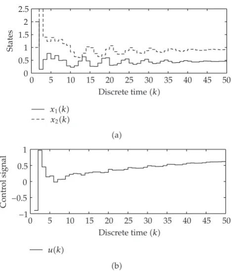
Figure 2:State trajectories and control signal versus time.
guarantees that the closed-loop systems trajectory is ultimately bounded and remains in the nonnegative orthant of the state space for nonnegative initial conditions. Witha 0.9,b 1,
σ1x, z 1/1e−cx1, . . . ,1/1e−6cx1,1/1e−cx2, . . . ,1/1e−6cx2T, c 0.5, q1 0.1,
γ1 0.1, and initial conditionsx0 2,1T andW0 0, . . . ,0T ∈ R12,Figure 2shows the
state trajectories versus time and the control signal versus time.
5. Neuroadaptive control for discrete-time nonlinear nonnegative uncertain systems with nonnegative control
As discussed in the introduction, control source inputs of drug delivery systems for physiological and pharmacological processes are usually constrained to be nonnegative as are the system states. Hence, in this section we develop neuroadaptive control laws for discrete-time nonnegative systems with nonnegative control inputs. In general, unlike linear nonnegative systems with asymptotically stable plant dynamics, a given set pointxe ∈Rn for a discrete-time nonlinear nonnegative dynamical system
xk1 fxkuk, x0 x0, k∈Z, 5.1
where xk ∈ Rn, uk ∈ Rn, andf : Rn → Rn, may not be asymptotically stabilizable with a constant control uk ≡ ue ∈ R
n
. Hence, we assume that the set point xe ∈ Rn satisfying
also asymptotically stable for allx0 ∈R
In this section, we assume that A in 4.4 is nonnegative and asymptotically stable, and hence, without loss of generality see 19, Proposition 3.1, we can assume that A
is an asymptotically stable compartmental matrix 19. Furthermore, we assume that the control inputs are injected directly into m separate compartments so that Bu and Gnx, z
in 4.14 are such that Bu diagb1, . . . , bnx is a positive diagonal matrix and Gnx, z diagonal matrix function. For compartmental systems, this assumption is not restrictive since control inputs correspond to control inflows to each individual compartment. For the statement of the next theorem, recall the definitions ofW andWk,k∈Z, given inTheorem 4.1. Theorem 5.1. Consider the discrete-time nonlinear uncertain dynamical systemGgiven by4.1and
4.2, where fx·,· and G·,· are given by 4.4 and 4.14, respectively, A is nonnegative and Then the neuroadaptive feedback control law
uik max
μ1 λminR/λmaxP, μ2 λmaxATP A/λminP, ξ max{b1q1s1, . . . , bnxqnxsnx}, ζ
min{q1, . . . , qnx}, andaandcare positive constants satisfyinga <1−γξandcμ2 < μ1. Furthermore,
uk≥≥0,xk≥≥0, andzk≥≥0,k∈Z, for allx0, z0∈R nx
×R
nz
.
Proof. SeeAppendix B.
6. Conclusion
In this paper, we developed a neuroadaptive control framework for adaptive set-point regulation of discrete-time nonlinear uncertain nonnegative and compartmental systems. Using Lyapunov methods, the proposed framework was shown to guarantee ultimate boundedness of the error signals corresponding to the physical system states and the neural network weighting gains while additionally guaranteeing the nonnegativity of the closed-loop system states associated with the plant dynamics.
Appendices
A. Proof ofTheorem 4.1
In this appendix, we proveTheorem 4.1. First, note that withuk,k ∈Z, given by4.15, it follows from4.1,4.4, and4.14that
xk1 Axk Δfxk, zkBuKxk−xe−BuWTkσ
xk, zk,Wk, x0 x0, k∈Z.
A.1
Now, definingexkxk−xeandezkzk−ze, using4.5–4.7,4.9, andAs ABuK,
it follows from4.2andA.1that
exk1 Asexk A−Ixe Δf
xk, zk−BuWTkσ
xk, zk,Wk
Asexk Bu
δxk, zk−δxe, ze
−Gn
xe, ze
ue−WTkσ
xk, zk
BuWTk
σxk, zk−σxk, zk,Wk
Asexk Bu
WTσxk, zkεxk, zk−WTkσxk, zk
BuWTk
σxk, zk−σxk, zk,Wk
Asexk−BuWTkσ
xk, zk,Wk
Bu
εxk, zk−WTσxk, zk,Wk
Asexk−BuWTkσ
xk, zk,WkBurk, ex0 x0−xe, k ∈Z,
A.2
ezk1 fz
exk, ezk
, ez0 z0−ze, A.3
where fzex, ez fzex xe, ez ze, εx, z ε1x, z, . . . , εnxx, z
T, σx, z
σT
1x, z, . . . , σnTxx, z
T
,WkWk−W,σx, z,Wσx, z,W−σx, z, andrεx, z− WTσx, z,Wi r1, . . . , rnx
T. Furthermore, sinceA
it follows fromTheorem 2.3that there exist a positivediagonalmatrixP diagp1, . . . , pnxand
a positive-definite matrixR∈Rnx×nxsuch that4.18holds.
Next, to show that the closed-loop system given by4.17,A.2, andA.3is ultimately bounded with respect toW, consider the Lyapunov-like function
Hence,
Furthermore, it follows fromA.12that
globally ultimately bounded with respect toWuniformly inex0, ez0with ultimate bound given by√ηw, whereηw>2ζαaβ/2aζ.
Next, to show ultimate boundedness of the error dynamics, consider the Lyapunov-like function
Note thatA.18satisfies
where inA.20we used lna−lnb lna/band ln1c≤ cfora, b >0 andc >−1. Now, notinga <2−ξandcμ2< μ1, using the inequalities
μ1P1/2ex2≤R1/2ex2,
2eTxATsPe≤cμ2P1/2ex2c−1P1/2e2,
A.21
and rearranging terms inA.20yields
Figure 3:Visualization of sets used in the proof ofTheorem 4.1.
which implies thatx1K∗ ≤α−1η. Next, letδ∈αx, γ, whereγ sup{r >0 :Bα−1βr0⊂
De}and assumex10 ∈ Bδ0andx1K > αx. Now, for everyk > 0 such thatx1k ≥αx,
k∈ {0, . . . ,k}, it follows that
αx1k≤αxT1k, xT2k
T
≤Ve
x1k, x2k, x3k
≤Ve
x10, x20, x30
≤βx10T, xT20T
≤β#δ2ε w
,
A.29
which implies thatx1k ≤α−1β
$ δ2ε
w,k∈ {0, . . . ,k}. Now, if there existsK∗>0 such
thatx1K∗ ≤ αx, then it follows as in the earlier case shown above thatx1k ≤ α−1η,
k≥K∗. Hence, ifx10∈ Bδ0, then
x1k≤α−1max%η, β#δ2ε w
&
εe, k∈Z. A.30
Finally, repeating the above arguments withx2k2≤εw,k∈Z, replaced byx2k2≤ηw,
k≥K >0, it can be shown thatx1k< ε,k≥K, whereε
√
eη−1. Next, define
Dα
ex, ez,W
∈Rnx×Rnz ×Rnx×s :V
e
ex, ez,W
≤α, A.31
whereαis the maximum value such thatDα⊆De, and define
Dη
ex, ez,W
∈Rnx×Rnz ×Rnx×s :V
e
ex, ez,W
≤εe2, A.32
whereεeis given byA.30. Assume thatD η ⊂DαseeFigure 3 this assumption is standard in the neural network literature and ensures that in the error spaceDethere exists at least one
Lyapunov level set Dη ⊂ Dα. In the case where the neural network approximation holds in
Rnx×Rnz, this assumption is automatically satisfied. SeeRemark A.1for further details. Now,
for allex, ez,W∈Dη∩De\Der,ΔVeex, ez,W≤0. Alternatively, for allex, ez,W∈Dη∩
Der,Veex, ez,W ΔVeex, ez,W≤ η ≤ εe2. Hence, it follows thatDη is positively invariant. In addition, since A.3 is input-to-state stable with ex viewed as the input, it follows from
Proposition 3.4 that the solutionezk, k ∈ Z, toA.3is ultimately bounded. Furthermore, it follows from 21, Theorem 1that there exist a continuous, radially unbounded, positive-definite function Vz : Rnz → R, a class-K∞ functionγ1·, and a class-K functionγ2·such
that
ΔVz
ez
≤ −γ1ezγ2ex. A.33
Since the upper bound forex2is given byeη−1/λminP, it follows that the set is given by
Dz
z∈ Dcz :Vz
z−ze
≤ max
z−ze γ1−1γ2
√ eη−1/λ
minP1/2
Vzz−ze
is also positively invariant as long as Dz ⊂ Dcz seeRemark A.1. Now, sinceD η andDz are positively invariant, it follows that
Dα
x, z,W∈Rnx×Rnz×Rnx×s :x−x
e, z−ze,W−W
∈D η, z∈ Dz
A.35
is also positively invariant. In addition, since 4.1, 4.2, 4.15, and 4.17 are ultimately bounded with respect tox,W; and since4.2is input-to-state stable atzk≡zewithxk−
xeviewed as the input then it follows fromProposition 3.4that the solutionxk, zk,Wk,
k ∈ Z, of the closed-loop system4.1,4.2,4.15, and4.17is ultimately bounded for all
x0, z0,W0∈ Dα.
Finally, to show thatxk≥≥ 0 andzk ≥≥ 0, k ∈ Z, for allx0, z0 ∈ R nx
×R
nz
note
that the closed-loop system4.1,4.15, and4.17, is given by
xk1 fx
xk, zkBuK
xk−xe
−BuWTkσ
xk, zk,Wk
ABuK
xk Δfxk, zk−BuWTkσ
xk, zk,Wk−BuKxe
fk, xk, zkv, x0 x0, k∈Z,
A.36
where
fk, x, zABuK
x Δfx, z−BuWTkσx, z,W, v−BuKxe. A.37
Note thatABuKandΔf·,·are nonnegative and, sinceσijx, z,Wi 0 wheneverWij>0,
i 1, . . . , nx, j 1, . . . , si, −WTσx, z,W ≥≥ 0. Hence, since fk, x, z is nonnegative with respect toxpointwise-in-time,fzx, zis nonnegative with respect toz, andv ≥≥0, it follows fromProposition 2.9thatxk≥≥0,k∈Z, andzk≥≥0,k ∈Z, for allx0, z0∈R
nx
×R nz
.
Remark A.1. In the case where the neural network approximation holds in Rnx × Rnz, the
assumptions Dη ⊂ Dα and Dz ⊂ Dcz invoked in the proof ofTheorem 4.1are automatically satisfied. Furthermore, in this case the control law4.15ensures global ultimate boundedness of the error signals. However, the existence of a global neural network approximator for an uncertain nonlinear map cannot in general be established. Hence, as is common in the neural network literature, for a given arbitrarily large compact set Dcx × Dcz ⊂ Rnx ×Rnz, we assume that there exists an approximator for the unknown nonlinear map up to a desired accuracy. Furthermore, we assume that in the error spaceDethere exists at least one Lyapunov
level set such that D η ⊂ Dα. In the case where δ·,· is continuous onRnx ×Rnz, it follows from the Stone-Weierstrass theorem thatδ·,·can be approximated over an arbitrarily large compact setDcx×Dcz. In this case, our neuroadaptive controller guarantees semiglobal ultimate boundedness. An identical assumption is made in the proof ofTheorem 5.1.
B. Proof ofTheorem 5.1
In this appendix, we proveTheorem 5.1. First, defineWukblock-diagWu1k, . . . ,Wu2k,
where
Wuik
⎧ ⎨ ⎩
0, if uik<0,
Wik, otherwise,
Next, note that withuk,k∈Z, given by5.2, it follows from4.1,4.4, and4.14that
xk1 Axk Δfxk, zk−BuWuTkσ
xk, zk, x0 x0, k∈Z. B.2
Now, definingexkxk−xeandezkzk−zeand using4.6,4.7, and4.9, it follows
from4.2andB.2that
exk1 Aexk A−Ixe Δf
xk, zk−BuWuTkσ
xk, zk
Aexk Bu
δxk, zk−δxe, ze
−Gn
xe, ze
ue−WTkσ
xk, zk
BuWk−Wuk
T
σxk, zk
Aexk−BuWTkσ
xk, zkBuε
xk, zk
BuWk−Wuk
T
σxk, zk, ex0 x0−xe, k ∈Z,
B.3
ezk1 fz
exk, ezk
, ez0 z0−ze, B.4
where fzex, ez fzex xe, ez ze, and εx, z ε1x, z, . . . , εnxx, z
T. Furthermore,
sinceAis nonnegative and asymptotically stable, it follows fromTheorem 2.3that there exist a positivediagonalmatrixP diagp1, . . . , pnxand a positive-definite matrixR∈R
nx×nx such
that5.5holds.
Next, to show ultimate boundedness of the closed-loop system5.4, B.3, andB.4, consider the Lyapunov-like function
Vwex, ez,W trWQ −1WT, B.5
whereQdiagq1, . . . ,qnx diagq1/p1b1, . . . , qnx/pnxbnxandWkWk−W withW
block-diagW1, . . . , Wnx. Note that B.5 satisfies 3.3 with x1 q
−1/2
1 W1T, . . . ,q−1 /2 nx W
T nx
T,
x2 eTx, eTz T
,αx1 βx1 x12, wherex12 trWQ −1WT. Furthermore,αx1is
a class-K∞function. Now, using5.4andB.3, it follows that the difference ofVwex, ez,W along the closed-loop system trajectories is given by
ΔVw
exk, ezk,Wk
trWk1Q−1WTk1−trWkQ−1WTk
nx
i 1
2pibiP1/2exk 1P1/2e
xk2
γeikσi
xk, zk−Wik
T
Wik
nx
i 1
pibiqiP1/2exk2
1P1/2e xk2
2γeikσi
nx
B.6gives the following:
2otherwise,Wuik Wik, and hence, usingA.8,A.9,B.7, B.9, andB.10, it
Hence, it follows fromB.6that in either case
ΔVw
Now, it follows using similar arguments as in the proof ofTheorem 4.1that the closed-loop system 5.4, B.3, and B.4 is globally bounded with respect to W uniformly in
using similar arguments as in the proof ofTheorem 4.1that the closed-loop system5.4,B.3, and B.4is globally ultimately bounded with respect to W uniformly in ex0, ez0 with ultimate bound given by√ηw, whereηw>2ζαγaβ/2aζ. Alternatively, if there exists
k∗∈Zsuch thatexk 0 for allk≥k∗, thenWk Wk∗for allk≥k∗.
Next, usingA.21andB.17yields Now, using similar arguments as in the proof of Theorem 4.1 it follows that the solution
xk, zk,Wk, k ∈ Z, of the closed-loop system 5.4, B.3, and B.4 is ultimately
References
1T. Hayakawa, W. M. Haddad, J. M. Bailey, and N. Hovakimyan, “Passivity-based neural network adaptive output feedback control for nonlinear nonnegative dynamical systems,”IEEE Transactions on Neural Networks, vol. 16, no. 2, pp. 387–398, 2005.
2T. Hayakawa, W. M. Haddad, N. Hovakimyan, and V. Chellaboina, “Neural network adaptive control for nonlinear nonnegative dynamical systems,”IEEE Transactions on Neural Networks, vol. 16, no. 2, pp. 399–413, 2005.
3A. Berman and R. J. Plemmons,Nonnegative Matrices in the Mathematical Sciences, Academic Press, New York, NY, USA, 1979.
4A. Berman, M. Neumann, and R. J. Stern,Nonnegative Matrices in Dynamic Systems, Pure and Applied Mathematics, John Wiley & Sons, New York, NY, USA, 1989.
5L. Farina and S. Rinaldi,Positive Linear Systems: Theory and Application, Pure and Applied Mathematics, John Wiley & Sons, New York, NY, USA, 2000.
6E. Kaszkurewicz and A. Bhaya, Matrix Diagonal Stability in Systems and Computation, Birkh¨auser, Boston, Mass, USA, 2000.
7T. Kaczorek,Positive 1D and 2D Systems, Springer, London, UK, 2002.
8W. M. Haddad and V. Chellaboina, “Stability and dissipativity theory for nonnegative dynamical systems: a unified analysis framework for biological and physiological systems,”Nonlinear Analysis: Real World Applications, vol. 6, no. 1, pp. 35–65, 2005.
9R. R. Mohler, “Biological modeling with variable compartmental structure,” IEEE Transactions on Automatic Control, vol. 19, no. 6, pp. 922–926, 1974.
10H. Maeda, S. Kodama, and F. Kajiya, “Compartmental system analysis: realization of a class of linear systems with physical constraints,”IEEE Transactions on Circuits and Systems, vol. 24, no. 1, pp. 8–14, 1977.
11I. W. Sandberg, “On the mathematical foundations of compartmental analysis in biology, medicine, and ecology,”IEEE Transactions on Circuits and Systems, vol. 25, no. 5, pp. 273–279, 1978.
12H. Maeda, S. Kodama, and Y. Ohta, “Asymptotic behavior of nonlinear compartmental systems: nonoscillation and stability,” IEEE Transactions on Circuits and Systems, vol. 25, no. 6, pp. 372–378, 1978.
13R. E. Funderlic and J. B. Mankin, “Solution of homogeneous systems of linear equations arising from compartmental models,”SIAM Journal on Scientific and Statistical Computing, vol. 2, no. 4, pp. 375–383, 1981.
14D. H. Anderson,Compartmental Modeling and Tracer Kinetics, vol. 50 ofLecture Notes in Biomathematics, Springer, Berlin, Germany, 1983.
15K. Godfrey,Compartmental Models and Their Application, Academic Press, London, UK, 1983.
16J. A. Jacquez,Compartmental Analysis in Biology and Medicine, University of Michigan Press, Ann Arbor, Mich, USA, 1985.
17D. S. Bernstein and D. C. Hyland, “Compartmental modeling and second-moment analysis of state space systems,”SIAM Journal on Matrix Analysis and Applications, vol. 14, no. 3, pp. 880–901, 1993. 18J. A. Jacquez and C. P. Simon, “Qualitative theory of compartmental systems,”SIAM Review, vol. 35,
no. 1, pp. 43–79, 1993.
19W. M. Haddad, V. Chellaboina, and E. August, “Stability and dissipativity theory for discrete-time non-negative and compartmental dynamical systems,”International Journal of Control, vol. 76, no. 18, pp. 1845–1861, 2003.
20W. M. Haddad and V. Chellaboina, Nonlinear Dynamical Systems and Control: A Lyapunov-Based Approach, Princeton University Press, Princeton, NJ, USA, 2008.
21Z.-P. Jiang and Y. Wang, “Input-to-state stability for discrete-time nonlinear systems,”Automatica, vol. 37, no. 6, pp. 857–869, 2001.
22H. L. Royden,Real Analysis, Macmillan, New York, NY, USA, 3rd edition, 1988.