R E S E A R C H
Open Access
Semi-nonoscillation intervals in the
analysis of sign constancy of Green’s
functions of Dirichlet, Neumann and focal
impulsive problems
Alexander Domoshnitsky
1*and Guy Landsman
2*Correspondence: [email protected] 1Department of Mathematics, Ariel University, Ariel, Israel
Full list of author information is available at the end of the article
Abstract
We consider the following second order differential equation with delay:
(Lx)(t)≡x(t) +pj=1aj(t)x(t–
τ
j(t)) +p
j=1bj(t)x(t–
θ
j(t)) =f(t), t∈[0,ω
],x(tk) =
γ
kx(tk– 0),x(tk) =δ
kx(tk– 0), k= 1, 2,. . .,r.In this paper we use focal problems to analyze the sign constancy of Green’s functions.
MSC: 34K10; 34B37; 34A40; 34A37; 34K48
Keywords: impulsive equations; Green’s functions; positivity/negativity of Green’s functions; boundary value problem; second order
1 Introduction
Impulsive equations attract attention of many recognized mathematicians. See, for ex-ample, the books [–]. The positivity of solutions to the Dirichlet problem was studied in []. A generalized Dirichlet problem was considered in [–]. Multipoint problems and problems with integral boundary conditions were considered in [–]. The Dirichlet problem for impulsive equations with impulses at variable moments was studied in []. All these works considered impulsive ordinary differential equations.
Let us assume that all trajectories of solutions to a non-impulsive ordinary differential equation are known. In this case, impulses imply only choosing the trajectory between the points of impulses, but we stay on the trajectory of a corresponding solution of the non-impulsive equation betweentiandti+. In the case of an impulsive equation with delay, it is not true anymore. That is why the properties of delay impulsive equations can be quite different.
There are only a few results on the positivity of solutions to impulsive differential equa-tions with delay. Note the results [–] about the positivity of Green’s funcequa-tions for boundary value problems for first order delay impulsive equations. Nonoscillation of sec-ond order delay impulsive differential equation was studied in []. Sturmian comparison
theory for impulsive second order delay equations was studied in []. The positivity of Green’s functions for the nth order impulsive delay differential equation was considered in []. The idea of construction of Green’s functions for second order impulsive differential equations was first proposed in []. The use of Green’s functions for auxiliary impul-sive problems in the study of sign constancy of delay impulimpul-sive differential equations was proposed in [], where a one-point problem was studied. Note also paper [] for focal problems.
In this paper we use the results for one-point and focal problems in order to obtain results on the sign constancy for Green’s functions of two-point boundary value problems.
Let us consider the following impulsive equations:
(Lx)(t)≡x(t) + p
j=
aj(t)x
t–τj(t)
+ p
j=
bj(t)x
t–θj(t)
=f(t), t∈[,ω] (.)
x(tk) =γkx(tk– ), x(tk) =δkx(tk– ), k= , , . . . ,r, (.)
=t<t<t<· · ·<tr<tr+=ω,
x(ζ) = , ζ< , (.)
wheref,aj,bj: [,ω]→Rare summable functions andτj,θj: [,ω]→[, +∞) are mea-surable functions forj= , , . . . ,p.pandrare natural numbers,γkandδkare real positive numbers.
LetDbe a space of functionsx: [,ω]→Rsuch that their derivativex(t) is absolutely continuous on every intervalt∈[ti,ti+),i= , . . . ,r,x∈L∞, there exist the finite limits
x(ti– ) =limt→t–
i x(t) andx
(t
i– ) =limt→t– i x
(t) and condition (.) is satisfied at points
ti(i= , . . . ,r). We understand solutionxas a functionx∈Dsatisfying (.)-(.).
Definition . We call [,ω] a semi-nonoscillation interval of (Lx)(t) = if every nontriv-ial solution having zero of derivative does not have zero on this interval.
The influence of nonoscillation on sign properties of Green’s functions in the case of nth order differential equations was found in the known papers [, ]. An extension of these results on delay differential equations was obtained in [, ]. The importance of a semi-nonoscillation interval in the case of non-impulsive delay differential equations was first noted in []. In this paper we develop the use of semi-nonoscillation intervals to impulsive delay differential equations.
2 Construction of Green’s functions
For equation (.) we consider the following variants of boundary conditions:
x(ω) = , x(ω) = , (.)
x() = , x(ω) = , (.)
x() = , x(ω) = , (.)
x() = , x(ω) = , (.)
Thus boundary conditions (.), (.), (.) are of focal sort, (.) is Dirichlet’s one, (.) is Neumann’s condition.
We denote byGi(t,s) Green’s function of problem (.)-(.), (.i) respectively.
It is known from the formula of solutions’ representation for a system of delay impulsive equations (see [] and []) that the general solution of (.)-(.) can be represented in the form
x(t) =v(t)x() +C(t, )x() + t
C(t,s)f(s)ds, (.)
where C(t,s) is the Cauchy function andv(t) is the solution of the semi-homogenous problem
⎧ ⎨ ⎩
(Lx)(t) = , t∈[,ω],
x() = , x() = . (.)
C(t,s), as a function oft, for every fixeds, satisfies the equation
x(t) + p
j=
aj(t)x
t–τj(t)
+ p
j=
bj(t)x
t–θj(t)
= , t∈[s,ω], (.)
x(tk) =γkx(tk– ), x(tk) =δkx(tk– ), k=is+ , . . . ,r, (.)
tis<s<tis+<· · ·<tr<tr+=ω,
x(ζ) =x(ζ) = , ζ<s, (.)
and the initial conditionsC(s,s) = ,∂∂tC(s,s) = . Note thatC(t,s) = fort<s.
Using this general representation, we can obtain the following formulas of Green’s func-tions:
G(t,s) =C(t,s) +
h(t,s)
v(ω)Ct(ω, ) –v(ω)C(ω, )
, (.)
where
h(t,s) =Ct(ω,s)v(t)C(ω, ) –v(ω)C(t, )
+C(ω,s)v(ω)C(t, ) –v(t)Ct(ω, )
,
G(t,s) =C(t,s) –C(t, )
Ct(ω,s)
Ct(ω, )
, (.)
G(t,s) =C(t,s) –C(ω,s)
v(t)
v(ω)
, (.)
G(t,s) =C(t,s) –C(t, )
C(ω,s)
C(ω, ). (.)
Let us consider the following homogeneous equation:
Lemma . If
() bj(t)≤,t∈[,ω];
() the Cauchy functionC(t,s)of the first order equation
⎧ ⎪ ⎪ ⎨ ⎪ ⎪ ⎩
y(t) +pj=aj(t)y(t–τj(t)) = , t∈[,ω],
y(tk) =δky(tk– ), k= , . . . ,m,
y(ζ) = , ζ< ,
(.)
is positive for≤s≤t≤ω.
Then the Cauchy function C(t,s)of equation(.)and its derivative Ct(t,s)are positive in≤s≤t≤ω.
Proof It follows from the conditionC(s,s) = ,C(s,s) = that there exists s> such that
C(t,s) > andCt(t,s) > fort∈(s,s+ s). Let us suppose that there exists a pointηsuch thatCt(η,s) = ,Ct(t,s) > fort∈[,η). It is clear that in this casex(t) =C(t,s) satisfies the equation
x(t) + p
j=
aj(t)x
t–τj(t)
=φ(t), t∈[s,ω], (.)
whereφ(t) = –pj=bj(t)x(t–θj(t)),t∈[s,η]. It follows from the nonnegativity ofbj(t) (j= , . . . ,p) and the positivity ofx(t) =C(t,s) thatφ(t)≥ fort∈[,η].
Let us denotey(t) =x(t). Then we can write an equation fory(t) in the form
⎧ ⎪ ⎪ ⎨ ⎪ ⎪ ⎩
y(t) +pj=aj(t)y(t–τj(t)) =φ(t), t∈[s,ω],
y(tk) =δky(tk– ), k= , . . . ,m,
y(ζ) = , ζ< .
(.)
It is clear thaty(s) = . The solution of (.) can be written
y(t) = t
s
C(t,ζ)φ(ζ)dζ+C(t,s), (.)
whereC(t,s) is the Cauchy function of (.). Now it is clear that
y(η) = η
s
C(η,ζ)φ(ζ)dζ+C(η,s) > . (.)
Lemma . has been proven.
Lemma . If the conditions()and()of Lemma.are fulfilled,then Green’s function
G(t,s)of (.)-(.), (.)exists and there exists an interval(, s)such that G(t,s) < for
t∈(, s).
It is clear that
G(,s) =C(,s) –C(, )
Ct(ω,s)
Ct(ω, )
= , (.)
Gt(,s) = –Ct(, )C t(ω,s)
Ct(ω, ) = –
Ct(ω,s)
Ct(ω, )< . (.)
It means from (.) that there exists an interval (, s) such thatG(t,s) < fort∈(, s).
Lemma . has been proven.
Lemma . If the conditions()and()of Lemma.are fulfilled,then Green’s function G(t,s)of (.)-(.), (.)exists and there exists an interval(, s)such that G(t,s) < for
t∈(, s).
Proof It follows from the conditionv() = ,v() = , wherev(t) is a solution of problem (.), that there exists > such thatv(t) > fort∈(, ). Let us suppose that there exists a pointηsuch thatv(η) = ,v(t) > fort∈[,η). It is clear that in this casex(t) =v(t) satisfies the equation
x(t) + p
j=
aj(t)x
t–τj(t)
=φ(t), t∈[s,ω], (.)
whereφ(t) = –pj=bj(t)x(t–θj(t)),t∈[s,η]. It follows from the nonnegativity ofbj(t) (j= , . . . ,p) and the positivity ofx(t) =v(t) thatφ(t)≥ fort∈[,η].
Let us denotey(t) =x(t). Then we can write an equation fory(t) in the form
⎧ ⎪ ⎪ ⎨ ⎪ ⎪ ⎩
y(t) +pj=aj(t)y(t–τj(t)) =φ(t), t∈[s,ω],
y(tk) =δky(tk– ), k= , . . . ,m,
y(ζ) = , ζ< .
(.)
It is clear thaty(s) = . The solution of (.) can be written
y(t) = t
s
C(t,ζ)φ(ζ)dζ, (.)
whereC(t,s) is the Cauchy function of (.). Now, from the positivity ofC(t,ζ), it is clear that
y(η) = η
s
C(η,ζ)φ(ζ)dζ> . (.)
It means thatv(η) =y(η) > . Now it is clear thatv(t) > fort∈[,ω]. It means that there is no nontrivial solution to the problem (Lx)(t) = ,x() = ,x(ω) = . If there is no nontrivial solution of the problem, then Green’s function of (.)-(.), (.) exists and
G(,s) =C(,s) –C(ω,s)
v()
v(ω)
= –C(ω,s)
v(ω)
< . (.)
Lemma . If the conditions()and()of Lemma.are fulfilled,then Green’s function G(t,s)of (.)-(.), (.)exists and there exists an interval(, s)such that G(t,s) < for
t∈(, s).
Proof Let us demonstrate that the problem (Lx)(t) = ,x() = ,x(ω) = has only the triv-ial solution. If there exists a nontrivtriv-ial solution of this problem, it is proportional toC(t, ). According to Lemma .,C(t, ) > fort∈(,ω]. It means thatx(ω) =C(ω, ) > . That contradicts the assumptionx(ω) = .
Let us take a look atG(,s) andGt(,s)
G(,s) = –C(, )
C(ω,s)
C(ω, )= , (.)
Gt(,s) = –Ct(, )C(ω,s)
C(ω, )= –
C(ω,s)
C(ω, )< , (.)
sinceC(t,s) is positive. It means that there exists an interval (, s) such thatG(t,s) < fort∈(, s).
Lemma . has been proven.
3 Sign constancy of Green’s functions
In this section we will prove the sign constancy of Green’s functionsG(t,s) andG(t,s) using the results from [] and [] about the sign constancy ofG(t,s),G(t,s) andG(t,s).
Theorem . Assume that the following conditions are fulfilled:
() Gξ(t,s)≥,t,s∈[,ξ]for every <ξ<ω.
() [,ω]is a semi-nonoscillation interval of(Lx)(t) = . () bj(t)≤,t∈[,ω].
() The Cauchy functionC(t,s)of the first order equation(.)is positive for ≤s≤t≤ω.
Then G(t,s)≤,G(t,s)≤,G(t,s)≤for t,s∈[,ω]and under the additional
con-ditionpj=bj(t)χ(t–θj(t)) ≡,t∈[,ω],where
χ(t,s) = ⎧ ⎨ ⎩
, t≥s,
, t<s, (.)
we have also G(t,s)≤for t,s∈[,ω].
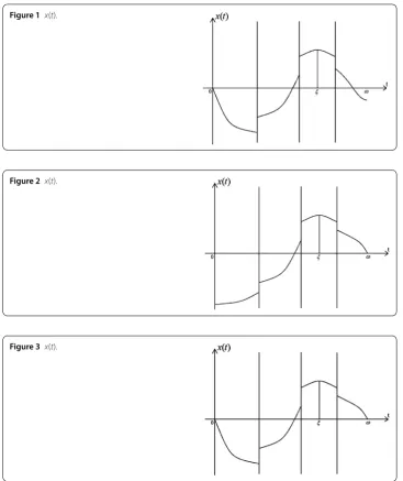
Proof Let us start with problem (.)-(.), (.). According to Lemma ., there exists a unique solution for every summablef(t). Let us assume thatG(t,s) changes sign. It means that there exists a functionf(t)≥ such that the solutionx(t) changes sign. Then there is a point <ξ<ωsuch thatx(ξ) > andx(ξ) = (see Figure ). From condition , we know that Green’s function for this problemGξ(t,s) is nonnegative. Thenx(t)≥ for
t∈[,ξ]. But, according to Lemma .,x(t) < fortwhich are close to . This contraction demonstrates that the solutionx(t) cannot change its sign for nonnegativef(t). This proves thatG(t,s) should be nonpositive.
Figure 1 x(t).
Figure 2 x(t).
Figure 3 x(t).
that there exists a functionf(t)≥ such that the solutionx(t) changes sign. Then there is a point <ξ<ωsuch thatx(ξ) > andx(ξ) = (see Figure ). From condition , we know that Green’s function for this problemGξ(t,s) is nonnegative. Thenx(t)≥ fort∈
[,ξ]. But, according to Lemma .,x(t) < fortwhich are close to . This contraction demonstrates that the solutionx(t) cannot change its sign for nonnegativef(t). This proves thatG(t,s) should be nonpositive.
Let us now consider problem (.)-(.), (.). According to Lemma ., there exists a unique solution for every summable f(t). Let us assume thatG(t,s) changes sign. It means that there exists a functionf(t)≥ such that the solutionx(t) changes sign. Then there is a point <ξ<ωsuch thatx(ξ) > andx(ξ) = (see Figure ). From condition , we know that Green’s function for this problemGξ(t,s) is nonnegative. Thenx(t)≥ for
Let us now consider problem (.)-(.), (.). The condition
p
j=
bj(t)χ
t–θj(t)
≡ (.)
means thatbj(t)χ(t–θj(t)) < on the set of positive measure. Let us prove the nonpositivity of Green’s functionG(t,s) step by step.
Step . Let us suppose that there is a solution of (Lx)(t) =f(t),t∈[,ω],x() =x(ω) = with nonnegativef(t)≥,f(t) ≡ such thatx(t)≥. It is clear that thisx(t) satisfies the equation
x(t) + p
j=
aj(t)x
t–τj(t)
=φ(t), t∈[,ω], (.)
where φ(t) = f(t) –pj=bj(t)x(t–θj(t)). It is clear that φ(t)≥ and from the fact p
j=bj(t)χ(t–θj(t)) < on the set of positive measure, we haveφ(t) > fort∈[,ω]. Let us denotey(t) =x(t). Then we can write an equation fory(t) in the form
⎧ ⎨ ⎩
y(t) +pj=aj(t)y(t–τj(t)) =φ(t), t∈[,ω],
y(ζ) = , ζ< . (.)
It is clear thaty() = . The solution of (.) can be written
y(t) = t
C(t,s)φ(s)ds, (.)
whereC(t,s) is the Cauchy function of (.). It follows thatC(t,s) > from []. Now it is clear that
y(ω) = ω
C(t,s)φ(s)ds> , (.)
andx(ω) =y(ω) > . This demonstrates that the casex(t) > forf(t)≥,f(t) ≡ is im-possible.
Step . Let us assume that there exists a solutionx(t) changing sign on [,ω] for non-negativef(t). We have to consider two cases: the solutionx(t) changes sign first time from positive to negative; and the solutionx(t) changes sign first from negative to positive.
In the first case, we have a pointηsuch thatx(η) = . It means that our functionx(t) satisfies the problem (Lx)(t) =f(t),x() = ,x(η) = . We have proven above thatG(t,s)≤ and this excludes the possibility ofx(t) > fort∈[,η).
In the second case, we have a pointξsuch that ⎧
⎨ ⎩
(Lx)(t) =f(t), t∈[,ω],
x(ξ) =α> , x(ξ) = , (.)
and the conditionGξ(t,s)≥ implies thatx(t) > . We proved in Step that the situation
x(t) > is impossible. ThenG(t,s)≤ fort,s∈[,ω].
Theorem . Assume that aj≥,bj≤for j= , . . . ,p, <γk≤, <δk≤for k= , . . . ,r,
and there exists a function v∈D and > such that
(Lv)(t)≥ > , v(t) > , v(t) < , v(t) > , t∈(,ω), (.)
where the differential operator L is defined by(.).And let[,ω]be a semi-nonoscillation interval of (Lx)(t) = . Then Green’s functions G(t,s), G(t,s), G(t,s) satisfy the
in-equalities G(t,s) ≤ ,G(t,s) ≤ ,G(t,s) ≤ , (t,s) ∈ [,ω]×[,ω]. If, in addition, p
j=bj(t)χ(t–θj(t)) ≡,t∈[,ω],then G(t,s)≤, (t,s)∈[,ω]×[,ω].
Proof It is clear that all the conditions of assertion () of Theorem . from [] are ful-filled. According to this theorem,Gξ(t,s)≥ for everyt,s∈(,ω) and every <ξ<ω. Us-ing Theorem . above, we obtain thatG(t,s)≤,G(t,s)≤,G(t,s)≤ fort,s∈[,ω]. If, in addition, pj=bj(t)χ(t–θj(t)) ≡,t ∈[,ω], then it follows that G(t,s)≤ for
t,s∈[,ω].
Theorem . has been proven.
Theorem . Assume that the following conditions are fulfilled:
() Gξ(t,s)≤,t,s∈[,ξ]for every <ξ<ω.
() [,ω]is a semi-nonoscillation interval of(Lx)(t) = . Then G(t,s)≤for t,s∈[,ω].
Proof Let us consider problem (.)-(.), (.). According to Lemma ., there exists a unique solution for every summablef(t). Let us assume thatG(t,s) changes sign. It means that there exists a functionf(t)≥ such that the solutionx(t) changes sign from negative to positive according to Lemma .. Then there is a point <ξ<ωsuch thatx(ξ) =α> andx(ξ) = (see Figure ). From condition , we know that Green’s function for this problem,Gξ(t,s) is nonpositive. From condition , it follows that the solution of problem (Lx)(t) = ,x(ξ) =α> ,x(ξ) = is positive fort∈(,ξ]. Thenx(t)≤ fort∈[,ξ]. This contradicts Lemma ., which claims thatx(t) can change its sign only from negative to positive for nonnegativef(t). ThenG(t,s) should be nonpositive.
Theorem . has been proven.
Theorem . Assume that aj≥,bj≥for j= , . . . ,p, ≤γk, ≤δk,for k= , . . . ,r,and
there exists a function v∈D and > such that
(Lv)(t)≤– < , v(t) > , v(t) > , v(t) < , t∈(,ω), (.)
where the differential operator L is defined by(.).And let[,ω]be a semi-nonoscillation interval of (Lx)(t) = .Then Green’s function G(t,s)of (.)-(.), (.)satisfies the
in-equality G(t,s)≤, (t,s)∈[,ω]×[,ω].
Proof Looking at Theorem . from [], we can see that the problem satisfies all of the conditions. ThenG(t,s)≤ for everyt,s∈(,ω). Using Theorem . above, we obtain thatG(t,s)≤ fort,s∈[,ω].
Example . Let us now find an example of a functionvsatisfying the condition of The-orem .. To this end, let us start withv(t) =e–αtin the intervalt∈[,t
). The functionv in the rest of the intervals will be of the form
v(t) =cie–αait, t∈[ti,ti+), (.)
After some calculations, we get thatvis of the form
⎧
For the next theorems, we use the following notation:
E= min
Proof Let us substitute thisv(t), defined by (.), into the condition of Theorem .
whereis defined by (.). DenotingF(α) =αEe–αE, we can find its maximum using
the derivative
F(α) =αe–αE–αEe–αEE=α( –Eα)e–αEE, (.)
and we get thatα=Eis a point of maximum. Substituting thisαinto (.), we see that (.) implies, according to Theorem ., the nonnegativity ofP(t,s).
Theorem . has been proven.
In the particular caseaj(t) = ,j= , . . . ,p, we have
Proof Let us substitute thisv(t), defined by (.), into the condition of Theorem .
α(
Theorem . Assume that
Then[,ω]is a semi-nonoscillation interval.
Example . Let us now find an example of a functionvsatisfying the condition of
The-orem .. To this end, let us start withv(t) =t(ω–t) in the intervalt∈[,t), where is a small positive constant. The functionvin the rest of the intervals will be of the form
v(t) =v(ti) +v(ti)(t–ti) – (t–ti), t∈[ti,ti+),i= , . . . ,r,tr+=ω, (.) For the next corollary, we use the following notation:
Proof Let us substitute thisv(t), defined by (.), into the assertion of Theorem .
The authors declare that they have no competing interests.
Authors’ contributions
All authors contributed equally to the writing of this paper. All authors read and approved the final manuscript.
Author details
1Department of Mathematics, Ariel University, Ariel, Israel.2Department of Mathematics, Bar Ilan University, Ramat Gan, Israel.
Acknowledgements
Dr. Shlomo Yanetz (Bar Ilan University, Israel) for his important and valuable remarks. This paper is a part of the second author’s Ph.D. thesis which is being carried out in the Department of Mathematics at Bar-Ilan University.
Publisher’s Note
Springer Nature remains neutral with regard to jurisdictional claims in published maps and institutional affiliations.
Received: 1 December 2016 Accepted: 9 March 2017 References
1. Azbelev, NV, Maksimov, VP, Rakhmatullina, LF: Introduction to the Theory of Linear Functional-Differential Equations. Advanced Series in Math. Science and Engineering, vol. 3. World Federation Publisher Company, Atlanta (1995) 2. Bainov, D, Simeonov, P: Impulsive Differential Equations. Pitman Monographs and Surveys in Pure and Applied
Mathematics, vol. 66. Longman Scientific, Harlow (1993)
3. Lakshmikantham, V, Bainov, DD, Simeonov, PS: Theory of Impulsive Differential Equations. World Scientific, Singapore (1989)
4. Pandit, SG, Deo, SG: Differential Equations Involving Impulses. Lecture Notes in Mathematics, vol. 954. Springer, Berlin (1982)
5. Samoilenko, AM, Perestyuk, AN: Impulsive Differential Equations. World Scientific, Singapore (1992)
6. Zavalishchin, SG, Sesekin, AN: Dynamic Impulse Systems: Theory and Applications. Mathematics and Its Applications, vol. 394. Kluwer, Dordrecht (1997)
7. Jiang, D, Lin, X: Multiple positive solutions of Dirichlet boundary value problems for second order impulsive differential equations. J. Math. Anal. Appl.321, 501-514 (2006)
8. Feng, M, Xie, D: Multiple positive solutions of multi-point boundary value problem for second-order impulsive differential equations. J. Comput. Appl. Math.223, 438-448 (2009)
9. Jiang, J, Liu, L, Wu, Y: Positive solutions for second order impulsive differential equations with Stieltjes integral boundary conditions. Adv. Differ. Equ.2012, 124 (2012)
10. Hao, X, Liu, L, Wu, Y: Positive solutions for second order impulsive differential equations with integral boundary conditions. Commun. Nonlinear Sci. Numer. Simul.16, 101-111 (2011)
11. Hu, L, Liu, L, Wu, Y: Positive solutions of nonlinear singular two-point boundary value problems for second-order impulsive differential equations. Appl. Math. Comput.196, 550-562 (2008)
12. Jankowski, T: Positive solutions to second order four-point boundary value problems for impulsive differential equations. Appl. Math. Comput.202, 550-561 (2008)
13. Jankowski, T: Positive solutions for second order impulsive differential equations involving Stieltjes integral conditions. Nonlinear Anal.74, 3775-3785 (2011)
14. Lee, EK, Lee, YH: Multiple positive solutions of singular two point boundary value problems for second order impulsive differential equations. Appl. Math. Comput.158, 745-759 (2004)
16. Rachunkova, I, Tomecek, J: A new approach to BVPs with state-dependent impulses. Bound. Value Probl.2013, 22 (2013). doi:10.1186/1687-2770-2013-22
17. Domoshnitsky, A, Drakhlin, M: Nonoscillation of first order impulse differential equations with delay. J. Math. Anal. Appl.206, 254-269 (1997)
18. Domoshnitsky, A, Volinsky, I: About positivity of Green’s functions for nonlocal boundary value problems with impulsive delay equations. Sci. World J.2014, Article ID 978519 (2014)
19. Domoshnitsky, A, Volinsky, I: About differential inequalities for nonlocal boundary value problems with impulsive delay equations. Math. Bohem.140, 121-128 (2015)
20. Tian, YL, Weng, PX, Yang, JJ: Nonoscillation for a second order linear delay differential equation with impulses. Acta Math. Appl. Sin.20, 101-114 (2004)
21. Bainov, D, Domshlak, Y, Simeonov, P: Sturmian comparison theory for impulsive differential inequalities and equations. Arch. Math.67, 35-49 (1996)
22. Domoshnitsky, A, Drakhlin, M, Litsyn, E: On boundary value problems for N-th order functional differential equations with impulses. Adv. Math. Sci. Appl.8(2), 987-996 (1998)
23. Domoshnitsky, A, Landsman, G, Yanetz, S: About sign-constancy of Green’s functions for impulsive second order delay equations. Opusc. Math.34(2), 339-362 (2014)
24. Domoshnitsky, A, Landsman, G, Yanetz, S: About sign-constancy of Green’s function of one-point problem for impulsive second order delay equations. Funct. Differ. Equ.21(1-2), 3-15 (2014)
25. Domoshnitsky, A, Landsman, G, Yanetz, S: About sign-constancy of Green’s function of a two-point problem for impulsive second order delay equations. Electron. J. Qual. Theory Differ. Equ.2016, 9 (2016)
26. Chichkin, EA: Theorem about differential inequality for multipoint boundary value problems. Izv. Vysš. Uˇcebn. Zaved., Mat.27(2), 170-179 (1962)
27. Levin, AY: Non-oscillation of solutions of the equationx(n)+p
n–1(t)x(n–1)+· · ·+p0(t)x= 0. Usp. Mat. Nauk24(2), 43-96 (1969)
28. Azbelev, NV, Domoshnitsky, A: A question concerning linear differential inequalities. Differ. Equ.27, 257-263 (1991); translation from Differentsial’nye uravnenija, 27, 257-263 (1991)
29. Azbelev, NV, Domoshnitsky, A: A question concerning linear differential inequalities. Differ. Equ.27, 923-931 (1991); translation from Differentsial’nye uravnenija, 27, 641-647 (1991)