FULL PAPER
Temporal change of near-surface
shear wave velocity associated with rainfall
in Northeast Honshu, Japan
Yu Miao, Yang Shi and Su‑Yang Wang
*Abstract
We apply seismic interferometry to earthquake records to investigate temporal change of near‑surface shear wave velocity associated with rainfall in Northeast Honshu, Japan. We observe there exists a threshold (around 100 mm of 24 h rainfall total) of the temporal influence of rainfall on near‑surface shear wave velocity. The velocity does not change significantly under low‑intensity rainfall, while it is reduced by 1–3% with one exception of 10% when the rainfall intensity exceeds the threshold. Compared with the travel time of no rain, the travel time increment of low‑ intensity rainfall is no more than 3 × 10⁻⁴ s, while that of high‑intensity rainfall ranges between 10−3 and 10−2 s. Based
on the results of observation, we propose a one‑dimensional model to compute the travel time increment, which can give a preliminary estimation of the temporal influence of rainfall on near‑surface shear wave velocity.
Keywords: Earthquake ground motions, Seismic interferometry, KiK‑net, Rainfall
© The Author(s) 2018. This article is distributed under the terms of the Creative Commons Attribution 4.0 International License (http://creat iveco mmons .org/licen ses/by/4.0/), which permits unrestricted use, distribution, and reproduction in any medium, provided you give appropriate credit to the original author(s) and the source, provide a link to the Creative Commons license, and indicate if changes were made.
Introduction
Near-surface shear wave velocity has been recognized as an important mechanical parameter in the fields of earth-quake engineering and geophysics. It has a wide range of application such as classifying site classes (Borcherdt 1994), evaluating liquefaction potential (Ahmadi and Paydar 2014) and estimating local site response (Choi and Stewart 2005) for seismic design of buildings, struc-tures, and underground utilities (Lee et al. 2014). And its relevance to evolving stress and effective rheology at depth for seismic monitoring of faults (Hillers and Campillo 2016; Wegler and Sens-Schönfelder 2010), vol-canoes (Brenguier et al. 2014; Wegler et al. 2006), land-slides (Mainsant et al. 2012; Pilz et al. 2014; Xu et al. 2017) and hydrocarbon reservoirs (Bakulin and Calvert 2006; Miyazawa et al. 2008) is well documented.
Hardin and Black (1968) expressed the shear wave modulus of soil as a function of eleven factors, mainly including effective stress, void ratio, saturation, strain history, temperature, grain properties and soil structure.
And the shear wave velocity of rock can be influenced by porosity, fluid saturation, fractures, pressure and tem-perature (Toksoz et al. 1976). Hence the near-surface shear wave velocity is subjected to a variety of environ-ment conditions, such as crustal stress, ground surface perturbation and atmospheric forcing. Many researchers have observed change of near-surface velocity caused by strong motion (Hobiger et al. 2012; Nakata and Snieder 2011; Niu et al. 2008), plate motion (Nakata and Snieder 2012a; Takagi and Okada 2012), volcanic eruption (Bren-guier et al. 2008, 2011), earth tide (Hillers et al. 2015a, b), seasonal variations, including temperature, precipitation, groundwater level; sea level, wind and so on (Clements and Denolle 2018; Meier et al. 2010; Richter et al. 2014; Sen-Schönfelder and Wegler 2006; Tsai 2011; Wang et al. 2017).
Seismic interferometry is a powerful noninvasive tool to image the structure of shallow crust from earthquake records or ambient noise (Hillers et al. 2015a; Mehta et al. 2007; Obermann et al. 2013; Yamada et al. 2010). It is a technique based on the correlation of signals recorded at different sensors (or stations). For seismic vertical arrays, seismic interferometry is used to estimate the Green’s function between two seismic sensors of vertical arrays
Open Access
*Correspondence: [email protected]
and extract the travel time of seismic wave propagating between them. The near-surface shear wave velocity can be estimated by dividing the distance between two seis-mic sensors (borehole depth in this study) by the travel time. In most cases, the borehole depth ranges from tens to hundreds of meters (only few larger than 1000 m), while the shear wave velocity changes within 6–8 km in the upper crust are considered by applying interferom-etry to station pairs at the surface. Hence, compared with applying interferometry to station pairs, applying inter-ferometry to vertical arrays can obtain estimations of shear wave velocity with much higher depth resolution.
Many researchers (Hillers et al. 2014; Ohmi et al. 2008; Rivet et al. 2015; Sen-Schönfelder and Wegler 2006; Tsai 2011; Voisin et al. 2017) used cross-correlations of long-term ambient noise to investigate the seasonal change of average shear wave velocity in upper crust (free surface to several kilometers depth) caused by precipitation, and their results can be interpreted by hydrological models of crustal fluid pore pressure in upper crust or groundwater level. In contrast, in this paper, we focused on the tempo-ral change of near-surface shear wave velocity associated with rainfall by applying seismic interferometry to strong motion data of seismic vertical arrays. The near-surface shear wave velocity is estimated between ground surface and borehole bottom with a depth of 100–200 m, and the temporal change occurs in the period that rainwater is penetrating through the top meters of the near surface right after the rain. For above differences, the study of this paper is necessary.
In this study, we apply seismic interferometry to KiK-net data to investigate the temporal change of near-sur-face shear wave velocity associated with rainfall based on earthquake and weather logging data in Northeast Hon-shu. Then we present the relationship between velocity temporal change and rainfall, and discuss the depend-ency of corresponding travel time increment on rainfall. Finally, we propose a one-dimensional model to interpret the temporal influence of rainfall on near-surface shear wave velocity.
Data and method
Strong motion and meteorologic observation net in Japan
The Kiban-Kyoshin Network (KiK-Net) is composed of 697 vertical arrays with an uphole/downhole pair of strong motion seismometers. These arrays were built by the National Research Institute for Earth Science and Disaster Resilience (NIED) after the 1995 great Hanshin-Awaji earthquake. The depth of most boreholes range between 100 and 200 m, and the depth of boreholes for 27 stations which are located on thick sediment is greater than 1000 m. The sampling frequency of accelerograms was 200 Hz initially and has been changed to 100 Hz
since 2008. The total length of the accelerograms is 60–300 s which includes 15 s pre-trigger data (Aoi et al. 2004; Okada et al. 2004).
In Japan, a nationwide meteorologic observation net-work, which consists of more than 1400 weather sta-tions, has been operated by Japan Meteorological Agency (JMA) for over 30 years. Air temperature, wind direc-tion and speed, precipitadirec-tion, sunshine duradirec-tion and snow depth are automatically recorded every 10 min at a majority of these weather stations.
Rainfall intensity classification
In this study, the rainfall totals within 24 h recorded at the nearest weather station of the seismic station before the earthquake event were chosen to be the representa-tive of intensity of rainfall, while hourly totals are more commonly used to quantify rainfall intensity in many regions (including Japan, Europe and America). Compar-ing with hourly totals, 24 h totals have a more reasonable consideration of the process of rainfall infiltration in the top meters of the near surface to investigate the temporal influence on shear wave velocity. We also tested different accumulated periods of rainfalls (from 24 h to 2 weeks) and found that rainfall amounts accumulated over 24 h (i.e., 24 h totals) could balance the stability and resolution of the seismic velocity changes well (Additional file 1: Fig. S1).
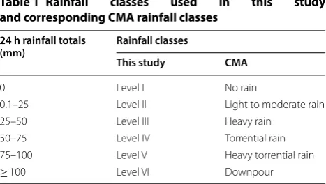
According to rainfall intensity classification from China Meteorological Administration (CMA), 24 h rainfall totals are linearly binned into six classes in this study. The six rainfall classes and their corresponding CMA rainfall classes are given in Table 1. As we introduced before, the near-surface shear wave velocity is subjected to a vari-ety of conditions (such as groundwater level, incidence angles of incoming waves, temperature, earth tide and so on). Comparing with a scatter plot of the single meas-urements of seismic velocity versus the rainfall intensity, the rainfall intensity classification is designed for pro-ducing an averaging estimation of the seismic velocity to
Table 1 Rainfall classes used in this study and corresponding CMA rainfall classes
24 h rainfall totals
(mm) Rainfall classes
This study CMA
0 Level I No rain
0.1–25 Level II Light to moderate rain
25–50 Level III Heavy rain
50–75 Level IV Torrential rain
75–100 Level V Heavy torrential rain
separate the temporal influence of rainfall from velocity changes caused by other variables.
Station and record selection
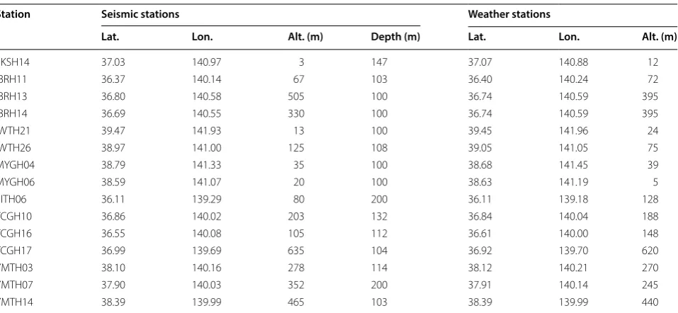
We used the earthquake and weather logging data to investigate the temporal change of near-surface shear wave velocity associated with rainfall in Japan. Fifteen seismic stations were selected for further study from 697 stations in KiK-net according to following criteria. The detailed locations of the selected seismic and weather stations are given in Table 2.
Firstly, in order to obtain enough earthquake records, Northeast Honshu (the main island of Japan) was selected as the study area because this area is prone to earthquakes. For each seismic station, we used more than 10 years of seismic records from the time when the sam-pling frequency of the seismographs is changed to 100 Hz to June 2017. The preliminary condition for a seismic sta-tion to be selected is to record at least 500 events.
Secondly, climatic character was considered in this study. In the study area, several prefectures, such as Aomori, Akita and Niigata, are located at the seaside of Sea of Japan. Due to the water vapor of the warm cur-rent in winter, it often snows heavily in these prefectures. To avoid the effect of snowfall, these prefectures were eliminated from the study area. As shown in Fig. 1, we only selected seismic stations from seven prefectures in Northeast Honshu.
Lastly, seismic stations should satisfy the requirement that the corresponding weather stations had recorded
adequate high-intensity rainfall events. For a selected seismic station, the distance between seismic station and its corresponding weather station should be less than 20 km, and the weather station should record at least two level VI events.
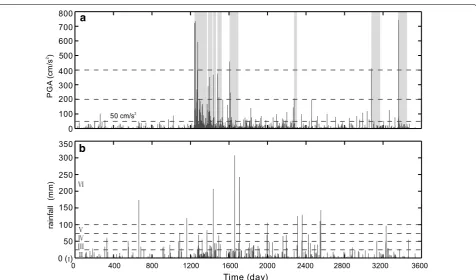
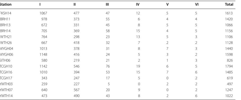
After station selection, because strong motion has an obvious impact on near-surface shear wave velocity (Takagi and Okada 2012), we then screened the seismic records for each selected station to eliminate the interfer-ences of strong motion. For selected seismic stations, the effect of strong motion can be eliminated by the following two steps. We first selected earthquake records of weak motions with peak ground acceleration (PGA) < 50 cm/ s2, and then removed records which were recorded in a period of time after strong motions with PGA > 200 cm/ s2. In this study, the influence time of strong motion depends on its PGA. Based on previous studies, for the strong motions whose PGA are between 200–400, 400– 800 and larger than 800 cm/s2, the influence times are 30, 90 and 180 days, respectively (Nakata and Snieder 2012b; Wu and Peng 2012). Figure 2 shows an example of record selection for IBRH13. The total number of seismic records for IBRH11 is reduced from 1911 to 1113 after record selection. The number of seismic records with dif-ferent rainfall classes for the selected seismic stations can be found in Table 3.
Seismic interferometry
Both cross-correlation and deconvolution can be used to retrieve the Green’s function representations
Table 2 Locations of the selected seismic stations and corresponding weather stations
Station Seismic stations Weather stations
Lat. Lon. Alt. (m) Depth (m) Lat. Lon. Alt. (m)
FKSH14 37.03 140.97 3 147 37.07 140.88 12
IBRH11 36.37 140.14 67 103 36.40 140.24 72
IBRH13 36.80 140.58 505 100 36.74 140.59 395
IBRH14 36.69 140.55 330 100 36.74 140.59 395
IWTH21 39.47 141.93 13 100 39.45 141.96 24
IWTH26 38.97 141.00 125 108 39.05 141.05 75
MYGH04 38.79 141.33 35 100 38.68 141.45 39
MYGH06 38.59 141.07 20 100 38.63 141.19 5
SITH06 36.11 139.29 80 200 36.11 139.18 128
TCGH10 36.86 140.02 203 132 36.84 140.04 188
TCGH16 36.55 140.08 105 112 36.61 140.00 148
TCGH17 36.99 139.69 635 104 36.92 139.70 620
YMTH03 38.10 140.16 278 114 38.12 140.21 270
YMTH07 37.90 140.03 352 200 37.91 140.14 245
1 2 3 4 6
5 7
129 E0 131 E0 135 E0 139 E0 142 E0 146 E0
a
31 N0
470N
3 N50
3 N90
43 N0
129 E0 131 E0
135 E0 139 E0
142 E0 146 E0 study area
1 Iwate Yamagata 2
Miyagi 3
Fukushima 4
Ibaraki 5
Tochigi 6
Saitama 7
139 5 E. 0 142 5 E. 0
35 5 N. 0
41 5. 0N
37 N0
38 5 N. 0
400N
b
139 5 E.0 142 5 E.0
140 5 E. 0 141 5 E.0
140 5 E.0 141 5 E.0
weather station seismic station
31 N0
470N
3 N50
3 N90
43 N0
35 5 N. 0
41 5.0N
37 N0
38 5 N. 0
400N
Fig. 1 a Study area. The selected seismic stations are distributed in seven prefectures of Northeast Honshu. b Magnification of the study area in Fig. 1a. The solid triangles represent the seismic stations, and the hollow circles represent the weather stations
a
b
between different receiver locations in seismic inter-ferometry. These two types of Green’s function repre-sentation have been verified as effective methods for vertical array to extract shear wave velocity in many previous studies (Miyazawa et al. 2008; Nakata and Snieder 2012a; Takagi and Okada 2012). Moreover, Takagi and Okada (2012) reported that the cross-corre-lation of the coda waves is stable in time as the decon-volution of direct waves used by Nakata and Snieder (2012a). In this study, we preferred deconvolution-based interferometry because it can eliminate the effect of the incident wavefields to get a more reasonable estimation of shear wave velocity (Nakata and Snieder 2012a). We also compared the results from coda waves and those from direct waves for three stations (i.e., IBRH11, IBRH13 and TCGH17) using deconvolution-based interferometry as shown in Additional file 2: Fig. S2. It can be found that the results from coda waves are similar to those from direct waves, because decon-volution interferometry can eliminate the effects of the incident wavefields for vertical arrays as we mentioned above.
The deconvolution function in frequency domain can be calculated by Eq. (1) and it can be converted into time domain by inverse Fourier transform.
in which s is source location, u(rb, s, ω) is the incoming wavefield recorded at the bottom sensor at location rb, (1) G(rs, s,ω)= u(rs, s,ω)
u(rb, s,ω) ≈
u(rs, s,ω)u∗(r
b, s,ω)
|u(rb, s,ω)|2+ε
u(rs, s, ω) is the corresponding wavefield recorded at the surface sensor at location rs, * is the complex conjugate and ε is a regularization parameter, set as 1% of the aver-age power spectrum of the borehole receiver (Nakata and Snieder 2012a), to enhance the stability of deconvolution function.
After computing deconvolution function, we grouped them by rainfall classes (Table 1) and then averaged them for each group. The shear wave velocities of dif-ferent rainfall classes can be extracted using cubic spline interpolation to find peak times (Fig. 3b). These times are the travel times for shear waves that propa-gate between the bottom and surface sensors. By rotat-ing the wavefields from 10° to 180° in 10° interval, we computed the shear wave velocity as a function of polarization angle. As described in Nakata and Snieder (2012a), the velocity can be separated into the isotropic and the anisotropic terms by a Fourier series expansion. The anisotropic component of the velocity is caused by shear wave splitting, which is beyond the scope of this study. The isotropic component can be calculated by averaging velocities of the eighteen directions. We assumed the splitting time to be much smaller than the travel time, and employed the isotropic component to represent the near-surface velocity.
Figure 3 shows an example of deconvolution func-tions for the EW direction in different rainfall classes at TCGH17 station. The deconvolution functions have clear peaks near the measured travel times of shear wave based on velocity profiles. The peak time of the level VI lags 4.6 ms from that of level I (Fig. 3b). It could
Table 3 Number of seismic records with different rainfall classes
Station I II III IV V VI Total
FKSH14 1067 477 47 12 5 5 1613
IBRH11 978 373 55 6 4 4 1420
IBRH13 672 331 45 8 5 5 1066
IBRH14 705 369 58 15 4 5 1156
IWTH21 764 298 23 13 5 3 1106
IWTH26 667 418 32 7 2 2 1128
MYGH04 1013 378 31 8 7 3 1440
MYGH06 1148 416 24 5 3 2 1598
SITH06 580 219 21 2 1 3 826
TCGH10 1142 546 76 19 6 5 1794
TCGH16 1010 394 53 15 7 6 1485
TCGH17 343 247 17 5 0 2 619
YMTH03 259 227 5 0 2 2 497
YMTH07 640 567 20 9 0 2 1247
be clearly observed that high-intensity rainfall has an obvious influence on near-surface shear wave velocity for TCGH17 station.
Results
We computed the shear wave velocities of different rain-fall classes from deconvolution functions and calculated the relative velocity change (dv/v) for these 15 selected stations. The relative velocity change is defined as
in which vi is the near-surface shear wave velocity for
level i.
Figure 4 depicts the relationship between the rela-tive velocity change dv/v and the rainfall classes. It can be found that the results from averaged deconvolution function are comparable with the mean values of single measurements. Meanwhile, the relative high standard deviations of single measurements indicate the neces-sity of the averaging process. As discussed in Wang et al. (2017), seismic velocity changes in Japan are subjected to nonidentical environmental factors in different areas. According to local geological, climatic and geographical conditions, we infer that the seismic velocity variations in Northeast Honshu are mainly controlled by the strong motion, precipitation and sea level changes. It also should be noted that Northeast Honshu is one of the regions with the smallest seasonal seismic velocity changes in Japan,
(2) dv/v=(vi−vI)/vI(i=II, III, IV, V, VI)
which allows detection of temporal change of seismic velocity associated with rainfall that might be masked by the strong seasonal perturbations in other areas.
It can be found that the surface shear wave velocities do not change obviously when rainfall class varies from level II to V, and the velocity decreases significantly when rainfall class reaches level VI. It can be concluded that there exists a threshold (rainfall class level VI) of the temporal influence of rainfall on near-surface shear wave velocity.
Nakata and Snieder (2012a) reported that the sta-tions located at soft rock sites are influenced more by rainfall than the stations at hard rock sites. We fol-lowed the definition of the soft and hard rock sites of their study. The estimated shear wave velocity of hard rock sites is greater than 600 m/s, while that of soft rock sites is less than 600 m/s. Among the 15 stations, there are four stations (IBRH14, MYGH04, TCGH17 and YMTH03) are located at hard rock sites. However, in this study, it did not show that stations at soft rock sites are influenced more by rainfall than stations at hard rock sites. Moreover, the relative velocity change caused by high-intensity rainfall of TCGH17 station is much higher than that of 12 stations at soft rock sites (Fig. 4). One possible interpretation is that the relative velocity change (dv/v) highly depends on the borehole depth (Takagi and Okada 2012). More detailed explana-tion can be found in “Discussion” section.
a
b
Discussion
First, we discussed the threshold of the temporal influ-ence of rainfall on the near-surface shear wave velocity. In a recent study, Dong and Lu (2016) used bender ele-ment technique to measure the dependencies of shear wave velocity on saturation for seven different types of unsaturated soils. They reported there are two thresh-olds of the influence of water content on shear wave velocity. The laboratory test results show that, as the volumetric water content varies from zero to the first threshold of around 0.15, the shear wave velocities of dif-ferent soils decrease sharply. When the water content is in the range of approximately 0.15–0.40, the shear wave velocities gradually decrease with a mild rate as the water
content increases. After the water content exceeds the second threshold of about 0.40, the shear wave velocities decrease significantly with the water content increases. The velocity reduction is mainly caused by the decreased effective stress (Dong and Lu 2016; Snieder and Beukel 2004). The detailed properties of tested soils and the clas-sifications can be found in Dong and Lu (2016).
Generally speaking, the initial water content of the in situ soil is higher than the first threshold. The water content of the surface sediment is influenced by rain-fall directly, thus the relationship between near-surface velocity and rainfall is similar to that between shear wave velocity and water content. It is not difficult to under-stand the thresholds of rainfall for different stations are Fig. 4 Relationships between the relative velocity change dv/v and the rainfall classes for 15 seismic stations from KiK‑net. The solid circular
quite similar because thresholds of water content for dif-ferent soils are about 0.4, ranging from 0.35 to 0.45.
Compared with wave velocity, wave slowness (the inverse of wave velocity) is a direct indicator of wave propagation time (the travel time is proportional to the wave slowness) mathematically, and has been widely used in geophysics and earthquake engineering (Boore and Asten 1983; Brown et al. 2002; Eisner et al. 2009; Hao and Stovas 2016; Steck 1995; Steck and Prothero 1993; Xiang et al. 1999). As shown in Fig. 5a, the threshold of the tem-poral influence of rainfall on near-surface shear wave velocity could be more clearly explained by the relation-ship between shear wave slowness and water content.
Since major velocity change is localized in shallow layer, the travel time increment is independent of the bore-hole depth. Thus we presented the relationship between travel time increment and rainfall class in Fig. 5b. Com-pared with the travel time corresponding to the rainfall class level I (no rain), the travel time increment is no more than 3×10⁻⁴ s when rainfall class varies from level II to V, and it ranges between 1×10⁻³ and 7×10⁻³ s (the mean value and standard deviation are 3.29×10⁻³ and 1.36×10⁻³ s, respectively) when the rainfall class reaches level VI.
To get a deeper insight into the temporal influence of rainfall on near-surface shear wave velocity, we proposed a one-dimensional model to estimate travel time incre-ments. As shown in Fig. 6, P, H, Δθ and ΔS are rainfall totals, permeate depth, the variation of surface volumet-ric water content and variation of shear wave slowness after rain, respectively. The travel time increment Δt can be obtained as follows:
in which v1 and v2 are surface shear wave velocities before and after rain, respectively. In the calculation model, we assumed the rainfall is completely and evenly absorbed by the surface sediments. Hence we can get:
(3)
t= H v2−
H
v1 =H·S
(4) P =H·(θ2−θ1)
a
b
Fig. 5 (a) Relationships between shear wave slowness and volumetric water content for seven different types of soil (Dong and Lu, 2016). (b) Relationship between travel time increment and rainfall class for each seismic station (the gray lines). Black line represents cross‑plot between the mean travel time increment and rainfall class with error bars. The relationship between shear wave slowness and volumetric water content has a similar pattern with that of travel time increment and rainfall class
in which θ1 and θ2 are surface volumetric water content before and after rain, respectively. Combining Eqs. (3) and (4) yields:
Equations (5) and (6) can be used to estimate the per-meate depth and the travel time increment, respec-tively. From Fig. 5a, when the rainfall class reaches level VI, the variation of volumetric water content Δθ and variation of shear wave slowness ΔS can be estimated as approximately 20–40% and 4–10×10−3 s/m, respectively. And the rainfall total of level VI is about 100–200 mm according to the meteorological records. Hence we can get H= 0.25–1.0 m and Δt= 1–10×10−3 s for level VI. The result of H is consistent with the previous analyti-cal solutions for one-dimensional, transient infiltration (Srivastava and Yeh 1991) and it reveals that the tempo-ral influence of rainfall on travel time increment is only related to surface sediments (around 1 m, which is far less than the borehole depth). The estimated travel time increments are basically consistent with our results of observation (Fig. 5b), which validate the presented for-mula of Eq. (6).
Conclusions
In this study, we investigated temporal change of near-surface shear wave velocity associated with rainfall using earthquake and weather logging data in Northeast Hon-shu. The relative velocity reduction is observed as several percent under high-intensity rainfall. The relationship between near-surface velocity and rainfall is similar to that between shear wave velocity and water content. Based on the results of observation, we proposed a one-dimensional model to explain the temporal influence of rainfall on near-surface shear wave velocity. The conclu-sions of this study are summarized as follows:
1. The near-surface shear wave velocity does not change obviously under low-intensity rainfall, while it decreases significantly when the rainfall intensity exceeds a threshold (around 100 mm of 24 h rainfall total).
2. Compared with the travel time of no rain, the travel time increment of low-intensity rainfall is no more than 3×10⁻⁴ s, while that of high-intensity
rain-3. The velocity change caused by rainfall is directly related to the dependency of velocity on saturation of surface sediments (around 1 m). According to the one-dimensional model proposed in this study, the travel time increment can be estimated by multi-plying rainfall P and the ratio of the variation of the shear wave slowness ΔS to variation of volumetric water content Δθ. This model can give a preliminary estimation of the temporal influence of rainfall on near-surface shear wave velocity.
Additional files
Additional file 1: Fig.S1. Relationships between the relative velocity change and the rainfall classes for different accumulated periods of rainfall amounts.
Additional file 2: Fig.S2. Relationships between the relative velocity change and the rainfall classes for direct waves and coda waves.
Abbreviations
CMA: China Meteorological Administration; JMA: Japan Meteorological Agency; NIED: National Research Institute for Earth Science and Disaster Resilience; PGA: Peak ground acceleration.
Authors’ contributions
YM and YS participated in acquisition of seismic and meteorologic data. YS processed the obtained data. YS and SYW drafted the manuscript. YM, YS, and SYW contributed to the planning of this study and interpretation of the data. All authors read and approved the final manuscript.
Acknowledgements
It is gratefully acknowledged that NIED and JMA provided the earthquake and weather data, respectively.
Competing interests
The authors declare that they have no competing interests.
Availability of data and materials
The earthquake and weather data were provided by National Research Institute for Earth Science and Disaster Prevention and Japan Meteorological Agency, respectively. The earthquake records are available on http://www. kyosh in.bosai .go.jp/kyosh in/quick /index _en.html. The weather records are available on http://www.data.jma.go.jp/obd/stats /etrn/index .php.
Consent for publication
Not applicable.
Ethics approval and consent to participate
Not applicable.
Funding
This study was financially supported by the National Key R&D Program of China (No. 2016YFC0800200), the National Science Foundation of China (No. 51778260), and the China Postdoctoral Science Foundation (No. 2018M642845).
Publisher’s Note
Received: 30 August 2018 Accepted: 4 December 2018
References
Ahmadi MM, Paydar NA (2014) Requirements for soil‑specific correlation between shear wave velocity and liquefaction resistance of sands. Soil Dyn Earthq Eng 57(2):152–163. https ://doi.org/10.1016/j.soild yn.2013.11.001
Aoi S, Kunugi T, Fujiwara H (2004) Strong‑motion seismograph network oper‑ ated by NIED: K‑net and KiK‑net. J Jpn Assoc Earthq Eng 4(3):65–74. https ://doi.org/10.5610/jaee.4.3_65
Bakulin A, Calvert R (2006) The virtual source method: theory and case study. Geophysics 71(4):SI139–SI150. https ://doi.org/10.1190/1.22161 90 Boore DM, Asten MW (1983) Comparisons of shear‑wave slowness in the Santa
Clara Valley, California, using blind interpretations of data from invasive and noninvasive methods. Bull Seismol Soc Am 98(4):1983–2003. https :// doi.org/10.1785/01200 70277
Borcherdt RD (1994) Estimates of site‑dependent response spectra for design (methodology and justification). Earthq Spectra 10(4):617–653. https :// doi.org/10.1193/1.15857 91
Brenguier F, Shapiro NM, Campillo M, Ferrazzini V, Duputel Z, Coutant O et al (2008) Towards forecasting volcanic eruptions using seismic noise. Transl World Seismol 1(2):126–130. https ://doi.org/10.1038/ngeo1 04 Brenguier F, Clarke D, Aoki Y, Shapiro NM, Campillo M, Ferrazzini V (2011) Moni‑
toring volcanoes using seismic noise correlations. CR Geosci 343(8):633– 638. https ://doi.org/10.1016/j.crte.2010.12.010
Brenguier F, Campillo M, Takeda T, Aoki Y, Shapiro NM, Briand X, Emoto K, Miyake H (2014) Mapping pressurized volcanic fluids from induced crustal seismic velocity drops. Science 345(6192):80–82. https ://doi. org/10.1126/scien ce.12540 73
Brown LT, Boore DM, Stokoe KH (2002) Comparison of shear‑wave slowness profiles at 10 strong‑motion sites from noninvasive SASW measurements and measurements made in boreholes. Bull Seismol Soc Am 92(8):3116– 3133. https ://doi.org/10.1785/01200 20030
Clements T, Denolle MA (2018) Tracking groundwater levels using the ambient seismic field. Geophys Res Lett 45(13):6459–6465. https ://doi. org/10.1029/2018G L0777 06
Choi Y, Stewart JP (2005) Nonlinear site amplification as function of 30 m shear wave velocity. Earthq Spectra 21(1):1–30. https ://doi.org/10.1193/1.18565 35
Dong Y, Lu N (2016) Dependencies of shear wave velocity and shear modulus of soil on saturation. J Eng Mech 142(11):4016083. https ://doi. org/10.1061/(ASCE)EM.1943‑7889.00011 47
Eisner L, Fischer T, Rutledge JT (2009) Determination of S‑wave slowness from a linear array of borehole receivers. Geophys J R Astron Soc 176(1):31–39. https ://doi.org/10.1111/j.1365‑246X.2008.03939 .x
Hao Q, Stovas A (2016) P‑wave slowness surface approximation for tilted orthorhombic media. Geophysics 81(3):C99–C112. https ://doi. org/10.1190/GEO20 15‑0440.1
Hardin BO, Black WL (1968) Closure on vibration modulus of normally consoli‑ dated clay. J Soil Mech Found Div 94(2):353–370
Hillers G, Campillo M (2016) Fault zone reverberations from cross‑correlations of earthquake waveforms and seismic noise. Geophys J Int 204(3):1503– 1517. https ://doi.org/10.1093/gji/ggv51 5
Hillers G, Campillo M, Ma KF (2014) Seismic velocity variations at TCDP are controlled by MJO driven precipitation pattern and high fluid discharge properties. Earth Planet Sci Lett 391(2):121–127. https ://doi.org/10.1016/j. epsl.2014.01.040
Hillers G, Benzion Y, Campillo M, Zigone D (2015a) Seasonal variations of seismic velocities in the San Jacinto Fault area observed with ambient seismic noise. Geophys J Int 202(2):920–932. https ://doi.org/10.1093/gji/ ggv15 1
Hillers G, Retailleau L, Campillo M, Inbal A, Ampuero JP, Nishimura T (2015b) In situ observations of velocity changes in response to tidal deformation from analysis of the high‑frequency ambient wavefield. J Geophys Res Solid Earth 120(1):210–225. https ://doi.org/10.1002/2014J B0113 18 Hobiger M, Wegler U, Shiomi K, Nakahara H (2012) Coseismic and postseis‑
mic elastic wave variations caused by the 2008 Iwate‑Miyagi Nairiku
earthquake, Japan. J Geophys Res Solid Earth 117(B9):B09313. https ://doi. org/10.1029/2012j b0094 02
Lee CJ, Hung WY, Tsai CH, Chen T, Tu Y, Huang CC (2014) Shear wave velocity measurements and soil‑pile system identifications in dynamic centrifuge tests. Bull Earthq Eng 12(2):717–734. https ://doi.org/10.1007/s1051 8‑013‑9545‑1
Mainsant G, Larose E, Brönnimann C, Jongmans D, Michoud C, Jaboyedoff M (2012) Ambient seismic noise monitoring of a clay landslide: toward failure prediction. J Geophys Res Earth Surf 117:F01030. https ://doi. org/10.1029/2011J F0021 59
Mehta K, Snieder R, Graizer V (2007) Extraction of near‑surface properties for a lossy layered medium using the propagator matrix. Geophys J Int 169(1):271–280. https ://doi.org/10.1111/j.1365‑246X.2006.03303 .x Meier U, Shapiro NM, Brenguier F (2010) Detecting seasonal variations in
seismic velocities within Los Angeles basin from correlations of ambient seismic noise. Geophys J Int 181(2):985–996. https ://doi.org/10.1111/ j.1365‑246x.2010.04550 .x
Miyazawa M, Snieder R, Venkataraman A (2008) Application of seismic interfer‑ ometry to extract P‑ and S‑wave propagation and observation of shear‑ wave splitting from noise data at Cold Lake, Alberta, Canada. Geophysics 73(4):D35–D40. https ://doi.org/10.1190/1.29371 72
Nakata N, Snieder R (2011) Near‑surface weakening in Japan after the 2011 Tohoku‑Oki earthquake. Geophys Res Lett 38(17):L17302. https ://doi. org/10.1029/2011G L0488 00
Nakata N, Snieder R (2012a) Estimating near‑surface shear wave velocities in Japan by applying seismic interferometry to KiK‑net data. J Geophys Res Solid Earth 117(B1):B01308. https ://doi.org/10.1029/2011J B0085 95 Nakata N, Snieder R (2012b) Time‑lapse change in anisotropy in Japan’s
near surface after the 2011 Tohoku‑Oki earthquake. Geophys Res Lett 39(11):L11313. https ://doi.org/10.1029/2012G L0519 79
Niu F, Silver PG, Daley TM, Cheng X, Majer EL (2008) Preseismic velocity changes observed from active source monitoring at the Parkfield SAFOD drill site. Nature 454(7201):204–208. https ://doi.org/10.1038/natur e0711 1 Obermann A, Planès T, Larose E, Campillo M (2013) Imaging preeruptive and
coeruptive structural and mechanical changes of a volcano with ambient seismic noise. J Geophys Res Solid Earth 118(12):6285–6294. https ://doi. org/10.1002/2013J B0103 99
Ohmi S, Hirahara K, Wada H, Ito K (2008) Temporal variations of crustal structure in the source region of the 2007 Noto Hanto Earthquake, central Japan, with passive image interferometry. Earth Planets Space 60(10):1069–1074. https ://doi.org/10.1186/BF033 52871
Okada Y, Kasahara K, Hori S, Obara K, Sekiguchi S, Fujiwara H et al (2004) Recent progress of seismic observation networks in Japan‑Hi‑net, F‑net, K‑net and KiK‑net. Earth Planets Space 56(8):xv–xxviii. https ://doi. org/10.1186/BF033 53076
Pilz M, Parolai S, Bindi D, Saponaro A, Abdybachaev U (2014) Combining seis‑ mic noise techniques for landslide characterization. Pure Appl Geophys 171(8):1729–1745. https ://doi.org/10.1007/s0002 4‑013‑0733‑3 Richter T, Sen‑Schönfelder C, Kind R, Asch G (2014) Comprehensive observa‑
tion and modeling of earthquake and temperature‑related seismic velocity changes in Northern Chile with passive image interferometry. J Geophys Res Solid Earth 119(6):4747–4765. https ://doi.org/10.1002/2013J B0106 95
Rivet D, Brenguier F, Cappa F (2015) Improved detection of preeruptive seismic velocity drops at the Piton de La Fournaise volcano. Geophys Res Lett 42(15):6332–6339. https ://doi.org/10.1002/2015G L0648 35
Sen‑Schönfelder C, Wegler U (2006) Passive image interferometry and seasonal variations of seismic velocities at Merapi volcano, Indonesia. Geophys Res Lett 33(21):L21302. https ://doi.org/10.1029/2006G L0277 97 Snieder R, Beukel AVD (2004) The liquefaction cycle and the role of drainage
in liquefaction. Granul Matter 6(1):1–9. https ://doi.org/10.1007/s1003 5‑003‑0151‑9
Srivastava R, Yeh TCJ (1991) Analytical solutions for one‑dimensional, transient infiltration toward the water table in homogeneous and layered soils. Water Resour Res 27(5):753–762
Steck LK (1995) Simulated annealing inversion of teleseismic P‑wave slowness and azimuth for crustal velocity structure at Long Valley Caldera. Geophys Res Lett 22(4):497–500. https ://doi.org/10.1029/94GL0 3050
Takagi R, Okada T (2012) Temporal change in shear velocity and polarization anisotropy related to the 2011 M9.0 Tohoku‑Oki earthquake exam‑ ined using KiK‑net vertical array data. Geophysical Research Letters 39(9):L09310. https ://doi.org/10.1029/2012G L0513 42
Toksoz MN, Cheng CH, Timur A (1976) Velocities of seismic waves in porous rocks. Geophysics 41(4):621–645. https ://doi.org/10.1190/1.14406 39 Tsai VC (2011) A model for seasonal changes in GPS positions and seismic
wave speeds due to thermoelastic and hydrologic variations. J Geophys Res Solid Earth 116(B4):B04404. https ://doi.org/10.1029/2010J B0081 56 Voisin C, Guzmán MAR, Réfloch A, Taruselli M, Garambois S (2017) Groundwa‑
ter monitoring with passive seismic interferometry. J Water Resour Prot 09(12):1414–1427. https ://doi.org/10.4236/jwarp .2017.91209 1 Wang Q‑Y, Brenguier F, Campillo M, Lecointre A, Takeda T, Aoki Y (2017) Sea‑
sonal crustal seismic velocity changes throughout Japan. J Geophys Res Solid Earth 122(10):7987–8002. https ://doi.org/10.1002/2017J B0143 07 Wegler U, Sens‑Schönfelder C (2010) Fault zone monitoring with passive
image interferometry. Geophys J R Astron Soc 168(3):1029–1033. https :// doi.org/10.1111/j.1365‑246X.2006.03284 .x
Wegler U, Lühr BG, Snieder R, Ratdomopurbo A (2006) Increase of shear wave velocity before the 1998 eruption of Merapi volcano (Indonesia). Geo‑ phys Res Lett 33(9):L09303. https ://doi.org/10.1029/2006G L0259 28 Wu C, Peng Z (2012) Long‑term change of site response after the Mw, 9.0
Tohoku earthquake in Japan. Earth Planets Space 64(12):1259–1266. https ://doi.org/10.5047/eps.2012.05.012
Xiang D, Hsu NN, Blessing GV (1999) Imaging of acoustic surface wave slow‑ ness. Appl Phys Lett 74(15):2236–2238. https ://doi.org/10.1063/1.12381 2 Xu X, Su L, Zhang G, Zhu H (2017) Analysis on shear wave velocity structure of
a gravel landslide based on dual‑source surface wave method. Landslides 14(3):1127–1137. https ://doi.org/10.1007/s1034 6‑016‑0780‑9