Bayesian Methods for Exploratory Functional Data Analysis and Existence Theorems for Solutions to Nonlinear Differential and Difference Equations.

SUAREZ, ADAM JUSTIN. Bayesian Methods for Exploratory Functional Data Analysis and Existence Theorems for Solutions to Nonlinear Differential and Difference Equations. (Under the direction of Dr. Subhashis Ghosal and Dr. Jesús Rodríguez.)

This document is comprised of two parts: two chapters on the subject of Bayesian functional data analysis, and two chapters on the solvability of nonlinear equations.

Chapter 2 deals with the clustering of functional data. The use of exploratory methods is an important step in the understanding of data. When clustering functional data, most methods use traditional clustering techniques on a vector of estimated basis coefficients, assuming that the underlying signal functions live in the L2-space. Bayesian methods use models which imply the belief that some observations are realizations from some signal plus noise models with identical underlying signal functions. The method we propose differs in this respect: we employ a model that does not assume that any of the signal functions are truly identical, but possibly share many of their local features, represented by coefficients in a multiresolution wavelet basis expansion. We cluster each wavelet coefficient of the signal functions using conditionally independent Dirichlet process priors, thus focusing on exact matching of local features. We then demonstrate the method using two datasets from different fields to show broad application potential.

Chapter 3 studies the area of principal components analysis (PCA), which has seen relatively few contributions from the Bayesian school of inference. In this chapter, we propose a Bayesian method for PCA in the case of functional data observed with error. We suggest modeling the covariance function by use of an approximate spectral decomposition, leading to easily interpretable parameters. We perform model selection, both over the number of principal components and the number of basis functions used in the approximation. We study in depth the choice of using the implied distributions arising from the inverse Wishart prior and prove a convergence theorem for the case of an exact finite dimensional representation. We also discuss computational issues, as well as the care needed in choosing hyperparameters. A simulation study is used to demonstrate competitive performance against a recent frequentist procedure, particularly in terms of the principal component estimation. Finally, we apply the method to a real dataset, where we also incorporate model selection on the dimension of the finite basis used for modeling.

by

Adam Justin Suarez

A dissertation submitted to the Graduate Faculty of North Carolina State University

in partial fulfillment of the requirements for the Degree of

Doctor of Philosophy

Statistics and Mathematics

Raleigh, North Carolina 2016

APPROVED BY:

Dr. Subhashis Ghosal

Co-chair of Advisory Committee Co-chair of Advisory CommitteeDr. Jesús Rodríguez

Dr. Stephen Schecter Dr. Eric Stone

Thank you to my advisors for all of their support and encouragement. It has been a great honor to work so closely with both of them. Thank you also to my entire committee, each one of whom has had a major influence on my graduate career.

Thank you to Sarah Thomson, who not only supported me through my decision to apply to graduate school, but has been one of the major inspirations in my life, more than she could ever know. Thank you to all of the great friends that have supported me during my time in Raleigh, specifically David and Laura Vock, Sarah Hale, and Christopher Krut. Thank you to my amazing girlfriend, Jessalyn Crawford, whose love and support has made the most stressful time of my life also the most enjoyable. Thank you again to my parents to whom I owe everything.

LIST OF TABLES. . . vii

LIST OF FIGURES . . . viii

Chapter 1 Bayesian Methods for Exploratory Functional Data Analysis . . . 1

Chapter 2 Bayesian Clustering of Functional Data Using Local Features. . . 3

2.1 Introduction . . . 3

2.2 The Model . . . 5

2.3 Prior Distributions . . . 7

2.4 The Similarity Matrix and Clustering . . . 9

2.5 Interpretation of Prior Characteristics . . . 10

2.6 Convergence Results . . . 11

2.7 Computation . . . 13

2.8 Applications to Data . . . 14

2.8.1 EEG Data . . . 15

2.8.2 Canadian Weather Data . . . 16

2.9 Discussion . . . 17

2.10 Proofs . . . 30

Chapter 3 Bayesian Estimation of Principal Components for Functional Data . . . 37

3.1 Introduction . . . 37

3.2 Background . . . 38

3.3 Model, Prior Specification, and Posterior Computation . . . 40

3.3.1 Model and Priors . . . 41

3.3.2 Low Rank Model . . . 42

3.3.3 Model Choice . . . 43

3.3.4 Choice of Hyperparameters . . . 43

3.3.5 Posterior Computation . . . 44

3.3.6 Alternative Posterior Computation . . . 45

3.4 Asymptotic Results . . . 47

3.5 Simulation Study . . . 48

3.5.1 Description of FACE . . . 48

3.5.2 Results . . . 49

3.6 Canadian Weather Data . . . 51

3.7 Discussion . . . 54

3.8 Proofs . . . 60

5.1 Introduction . . . 66

5.2 Generalities . . . 67

5.3 Differential Equations . . . 69

5.4 Difference Equations . . . 79

Chapter 6 Existence of Solutions to Nonlinear Boundary Value Problems. . . 85

6.1 Introduction . . . 85

6.2 General Strategy . . . 86

6.3 Preliminaries . . . 89

6.4 Nonlinear Systems . . . 89

6.5 Comparison to Previous Results . . . 93

6.6 Example . . . 95

6.7 Discussion . . . 96

Figure 2.1 EEG Data: Plot of the proportion of pairs of data points with distance less than a given value. . . 20 Figure 2.2 EEG Data - Top: Dendrogram generated using the dissimilarity matrix by

Ward’s method. The stars on the margins represent observations from the fifth group (suspected seizure activity). Bottom: Groups formed when the dendrogram is cut to yield 2 groups. Dashed lines are pointwise posterior means for the observations, and solid blues lines are the pointwise group average. These figures correspond to M =20. . . 21

Figure 2.3 EEG Data: Adjusted Rand index comparison between 3 hyperparameter choices and a default method. The clustering was evaluated compared to the “true” clustering defined by whether the observation was from known seizure

activity. . . 22 Figure 2.4 EEG Data: Clustering the EEG data by cutting the tree at 12 groups. This

corresponds to the last cut point that still maintains a relatively high adjusted Rand index. . . 23 Figure 2.5 Weather Data -Top: Dendrogram created from the dissimilarity matrix by

Ward’s method. Bottom: Map of the cities coded by symbol in color to represent the groups formed when the dendrogram is cut to yield 6 groups. These plots correspond toM =10. . . 24

Figure 2.6 Weather Data - Dendrogram and heatmap created from the dissimilarity matrix by Ward’s method. This plot corresponds to M =10. . . 25

Figure 2.7 Weather Data: Boxplots of the number of distinct points in a given MCMC step for a range of coefficients and for different values of the mass parameter, M. The coefficient numbers were chosen arbitrarily to show the clustering at different resolution levels. . . 26 Figure 2.8 Weather Data: Clustering formed by cutting at 6 groups for M =1. For

each group, the observed functional data are plotted on the same axes. . . 27 Figure 2.9 Weather Data: Clustering formed by cutting at 6 groups for M =10. For

each group, the observed functional data are plotted on the same axes. . . 28 Figure 2.10 Weather Data: Clustering formed by cutting at 6 groups for M =20. For

each group, the observed functional data are plotted on the same axes. . . 29 Figure 3.1 Simulation Study: Boxplots for the simulation results corresponding toκ1

with the left box (red color) representing the proposed Bayesian procedure, and the right (black) representing the FACE procedure. The value above each pair represents the proportion of data sets in which the Bayesian procedure performed superiorly. . . 51 Figure 3.3 Simulation Study: Boxplots for the simulation results corresponding toκ2

used for both the truth and the prior. Results are shown in pairs, with the left box (red color) representing the proposed Bayesian procedure, and the right (black) representing the FACE procedure. The value above each pair represents the proportion of data sets in which the Bayesian procedure performed superiorly. . . 52 Figure 3.4 Simulation Study: Boxplots for the simulation results corresponding toκ2

used for the truth and κ1 used for the prior. Results are shown in pairs, with the left box (red color) representing the proposed Bayesian procedure, and the right (black) representing the FACE procedure. The value above each pair represents the proportion of data sets in which the Bayesian procedure performed superiorly. . . 53 Figure 3.5 Simulation Study: Examples of the posterior distribution of models for each

of the four experimental conditions. Row 1 corresponds to κ1 as the prior, and column 1 corresponds to κ1 as the truth. The other row and column correspond to κ2. . . 55 Figure 3.6 Canadian Weather Data: Posterior probabilities for each model,(J,K). Only

models 1_≤K ≤J ≤25had prior mass. . . 56

Figure 3.7 Canadian Weather Data: Observations (dots) along with pointwise posterior means (lines). The posterior means are the mean of HJUKβi,K over(J,K). 56

Figure 3.8 Canadian Weather Data: Full posterior mean of the covariance function over all (J,K) pairs. . . 57 Figure 3.9 Canadian Weather Data: First four FPCAs corresponding to the full posterior

Chapter

1

Bayesian Methods for Exploratory Functional

Data Analysis

Exploratory methods in statistics become increasingly necessary when the dimensionality of the data increases. Because of this, they are a primary focus of multivariate data analysis. With the growing popularity of functional data, many of the methods from multivariate statistics have been adapted for the special structures that functional data present. When applying Bayesian methods to functional data, these particular features lead to important considerations in the specification of prior distributions.

Particular to functional data, there are typically two classes of models: models for perfectly observed functional data, and models for noisy functional data. In this document, we only consider models for functional data observed with error (noisy data). Related to this, the main result of Chapter 2 is an asymptotic result in terms of this error variance converging to0.

In the next two chapters we consider two Bayesian methods for exploring functional data: hierarchical clustering and principal components analysis. Both of these methods seek to discover structure within the data.

then use a deterministic hierarchical clustering technique with this matrix as its input. Particular to functional data, we model using a wavelet decomposition of the individual functions. This directly influences the prior choice since wavelet decompositions are known to be sparse in many situations. The intricacies of this model are discussed in detail in the next chapter.

Chapter

2

Bayesian Clustering of Functional Data Using

Local Features

2.1

Introduction

Exploratory analysis of new data is an important first step to understanding many scientific questions. Cluster analysis is a popular tool in exploratory analysis to try to discover underlying group structure present in the data. The idea behind cluster analysis is to define sets of data points which are similar within groups and dissimilar between groups. The main question that is raised is what concept to use to define “similar”. Many clustering techniques (especially hierarchical clustering) can be implemented based solely on a matrix of pairwise similarities (equivalently, dissimilarities). One obvious choice for a notion of similarity is that of distance, which is nearly always available since data are most commonly assumed to be elements of some metric space. However, distances are not the only possible choices, and their usage may miss some important qualitative features. A similarity index can be chosen to be any function of two arguments, as long as it represents our qualitative view of what makes two observations similar.

functional data. Tarpey & Kinateder [3] generalized the k-means clustering to the functional data setting, and proved results analogous to those of multivariate k-means. James & Sugar [4] used a random effects model to cluster sparsely sampled functional data, and dealt with the situation where the data are not observed on the same fixed time grid. One extension we do not pursue is heteroscedasticity, which was studied in Serban [5]. Functional data can often lead to viewing multiple time series in a new light. For a review of clustering of time series see Liao [6].

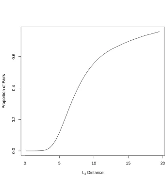
We shall not choose to define similarity in terms of distance; instead, we define a similarity function, for functions with a finite wavelet basis expansion, that strongly encourages exact matches of coefficients, meaning that the corresponding observations come from the same component of the population. Since the observed functional data include error, we use a model-based approach to estimate the true functions and use the posterior distribution of the basis coefficients to compute an estimated true similarity index. In a Bayesian setting, Ray & Mallick [7] used a truncated wavelet basis expansion and a Dirichlet process prior on their unknown joint distribution. Crandell & Dunson [8] extended this model to species sampling model priors, and also allowed the basis to be unknown. Both of these approaches cluster curves based on all of their basis coefficients jointly. By a well-known clustering property of the Dirichlet process, this implies the prior belief that some of the underlying functions have all wavelet coefficients identical, and hence, the functions themselves are identical. Often, this would not be an acceptable assumption, and this is one aspect in which the current chapter differs from most previous work. Petrone et al. [9] also dealt with this problem using “canonical curves,” from which pieces of the observed functions are drawn. For example, Figure 2.1 shows, for the EEG data discussed later, how very few pairs of data points are within a distance that would be a reasonable estimate of the error standard deviation. If the procedure of Ray & Mallick [7] were used on this data, very few observations would have positive posterior probability of sharing underlying functions (see Section 2.8).

We assign priors on the wavelet coefficients independently, where each individual coefficient gets a Dirichlet process prior distribution. The Dirichlet process allows for exact coefficient matches between functions while allowing for new values to arise also. The strength of the model is in the Bayesian approach, where the underlying coefficients across subjects are seen as exchangeable but correlated, and hence, allow for shared learning among them.

present theoretical results relating to the interpretation of the center measure of our prior, and, additionally, provide asymptotic justification of the clustering performance of our method by analyzing the small variance performance. We then demonstrate the method’s use on real datasets, and show competitive performance on a dataset with a known true clustering.

2.2

The Model

There are two common models, closely related in the asymptotic sense, that can be used to describe functional data. First let {φk:k∈Z} ∪ {ψj k: j ∈N,k ∈Z} be a given wavelet basis in

the multiresolution framework. In particular, we consider the space L2[0, 1] and the family called

wavelets on the interval [10]. The first model can be viewed as a problem of measurement error, where there is a true function, fi ∈L2([0, 1]), but when we measure it at a point tj ∈[0, 1], we

only see a noisy version, so that

Yi(tj) =fi(tj) +εi j, (2.1)

where εi j is normally distributed with mean 0 and varianceσ2, and independent across i and j.

We shall assume that all functions are observed on the same fixed time grid, and that the total number of time points is a power of 2,n =2m; this is done mainly for computational convenience

since we will employ the discrete wavelet transform (DWT). Let Yi= (Yi(t1), . . . ,Yi(tn))t, fi =

(fi(t1), . . . ,fi(tn))t, and εi = (εi1, . . . ,εi n)t. If we let W denote the n ×n orthogonal matrix

corresponding to the DWT for a certain wavelet family, then our model can be transformed to

W Yi=W fi+Wεi. (2.2)

One important property of the multivariate normal distribution is its rotational invariance, which implies that Wεi=d εi, meaning equal in distribution. Throughout, we shall use φ_σ to represent

the Lebesgue density of the normal distribution with mean zero and varianceσ2_. The second model is the so-called Gaussian white noise model, given by

where Bi(·) are independent Wiener processes (Brownian motions) on [0, 1]. This corresponds to

ideal observations of continuously sampled functions. Now let

a_k(i)=

Z 1

0

φk(t)d Yi(t), α(

i)

k =

Z 1

0

φk(t)fi(t)d t,

b_{j k}(i)=

Z 1

0

ψj k(t)d Yi(t), β(

i)

j k =

Z 1

0

ψj k(t)fi(t)d t,

¯

e_k(i)=σ

Z 1

0

φk(t)d Bi(t), e(

i)

j k =σ

Z 1

0

ψj k(t)d Bi(t).

Due to the properties of stochastic integrals with respect to the Wiener process, all of the e¯_k(i) and

e_{j k}(i) are independent and normally distributed with mean 0 and varianceσ2. The model implied

on the wavelet coefficients by (2.3) is then

a_k(i)=α_k(i)+e¯_k(i), b_{j k}(i)=β_{j k}(i)+e_{j k}(i). (2.4)

For the finite (measurement error) model, our decomposition is for k =0, . . . , 2j ₋1, and

j =0, . . . ,m−1. Note thatm is not a parameter, but the assumed length (in terms of its base 2 logarithm) of each observation vector. In the infinite (random function) model, j can range over the natural numbers. In both models, we only need k =0 for the scaling coefficient, α(₀i). Our

procedure focuses mainly on the detail coefficients, {β(j ki)}, so we shall rarely mention the scaling

coefficient. On the detail coefficients, for both models, the observed coefficients can be represented as

b_{j k}(i)ind∼ N(β_{j k}(i),σ2). (2.5)

2.3

Prior Distributions

One of the attractive aspects of using a wavelet expansion for modeling is that, for many functions, the coefficients are sparse. This knowledge is easily incorporated in the prior distributions placed on the wavelet coefficients. If the error is normally distributed, a conjugate prior on the coefficients is given by independent normal priors. Since we know that some of the coefficients are identically zero, we can incorporate a point mass at 0into the prior. Specifically, the prior, for i =1, . . . ,N,

β(i)

j k

ind

∼ πjN(0,τ2_j) + (1−πj)δ0, (2.6a)

σ2

∼IG(a,b), (2.6b)

where δ0 is a point mass at 0 and IG stands for inverse gamma. The first coefficient, α0, is known as the scaling coefficient, and is usually modeled differently, with a vague prior. In our case, we simply assume that the observations have been detrended, so that the value of α0 is identically 0. Abramovich et al. [11] showed that under certain conditions on the mother wavelet, choices of the hyperparameters in this model will guarantee that the corresponding random functions almost surely lie in specific Besov spaces (denoted by Bs

p,q). In particular,

τ2

j =ν1σ22−γ1j, πj =min(1,ν22−γ2j), (2.7) for j =0, 1, . . . , and constants ν₁,ν₂,γ₁,γ₂, provide the desired interpretation. To be specific, if γ2≥1 andγ1≥0, then the random function drawn from this prior, fi, is almost surely an element

of Bs

p,q if and only if

s+1

2− γ2

p −

γ1

2 <0, if q<∞, (2.8a)

s+1

2− γ2

p −

γ1

2 =0, if q=∞. (2.8b)

vectorsβi={β

(i)

j k}j,k in the following manner: β1, . . . ,βN

i i d

∼ F, F ∼DP(M,G0), (2.9)

where G0 was the product of the priors from Abramovich et al. [11] over j and k, and DP(M,G0) stands for the Dirichlet process with center measure G0 and concentration M. This induces a posterior distribution over partitions of the data, but also implies the prior belief that some true functions are identically equal. When this is not a reasonable assumption, other choices should be made.

Our strategy for placing priors on the true wavelet coefficients is to do so independently for each coefficient using Dirichlet process priors, with center measures corresponding to the usual parametric models often used for modeling by wavelets. Thus, instead of modeling all the coefficients jointly, as in Ray & Mallick [7], they will be done so independently. We also considerσ2 to be unknown, and for this reason, we scale the variance in the base measure in the traditional manner. The full model is therefore, ∀ j,k,

b_{j k}(i)|βj k(i),σ

ind

∼ N(β_{j k}(i),σ2), (2.10a) β(1)

j k, . . . ,β

(N)

j k |Gj k iid∼Gj k, (2.10b)

Gj k∼DP(M,G_{j k}0 ), (2.10c)

G_{j k}0 =πjN(0,σ2τ2j) + (1−πj)δ0 (2.10d)

σ2

∼IG(a,b). (2.10e)

Across levels of(j,k), the random variables, {Gj k}, are independent. If X1,X2, . . .|F iid

∼F where F ∼DP(M,G0), then the predictive distribution of the sequence satisfies:

P(Xn+1∈ ·|X1, . . . ,Xn) =

M

M+nG0+

k(n)

X

j=1

mj,n

M +nδX∗j, (2.11)

where X∗

1, . . . ,Xk∗(n) are thek(n) distinct points in the first n observations, and mj,n=#{i :Xi=

X∗

j}, for j=1, . . . ,k(n). This is the so-called Pólya urn representation of the Dirichlet process [12].

some smaller “abnormal” groups.

This model tries to capture our belief that the functional data share local features that are expressed in their wavelet expansions. We also want to incorporate the knowledge of the possibility of an exactly zero wavelet coefficient, and we do that within the base measure of the Dirichlet process prior.

Remark 2.3.1. In Section 2.5 we show that all but finitely many coefficients are zero from any realization of the prior. This motivates a different approach to constructing a prior. For all {j,k}

such that j > J_∗, let (β(_{j k}1), . . . ,β(_{j k}N)) =0. We then allow J_∗ to be random and have a Poisson distribution with parameter λ. The decay of πj and τj are now not essential, since the resulting

wavelet series is always convergent. As before, we have that the number of coefficients and levels are almost surely finite. This allows more freedom in the choice ofπj since the quick decay is no

longer needed to give us this property. It is still useful, though, to keep the point mass at zero to account for reasonable prior beliefs about the wavelet expansion. This prior seems to be a much more natural choice, and even yields the later results more easily, but comes at the price of increased computational complexity.

2.4

The Similarity Matrix and Clustering

With the goal of comparing the similarity between functions, we have many choices. Recalling that there are n=2m sampled time points, and excluding one corresponding to the scaling coefficient,

we choose to quantify the similarity between two functions using the similarity index

S(i,i0) = (2m₋1)−1

m−1

X

j=0

2j₋₁

X

k=0

1(β(j ki)=β

(i0₎

j k), (2.12)

the average number of shared wavelet coefficients. This quantity is meaningful in our model since the Dirichlet process will give positive probability to this value being nonzero. The matrix is easily estimated using posterior samples from MCMC output.

we shall employ the posterior mean matrix to provide a single output from the chosen clustering algorithm.

2.5

Interpretation of Prior Characteristics

In this section we explore and review some of the properties of the previous model of Abramovich et al. [11] for a single function (the nonparametric regression setting). Instead of studying the model under a fixed value for the hyperparameter, πj, we consider the limiting case where γ2→1 from above, whereπj is also scaled by a factor. In the following, we let γ2=1+δ and considerδ→0, so we have

πj =ν2δ2−(1+δ)j, where δ >0, δ→0. (2.13)

The reason behind this choice is to approximate the situation where γ2 =1 in the original hyperparameter choice, while keeping almost surely finiteness of the number of terms in the wavelet expansion. It is needed that ν2 be scaled by δ so that, in the limit, the quantities of interest remain finite, else they would diverge without it to balance the growth.

The following proposition would be useful for prior elicitation in the case where the approach mentioned in Remark 2.3.1 was taken. It motivates and justifies the use of a Poisson prior on the number of nonzero coefficients and resolution levels, and provides an interpretation of their hyperparameters in this setting. For a proof, see Appendix 2.10.

Proposition 2.5.1. For the infinite product of the priors specified as above, the following hold: 1. The number of nonzero wavelet coefficients is a.s. finite, and this number converges in

distri-bution to a Poisson random variable with meanν2/log(2)asδ→0.

2. The number of resolution levels with at least one nonzero coefficient is a.s. finite, and this number converges in distribution asδ_→0to a Poisson random variable with mean

lim

δ→0

∞

X

j=0

¦

2.6

Convergence Results

In the present situation, we first want to study what happens to our similarity matrix as the noise variance, σ2_{→0. This would be the situation where the noisy functional observations} are approaching the true underlying functions, respectively. For the purposes of this section, we assume the continuous model of (2.3), with the full specification in terms of the coefficients being given in (2.10a).

The asymptotic regime σ2_→0 can be understood as equivalent with averaging over _{r i.i.d.} replications of the observed scheme (2.10a)–(2.10d) with r → ∞, thus replacing σ2 by _σ2

r=σ

2_/r, with σ2 known. Since _σ2 itself controls the asymptotics in the following, it is essential to treat

σ2 _{as given, or equivalently, σ}2 _{as known and r → ∞. Although this setting contrasts with} the methodology described, this has little effect when only learning about f is the goal. More

generally, it is easy to see that the arguments given below go through ifσ2 _{is unknown, but has} a fixed upper bound. An upper-truncated inverse-gamma prior can still retain the computational conjugacy. If it is desirable to work in full generality without an upper bound for σ2, we must fully observe all replications since the sample means are sufficient only when σ2 is known. Below we forgo the full setting and treat σ2 as known so that it is sufficient to observe the sample mean of b_{j k}(i) over r replications and let r → ∞.

We assume that α(i)

0 =0 for alli =1, . . . ,N, and let

kfk2=

N

X

i=1

kfik22=

N

X

i=1

∞

X

j=0

2j₋₁

X

k=0

|βj k(i)|

2_,

where f = (f1, . . . ,fN). We also consider the Sobolev norm on the product space, defined by

kfk2_Hs

N =

N

X

i=1

∞

X

j=0

22j s_kβ(_ji_·)_k2₂.

We shall refer to this space as the N-Sobolev space, Hs

N. Note that since N is fixed, we could

have chosen to combine the N Sobolev norms using any norm for RN. The parameter, _s, relates

to the number of weak derivatives possessed by the functions which themselves live in L2([0, 1]).

We use Dr to be the set of all observations.

our interest is dependent on how we believe the data to be partitioned. We will thus be interested in knowing how our beliefs about the partition structure of the data change as r → ∞. Let P be the set of all partitions of {1, . . . ,N}, and let a typical element be denoted byp=_{A0, . . . ,AM}.

For a given j,k, let Pj k={A j k

0 ,A

j k

1 , . . . ,A

j k

Mj k} be a random partition of {1, . . . ,N}, which is a

function ofβj k defined in the following way:

β(a)

j k =0 ⇐⇒ a ∈A

j k

0 , and (2.14)

β(a)

j k =β

(b)

j k 6=0 ⇐⇒ a,b ∈A

j k

i for some i ∈ {1, . . . ,Mj k}. (2.15)

By our prior specification, it is clear that any partition structure has positive probabilitya priori. Let p₀ represent the “true” partition generated by the true values of the parameters. By a compatible model, we mean a collection of all parameter values corresponding to a single partition which is finer than p₀. By an incompatible model, we mean any collection that is not acompatible model. The following result on consistency of the posterior will be useful for studying the asymptotic properties of clustering. The techniques used in the proofs are both similar to, and certainly inspired by Lian [13]. For proofs of the following, see Appendix 2.10.

Theorem 2.6.1. Letγ1>2s+1, and assume that the true underlying functions satisfy f0∈ HNs.

Then the posterior is norm-consistent, i.e., for anyε >0, Π(kf −f₀k< ε|Dr) p

→1asr → ∞.

Lemma 2.6.1. Assume that the true vector of functions lies in _Hs

N, γ1>2s+1, and let pj k,0 be the true partition of the data for a given coefficient indexed by j,k. Then

Π(Pj k =p_{j k,0|}Dr) p

→1as r→ ∞. (2.16)

Finally we consider neighborhoods of the true full model, that is p₀=_{p_{j k,0}j k}, in the product topology. Each p_{j k,0} lives in the space, P, of all possible partitions of _{1, . . . ,N}, which is finite

and endowed with the discrete topology. Note that the entire model space is uncountable. When considering the product space, a basic neighborhood in the product topology consists of the product of finitely many singleton sets in P with infinitely many copies of P. Because of this, we easily obtain the following theorem.

Proof. First notice that N(p0) consists of the product of finitely many single point sets with an infinite number of copies of the whole space. Thus, the probability of this neighborhood is the finite product of the probabilities of each point set, each of which tends to 1by Lemma 2.6.1. Thus,

the result is proved.

2.7

Computation

Computation is done using the urn representation of the Dirichlet process prior, and we follow the procedure of Navarrete et al. [14]. The main problem in posterior computation will be the fact that we employ an atomic base measure, and this means that in the urn representation, a value can be 0, either because it is tied to a previous value, or because it was drawn

from the base measure. To simplify notation, we focus on updating one particular wavelet coefficient across observations, so we fix j,k and let βi, for i =1, . . . ,N, be the parameter for

observation i. Due to exchangeability in the Dirichlet process model, it suffices to describe the conditional posterior draws from βN| {βi}Ni=−11,{bi}

N

i=1,σ

2

and σ2_{| {β}

i}Ni=1,{bi}

N

i=1

. Similar to Section 2.2, let β∗

1, . . . ,βk∗(N−1) be the k(N −1) unique values among the first N−1 parameters.

Let mN−1={m1,N−1, . . . ,mk(N−1),N−1}, wheremj,N−1=#{1≤i ≤N :βi=β∗j}. When needed, we

shall additionally subscript quantities to designate the (j,k) level. The Gibbs sampling algorithm executes the following steps:

• Set βN equal to β_l∗ with probability proportional to

ml,N−1

M+N −1φσ(bi−β ∗

l) =

ml,N−1

M+N −1(2πσ

2₎−1/2_e{−_2σ12(bN−βl∗)2}.

• With probability proportional to

M M+N−1

Z

φσ(bN−β)d G0(β) =

M

M+N−1(2πσ

2₎−1/2

e−1/(2σ2)

×



1−πj+πj

τ2

1+τ2_j

1/2

e

b_N2τ2

j

2σ2₍1+τ2

j)



sample βN from the following distribution

π∗_δ

0+ (1−π∗)N

‚

bNτ2_j

1+τ2

j

, σ

2_τ2

j

1+τ2

j

Œ

,

where

π∗_{= 1+} πj

1₋πj

1 1+τ2

j

1/2

e

_τ2

jbN2

σ2₍1+τ2

j)

_!−1

.

• Sample σ2 _{from the following distribution:}

I G a+N n/2+X

j,k

ki j(N)/2,b+

1 2

X

i,j,k

(b_{j k}(i)−βj k(i))

2₊X

j

1 2τ2

j

X

k

kj k(N)

X

i=1

β∗

j k,i

2

!

.

• Finally, update any hyperparameters that have been added to the prior specification. The main issue to notice is that both possibilities forβN can lead to a value of 0(either being

tied to an existing point which happens to be 0, or drawing a 0 from the base measure), and this

needs to be taken into account when fitting the model, which simply requires careful bookkeeping. After each draw from these full conditionals, we need to update the unique points, along with k(N −1), and mN−1.

2.8

Applications to Data

In this section we present the usefulness of the above method by analyzing two different data sets. When presenting results, often it is convenient to display the similarity matrix after it has been used in a deterministic hierarchical clustering scheme. In particular, we apply Ward’s method of clustering [15] to the dissimilarity matrix defined by{1/S∗_(i,i0_)}N

i,i0₌₁. This method is an agglomerative method, in which a single element is joined with an existing group, so that the sum of the variances of all groups is minimized. Other hierarchical clustering methods are also possible.

forν1 of a conditionally conjugate inverse gamma distribution. This did not cost much in terms of computation, and also provided more robust results.

In both examples, there are rational preconceived notions of how reasonable results should appear. This type of example was chosen to establish confidence that, when used for purely exploratory analysis, we have the potential to find meaningful relationships between observations. All three sets of data also fit well into the model.

Although we explored the use of the method of Ray & Mallick [7] on these data, we do not present the results of that analysis. To get a meaningful number of non-zero entries in the corresponding similarity matrix, or matrix of pairwise probabilities of shared group membership, either the Dirichlet process concentration parameter is required to be nearly zero, or the a priori probability of a zero wavelet coefficient is required to be very large. Since the method of Ray & Mallick [7] is not intended for data for which the belief of identical true functions does not hold, we do not show the comparison in this section.

The method was coded in

C

the author’s website (

https://www.ajsuarez.com

2.8.1

EEG Data

The first dataset is from a study by Andrzejak et al. [17], which is freely available online (

http:

//epileptologie-bonn.de/cms/front_content.php?idcat=193

of500electroencephalography (EEG) time series, each of length4096, corresponding to a sampling

rate of 173.61Hz. Because of the periodic nature of the data and computational considerations,

only the first 128 time points were used. For the MCMC algorithm, 10, 000 steps were used,

including 1, 000steps for burn-in. On a 3.6GHz AMD Bulldozer-powered desktop computer running

single-threaded, this chain took approximately 6.5 hours to run.

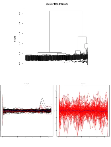
The data are combined from 5 separate groups of data, which Andrzejak et al. [17] label as A–E.

Sets A and B came from measurements on healthy individuals, while the rest are from patients who suffered from seizures, and who had later been treated with corrective surgery. The important fact about the data is that the observations from set E are all from known seizure activity.

to the known seizure activity. We also display the results of obtaining a non-hierarchical clustering by cutting the dendrogram at a given height level. We chose to form 2 groups, and display the

results also in Figure 2.2. Both groups are plotted on the same voltage range. The first group clearly has much lower voltage swings. Large voltage swings are characteristic of seizures [17]. Thus, the method has yielded a very interpretable result consistent with that known from neurobiology.

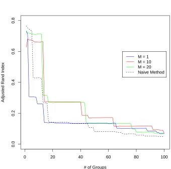
Although we apply a clustering algorithm to this data set, there is classification information available since we know which subset came from seizure activity. To evaluate the performance of our method, we use the following procedure: first, obtain a hierarchical clustering using the method described above. Subsequently, starting with 2 groups, cut the tree at various levels, and evaluate the strict clustering by computing the adjusted Rand index compared with the “true” clustering. For this comparison, we used 3 different values of M, and also compared this method to a default method. The default method was to use the same deterministic portion of our method, i.e. Ward’s method, but with a dissimilarity matrix defined by the Euclidean distance between observation vectors (an estimated L2-distance). The results of this comparison are shown in Figure 2.3. As can be seen from the results, although our method depends on the choice of mass parameter, M, for a moderate number of groups, the results are very similar between choices. For two of the choices, M =10, 20, our method outperforms the default method throughout most choices of cut point,

except for the smallest number of groups. Since, in practice, many choices of groups are likely to be explored, this gives reason to believe that our method can certainly aid in this exploration.

Using the adjusted Rand index criteria just described, we present clustering corresponding to cutting the tree at 12 groups for the model M=20. This is the point just before the drop-off in

the adjusted Rand index seen in Figure 2.3. This clustering is shown in Figure 2.4.

2.8.2

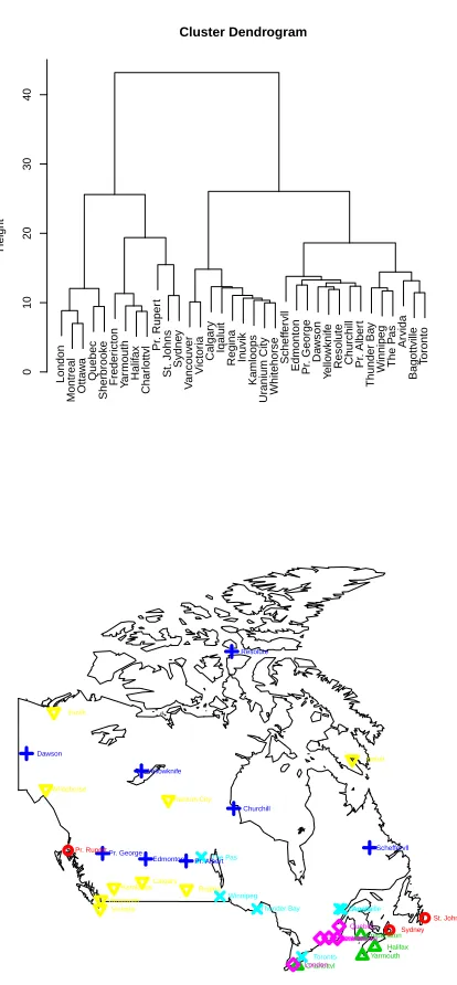
Canadian Weather Data

The next analysis involves the very popular Canadian weather data, which was obtained via the

fda

R.

35 Canadian cities. Specifically, we analyzed the precipitation data for the first 256 days of the

a naive approach based on L2-distance between observations does not nearly show as much spatial clustering. This makes this dataset “harder” than the previous EEG data, in that a naive approach to the EEG data can yield a reasonable, but less clear, description of the data. Again, this example clearly demonstrates the ability of this method to find structure between observations.

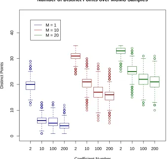
Since there is no objectively true clustering for these data, we do not compare to any other methods; however, as in the previous example, we can still analyze the effect that the choice of M has on the results. We focused on three different values, M =1, 10, 20. We present two

comparisons of the performance of the methods with these values: first, Figure 2.7 shows the approximate posterior distribution of number of distinct values for a range of coefficients in the model. As would certainly be expected, the number of groups increases as the mass parameter, M, increases because this controls the prior probability of an exact coefficient match.

To see how this affects the end result of forming a strict clustering, we show, in Figures 2.8–2.10, the end result of cutting the dendrogram obtained by Ward’s method at 6 groups. It can be seen from these plots that there is a subtle, but noticeable, effect on the results from different choices of M. Figure 2.5 shows that they generally correspond to physical proximity between the cities. This could be due to the fact that, although the cities’ climate differs in overall trends, local variations are shared, which is something our method was hoping to emphasize.

2.9

Discussion

There is an important point to note with respect to the ability of this procedure to generalize to priors other than the Dirichlet process used herewithin. In the description of the predictive distribution corresponding to the Dirichlet process, (2.11), the form suggests the possibility of a generalization to other so-called species sampling models (SSMs). SSMs are random measures for which, under certain conditions, conditionally i.i.d. sequences have predictive distributions of the same general form as (2.11) [18]. However, as pointed out by the Associate Editor, the Dirichlet process is the only member of the class of SSMs for which (2.11) will be valid when using a base measure with atoms.

of a zero value elsewhere in the hierarchy. This second option would provide an advantage that the distribution of zeroes could be chosen arbitrarily instead of being implied by the choice of SSM (which is beta for the Dirichlet process).

We would like to mention a connection between the structure of the prior and the Indian Buffet Process in the special case of the Dirichlet process prior. Typically the most important aspect of a wavelet coefficient is whether it is zero or non-zero since this respectively indicates the absence or presence of the corresponding term, and thus it is an important indicator of the sparsity of the wavelet expansion. When the quantity of interest is only the indicator that a given coefficient is zero or not, for a given observation, this can be viewed as a binary string. The Section 2.5 shows that the distribution of the total number of ones in a given string is distributed as a Poisson random variable with some rate. Because of the use of the Dirichlet process prior, the successive observations are correlated, and, in particular, exchangeable. For our prior, the probability that the (n+1)th value is 0, given that m0 out of the first n were zero, is

m0

M+n + (1−πj) M

M+n. (2.17)

Withm1=n−m0, the probability that the next value is nonzero is given by(m1+πjM)/(M+n).

If every level is considered separately, this probability coincides with that in a two-parameter Indian buffet process defined by Thibaux & Jordan [19].

However, there is a difference. The Indian buffet process is defined for equivalence classes which correspond to rearranging elements of the binary string called the left order. Since it is used mostly in latent feature models, the elements have no inherent meaning, unlike our situation, in which each element corresponds to a particular wavelet coefficient.

The assumption that the functional data are observed on an equally spaced grid of size that is a power of2 was made to use fast DWT techniques for computation. However, this restriction is

Another extension is to let the hyperparameter M also be given a prior. However, it is known that in Dirichlet mixture models the analysis can be quite sensitive to the choice of prior on M, and for exploratory purposes, running the model separately for various values of M could give a deeper understanding of the data than the results from a marginalized (over M) analysis. With a nonatomic base measure for the Dirichlet process, the standard augmentation procedure of Escobar & West [20] can be extended to the case of conditionally independent Dirichlet processes with a common concentration parameterM. However, in the present case, because of the point mass at zero in the base measure, the conditional posterior distribution of M depends also on πj, the

size of the mass at 0 in the base measure, so a slight modification of the Escobar & West [20]

procedure will be needed. Alternatively, as the conditional posterior density of M is completely explicit except for its normalizing constant and M is only a one-dimensional parameter, standard sampling procedures can be applied.

0 5 10 15 20

0.0

0.2

0.4

0.6

L2 Distance

Propor

tion of P

airs

* * * * * * * *** * * ***************** * * ** *************************************************

*

*********_****

****

0.5

0.6

0.7

0.8

0.9

1.0

Cluster Dendrogram

Height

0 20 40 60 80 100 120

−1500

−1000

−500

0

500

1000

1500

Group Size = 380

t

Voltage

0 20 40 60 80 100 120

−1500

−1000

−500

0

500

1000

1500

Group Size = 120

t

Voltage

Figure 2.2 EEG Data- Top: Dendrogram generated using the dissimilarity matrix by Ward’s method.

The stars on the margins represent observations from the fifth group (suspected seizure activity).

Bot-tom: Groups formed when the dendrogram is cut to yield 2 groups. Dashed lines are pointwise posterior

means for the observations, and solid blues lines are the pointwise group average. These figures

0 20 40 60 80 100

0.0

0.2

0.4

0.6

0.8

# of Groups

Adjusted Rand Inde

x

M = 1 M = 10 M = 20 Naive Method

Figure 2.3 EEG Data: Adjusted Rand index comparison between 3 hyperparameter choices and a

0 20 40 60 80 100 120 −1000 −500 0 500 1000

Group Size = 380

t

Voltage

0 20 40 60 80 100 120

−1000

−500

0

500

1000

Group Size = 53

t

Voltage

0 20 40 60 80 100 120

−1000

−500

0

500

1000

Group Size = 28

t

Voltage

0 20 40 60 80 100 120

−1000

−500

0

500

1000

Group Size = 3

t

V

oltage

0 20 40 60 80 100 120

−1000

−500

0

500

1000

Group Size = 3

t

V

oltage

0 20 40 60 80 100 120

−1000

−500

0

500

1000

Group Size = 2

t

V

oltage

0 20 40 60 80 100 120

−1000

−500

0

500

1000

Group Size = 4

t

V

oltage

0 20 40 60 80 100 120

−1000

−500

0

500

1000

Group Size = 4

t

V

oltage

0 20 40 60 80 100 120

−1000

−500

0

500

1000

Group Size = 4

t

V

oltage

0 20 40 60 80 100 120

−1000

−500

0

500

1000

Group Size = 10

t

V

oltage

0 20 40 60 80 100 120

−1000

−500

0

500

1000

Group Size = 7

t

V

oltage

0 20 40 60 80 100 120

−1000

−500

0

500

1000

Group Size = 2

t

V

oltage

Figure 2.4 EEG Data: Clustering the EEG data by cutting the tree at 12 groups. This corresponds to the

London Montreal Otta

w

a

Quebec

Sherbrook

e

Freder

icton

Y

ar

mouth

Halif

ax

Char

lottvl

Pr

. Ruper

t

St. Johns Sydne

y

V

ancouv

er

Victor

ia

Calgar

y

Iqaluit

Regina In

uvik

Kamloops

Ur

anium City _Whitehorse

Scheff

er

vll

Edmonton Pr. George

Da

wson

Y

ello

wknif

e

Resolute Churchill Pr. Alber

t

Thunder Ba

y

Winnipeg The P

as

Ar

vida

Bagottville

T

oronto

0

10

20

30

40

Cluster Dendrogram

Height

●St. Johns

Halifax

●Sydney

Yarmouth Charlottvl

Fredericton

Scheffervll

Arvida Bagottville

Quebec

Sherbrooke Montreal Ottawa

Toronto

London

Thunder Bay Winnipeg The Pas

Churchill

Regina

Pr. Albert

Uranium City

Edmonton

Calgary Kamloops Vancouver

Victoria

Pr. George ●Pr. Rupert Whitehorse

Dawson

Yellowknife

Iqaluit Inuvik

Resolute

Figure 2.5 Weather Data- Top: Dendrogram created from the dissimilarity matrix by Ward’s method. Bottom: Map of the cities coded by symbol in color to represent the groups formed when the dendrogram

London _Montreal Otta

w

a

Quebec

Sherbrook

e

Freder

icton

Y

ar

mouth Halif

ax

Char

lottvl

Pr

. Ruper

t

St. Johns Sydne

y

V

ancouv

er

Victor

ia

Calgar

y

Iqaluit _Regina Inuvik

Kamloops

Ur

anium City Whitehorse Scheff

er

vll

Edmonton _Pr. George Da

wson

Y

ello

wknif

e

Resolute Churchill _Pr. Alber

t

Thunder Ba

y

Winnipeg The P

as

Ar

vida

Bagottville

T

oronto

Toronto Bagottville Arvida The Pas Winnipeg Thunder Bay Pr. Albert Churchill Resolute Yellowknife Dawson Pr. George Edmonton Scheffervll Whitehorse Uranium City Kamloops Inuvik Regina Iqaluit Calgary Victoria Vancouver Sydney St. Johns Pr. Rupert Charlottvl Halifax Yarmouth Fredericton Sherbrooke Quebec Ottawa Montreal London

Figure 2.6 Weather Data- Dendrogram and heatmap created from the dissimilarity matrix by Ward’s

● ● ● ● ● ● ● ● ● ● ● ● ● ● ● ● ● ● ● ● ● ● ● ● ● ● ● ● ● ● ● ● ● ● ● ● ● ● ● ● ● ● ● ● ● ● ● ● ● ● ● ● ● ● ● ● ● ● ● ● ● ● ● ● ● ● ● ● ● ● ● ● ● ● ● ● ● ● ● ● ● ● ● ● ● ● ● ● ● ● ● ● ● ● ● ● ● ● ● ● ● ● ● ● ● ● ● ● ● ● ● ● ● ● ● ● ● ● ● ● ● ● ● ● ● ● ● ● ● ● ● ● ● ● ● ● ● ● ● ● ● ● ● ● ● ● ● ● ● ● ● ● ● ● ● ● ● ● ● ● ● ● ● ● ● ● ● ● ● ● ● ● ● ● ● ● ● ● ● ●●● ● ● ● ● ● ● ● ● ● ● ● ● ● ● ● ● ● ● ● ● ● ● ● ● ● ● ● ● ● ● ● ● ● ● ● ● ● ● ● ● ● ● ● ● ● ● ● ● ● ● ● ● ● ● ● ● ● ● ● ● ● ● ● ● ● ● ● ● ● ● ● ● ● ● ● ● ● ● ● ● ● ● ● ● ● ● ● ● ● ● ● ● ● ● ● ● ● ● ● ● ● ● ● ● ● ● ● ● ● ● ● ● ● ● ● ● ● ● ● ● ● ● ● ● ● ● ● ● ● ● ● ● ● ● ● ● ● ● ● ● ● ● ● ● ● ● ● ● ● ● ● ● ● ● ● ● ● ● ● ● ● ● ● ● ● ● ● ● ● ● ● ● ● ● ● ● ● ● ● ● ● ● ● ● ● ● ● ● ● ● ● ● ● ● ● ● ● ● ● ● ● ● ● ● ● ● ● ● ● ● ● ● ● ● ● ● ● ● ● ● ● ● ● ● ● ● ● ● ● ● ● ● ● ● ● ● ● ● ● ● ● ● ● ● ● ● ● ● ● ● ● ● ● ● ● ● ● ● ● ● ● ● ● ● ● ● ● ● ● ● ● ● ● ● ● ● ● ● ● ● ● ● ● ● ● ● ● ● ● ● ● ● ● ● ● ● ● ● ● ● ● ● ● ● ● ● ● ● ● ● ● ● ● ● ● ● ● ● ● ● ● ● ● ● ● ● ● ● ● ● ● ● ● ● ● ● ● ● ● ● ● ● ● ● ● ● ● ● ● ● ● ● ● ● ● ● ● ● ● ● ● ● ● ● ● ● ● ● ● ● ● ● ● ● ● ● ● ● ● ● ● ● ● ● ● ● ● ● ● ● ● ● ● ● ● ● ● ● ● ● ● ● ● ● ● ● ● ● ● ● ● ● ● ● ● ● ● ● ● ● ● ● ● ● ● ● ● ● ● ● ● ● ● ● ● ● ● ● ● ● ● ● ● ● ● ● ● ● ● ● ● ● ● ● ● ● ● ● ● ● ● ● ● ● ● ● ● ● ● ● ● ● ● ● ● ● ● ● ● ● ● ● ● ● ● ● ● ● ● ● ● ● ● ● ● ● ● ● ● ● ● ● ● ● ● ● ● ● ● ● ● ● ● ● ● ● ● ● ● ● ● ● ● ● ● ● ● ● ● ● ● ● ● ● ● ● ● ● ● ● ● ● ● ● ● ● ● ● ● ● ● ● ● ● ● ● ● ● ● ● ● ● ● ● ● ● ● ● ● ● ● ● ● ● ● ● ● ● ● ● ● ● ● ● ● ● ● ● ● ● ● ● ● ● ● ● ● ● ● ● ● ● ● ● ● ● ● ● ● ● ● ● ● ● ● ● ● ● ● ● ● ● ● ● ● ● ● ● ● ● ● ● ● ● ● ● ● ● ● ● ● ● ● ● ● ● ● ● ● ● ● ● ● ● ● ● ● ● ● ● ● ● ● ● ● ● ● ● ● ● ● ● ● ● ● ● ● ● ● ● ● ● ● ● ● ● ● ● ● ● ● ● ● ● ● ● ● ● ● ● ● ● ● ● ● ● ● ● ● ● ● ● ● ● ● ● ● ● ● ● ● ● ● ● ● ● ● ● ● ● ● ● ● ● ● ● ● ● ● ● ● ● ● ● ● ● ● ● ● ● ● ● ● ● ● ● ● ● ● ● ● ● ● ● ● ● ● ● ● ● ● ● ● ● ● ● ● ● ● ● ● ● ● ● ● ● ● ● ● ● ● ● ● ● ● ● ● ● ● ● ● ● ● ● ● ● ● ● ● ● ● ● ● ● ● ● ● ● ● ● ● ● ● ● ● ● ● ● ● ● ● ● ● ● ● ● ● ● ● ● ● ● ● ● ● ● ● ● ● ● ● ● ● ● ● ● ● ● ● ● ● ● ● ● ● ● ● ● ● ● ● ● ● ● ● ● ● ● ● ● ● ● ● ● ● ● ● ● ● ● ● ● ● ● ● ● ● ● ● ● ● ● ● ● ● ● ● ● ● ● ● ● ● ● ● 0 10 20 30 40 Coefficient Number Distinct P oints

2 10 100 200 2 10 100 200 2 10 100 200

M = 1 M = 10 M = 20

Number of Distinct Points over MCMC Samples

Figure 2.7 Weather Data: Boxplots of the number of distinct points in a given MCMC step for a range

of coefficients and for different values of the mass parameter,M. The coefficient numbers were chosen

0 50 100 150 200 250

−5

0

5

10

t St. Johns

Regina Uranium City

Calgary Kamloops Vancouver Victoria Whitehorse

Iqaluit Inuvik

0 50 100 150 200 250

−5

0

5

10

t Halifax Sydney Yarmouth Charlottvl Fredericton

0 50 100 150 200 250

−5

0

5

10

t Scheffervll

Arvida Thunder Bay

Winnipeg The Pas Churchill Pr. Albert Edmonton Pr. George Dawson Yellowknife

Resolute

0 50 100 150 200 250

−5

0

5

10

t Bagottville Sherbrooke Toronto

0 50 100 150 200 250

−5

0

5

10

t Quebec Montreal Ottawa London

0 50 100 150 200 250

−5

0

5

10

t Pr. Rupert

Figure 2.8 Weather Data: Clustering formed by cutting at6 groups forM =1. For each group, the

0 50 100 150 200 250

−5

0

5

10

t St. Johns

Sydney Pr. Rupert

0 50 100 150 200 250

−5

0

5

10

t Halifax Yarmouth Charlottvl Fredericton

0 50 100 150 200 250

−5

0

5

10

t Scheffervll

Churchill Pr. Albert Edmonton Pr. George Dawson Yellowknife

Resolute

0 50 100 150 200 250

−5

0

5

10

t Arvida Bagottville

Toronto Thunder Bay

Winnipeg The Pas

0 50 100 150 200 250

−5

0

5

10

t Quebec Sherbrooke

Montreal Ottawa London

0 50 100 150 200 250

−5

0

5

10

t Regina Uranium City

Calgary Kamloops Vancouver Victoria Whitehorse

Iqaluit Inuvik

0 50 100 150 200 250

−5

0

5

10

t St. Johns

Sydney

0 50 100 150 200 250

−5

0

5

10

t Halifax Yarmouth Charlottvl Fredericton

0 50 100 150 200 250

−5

0

5

10

t Scheffervll

Arvida Thunder Bay

Winnipeg The Pas Churchill Pr. Albert Edmonton Pr. George Dawson Yellowknife

Resolute

0 50 100 150 200 250

−5

0

5

10

t Bagottville Sherbrooke Toronto Pr. Rupert

0 50 100 150 200 250

−5

0

5

10

t Quebec Montreal Ottawa London

0 50 100 150 200 250

−5

0

5

10

t Regina Uranium City

Calgary Kamloops Vancouver Victoria Whitehorse

Iqaluit Inuvik

Figure 2.10 Weather Data: Clustering formed by cutting at 6groups forM =20. For each group, the

2.10

Proofs

Proof of Proposition 2.5.1. First we show that the expected number of nonzero wavelet coefficients is finite a priori. Let Aj k={βj k6=0}, k =0, 1, . . . , 2j −1 and j =0, 1, . . .. Then, as δ→0,

∞

X

j=0

2j₋₁

X

k=0

P(Aj k) =

∞

X

j=0

2j₋₁

X

k=0

ν2δ2−(1+δ)j =ν2δ

∞

X

j=0

2j2−(1+δ)j

=ν2δ

∞

X

j=0

2−jδ= ν2δ

1₋2−δ <∞,

Thus, for anyδ >0, by the Borel-Cantelli lemma, the number of nonzero wavelet coefficients is

almost surely finite. Note that, as δ→0, the expression, ν2δ 1−2−δ

−1

, converges toν2(log 2)−1

by L’Hôpital’s rule.

Similarly, for the events Bj =∪2

j₋₁

k=0Aj k, using

P(B_jc) = 2j₋₁

Y

k=0

P(Ac_{j k}) = (1₋ν₂δ21−δj)2j,

we get that

∞

X

j=0

P(Bj) =

∞

X

j=0

¦

1₋(1₋ν2δ2−(1+δ)j)2

j©

≤

∞

X

j=0

2jν₂δ2−j−δj =ν₂δ ∞

X

j=0

2−δj <_∞ (2.18)

so that the number of levels with at least one nonzero coefficient is also almost surely finite. In order to derive the Poisson limits, we apply Theorem 2 of Le Cam [21]. If X1,X2, . . . ,Xn are

independent Bernoulli random variables with success probabilities p1,p2, . . ., respectively, then

the total variation distance between the distribution of the sum, Zn =

Pn

j=1Xj and a Poisson random variable is bounded by Pn

j=1p

2

j. Specifically if Qn is the measure on N induced by

P

Xj, andQ_n∗ is the Poisson measure with rate λn=

Pn

j=1pj, with Yn∼Q

∗

n. Let kQn−Q

∗

nk=

sup_|f|≤1|E_Qn f(Zn)−EQ∗

n f (Yn)| and |f |=supx∈N|f(x)|. Then ||Qn−Q ∗

n|| ≤

Pn

j=1p

2

j. Therefore,

it suffices to boundP

j,k

P(Aj k)

2

and P

j

P(Bj)

Now,

∞

X

j=0

2j−1

X

k=0

{P(Aj k)}2=

∞

X

j=0

2j−1

X

k=0

ν2 2δ

2₂−(1+δ)2j _=ν2 2δ

2

∞

X

j=0

2−(1+2δ)j = ν

2 2δ

2

1₋2−(1+2δ) →0,

as δ→0.

Since the priors were specified independently across coefficients, the number of levels for which there is at least one nonzero coefficient (also the number of nonzero coefficients) follows the Poisson-binomial distribution, that is, the distribution of the sum of independent Bernoulli trials, but with varying parameters. Consider the sum of the squared success probabilities

∞

X

j=0

{P(Bj)}2=

∞

X

j=0

¦

1₋(1₋ν₂δ2−(1+δ)j)2j©2

≤

∞

X

j=0

2jν2δ2−j−δj 2

=ν2 2

∞

X

j=0

δ2

2−2jδ

=ν2 2

δ2

22δ₋₁. (2.19)

Notice that both the numerator and denominator of (2.19) converge to 0as δ_→0, so by L’Hôpital’s

rule the limit of the expression in (2.19) is equal to the limit of ν2

22δ 4δlog 4

−1

, which is0.

Proof of Theorem 2.6.1. Since the true vector of functions lies in _Hs

N, it is in a ball of radius B

for sufficiently large B>0. Let ε >0 and let J be the smallest integer satisfying both

N

X

i=1

∞

X

j>J

2j₋₁

X

k=0

|β(j ki),0|

2_{< ε}2_/

8. (2.20a)