Analysis of adaptive filter algorithms with an application to harmonic noise cancellation in distribution power line communications

Analysis of Adaptive Filter Algorithms with an Application to Harmonic Noise Cancellation

in Distribution Power Line Communications

by

Jin-Der Wang

Center for Communications and Signal Processing Department of Electrical and Computer Engineering

North Carolina State University

August 1985

ABSTRACT

WANG, JIN-DER. Analysis of Adaptive filter Algorithms with an Application to Harmonic Noise Cancellation in Distribution Power Line Communications. (Under the direction of Dr. Henry Joel Trussell.)

Some well-known adaptive algorithms such as the least mean squares

(LMS)

and the recursive least squares

(RLS)

algorithms are reviewed, and the properties of some newly developed fast

RLS

algorithms such as the fast Kalman (FK), the fast a priori estimation sequential technique (F AEST), and the fast transversal filter (FTF) algorithms are investigated. These adaptive algorithms are applied to the problem of harmonic noise cancellation in distribution power line communica-tions.

The fast

RLS

algorithms were derived independently, from different approaches, and no connection had previously been made. They are rederived with a unified approach, and their mathematical equivalence is shown by examining certain algorithmic quantities and initial conditions. Based on this work, an improved rescue variable is then proposed which can detect the tendency of algo-rithm divergence earlier than previously proposed rescue variables.

algorithm is derived for harmonic noise cancellation.

ii

BIOGRAPHY

Jin-Der Wang was born in Chia-Yi, Taiwan on November, 13, 1955. He received his

BSEE

and

MSEE

degrees with high honor from the National Chiao-Tung University

(NCTU),

Taiwan, in 1978 and 1980, respectively.

iii

ACKNOWLEDGEMENT

I wish to express my deep appreciation to Dr. H.

J.

Trussell, my advisor, for his supervision and guidance throughout the course of this research at all stages. This work would not be finished without his candid help and encouragement. I am thankful to the Carolina Power and Light Company and Dr.

J.

B. O'Neal for sup-porting the research. I also want to thank Mr.

J.

L. Faber for his helpful discussion during the preparation of this dissertation.

Special thanks go to my wife, my son, and my daughter for their

TABLE OF CONTENTS

LIST OF TABLES .

LIST OF FIGURES .

1. INTRODUCTION .

1.1 An Overview of Adaptive Filters .

1.2 Introduction to Adaptive Noise Cancelling ~ .. 1.3 An Overview of Power Line Communications .

1.3.1 Filtering of Power Line Noise ..

1.4 Outline of Dissertation .

2. INTRODUCTION TO ADAPTIVE ALGORITHMS .

2.1 The Least Mean Squar-es Algorithm .

2.2 The Least Squares Algorithm .

2.2.1 The Recursive Least Squares Algorithm . 2.2.2 The ~'K, F AEST, and FTF Algorithms .. 3. UNIFIED DERIVATION OF FK, FAEST, AND FTF ALGORITHMS ..

3.1 Introduction .

3.2 Review of the Fast Kalman Algorithm ..

3.3 Unification of the FK, F AEST, and FTF Algorithms ..

3.4 An Improved Rescue Variable .

3.5 Summary of Unified Derivation of Fast RLS Algorithms ..

4. CONSTRAINED ADAPTIVE ALGORITHMS ..

4.1 Introduction .

4.2 The Constrained LMS Algorithm ..

4.3 The Constrained Recursive Least Squares Algorithm ..

4.4 The Constrained Fast Kalman Algorithm ..

4.5 Summary of the Constrained Fast Kalman Algorithm .. 5. ADAPTIVE HARMONIC NOISE CANCELLATION

IN DISTRIBUTION POWER LINE COMMUNICATIONS .

5.1 In tr-od uctlon to Distribution Power Line Communications ..

5.2 The OLC Noise Model .

5.3 Simulation Conditions .

5.3.1 Corn plex Demodulation .

5.4 The Optimal Har-monic Cancelling Filter ..

5.4.1 The Demodulated DLC Noise ..

5.4.2 FIR-ALE Ilarmonic Noise Cancelling Filters . 5.4.3 (IR-ALE fla~monicNoise Cancelling Filters ..

5.5 DLC Harmonic Noise Cancellers .

5.5.1 The LMS Noise Canceller .

5.5.2 Implementation of DLC Noise Cancellers .

5.5.3 The Constrained LMS ~'ilter ..

5.5.4 Detection Error Rates of the LMS Noise Canceller . 5.5.5 Summary of the Application of the LMS Noise Canceller .

v

5.5.6 Comparison of the LMS and LS Noise Carieef ler-s 11:~

5.6 Including a liard Lirniter l lf

5.6.l Detection Er r-or Rl1tes of In clu d ing a Hard Limiter l20 5.6.2 Sumnlary of" the Addition of a Hard Limiter l:.!3

6. SUMMARY AND FUR"rHER ItESEARCH l~5

6.1 Summary of Contributions l25

6.2 Further Research 128

7. LIST OF REJ:t'ERENCES 130

8. APPENDICES 137

8.1 The Derivation of the Constrained LMS Algorithm

Using the Lagrange-Multipler Technique l37

Table 5.1 Table 5.2 Table 5.3

LIST OF TABLES

Error Count for- Unconstrained LMS Noise Canceller .. Error Count ror Constrained LMS Noise Canceller .. Error Count for Noise Canceller with/without Clipper .

Vi

LtD

112

Vll

LIST OF FlCURES

Fig. 1.1 Schematic Diagram

or

the Adaptive Noise Cancelling Concept, 3

Fig. 4.1 The Constrained ~'\i1terConfiguration 57

Fig. 5.1a A Standard DLe Time- Domain Noise Recorded in a Substation 77 Fig. 5.tb A Standard DLC Noise Spectrum Recorded in a Substation 77 Fig. 5.2a Fig. 5.2b Fig. 5.2e Fig. 5.2d Fig. 5.3a Fig. 5.3b Fig. 5.4 Fig. 5.5 Fig. 5.6a Fig. 5.6b Fig. 5.6c Fig. 5.6d Fig. 5.7 Fig. 5.8 Fig. 5.9 Fig. 5.10 Fig. 5.11 Fig. 5.12 Fig. 5.13 Fig. 5.14 Fig. 5.15 Fig. 5.16 Fig. 5.11 Fig. 5.18 Fig. 5.19 Fig. 5.20 Fig. 5.21 Fig. 5.22 Fig. 5.23 Fig. 5.24 Fig. 5.25 Fig. 5.26 Fig. 5.21 Fig. 5.28 Fig. 5.29

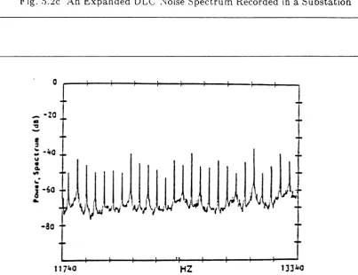
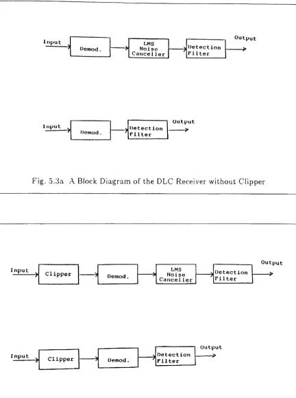
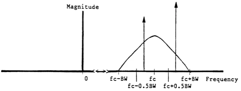
An Expanded OLe Noise Spectrum Recorded in a Substation .. An Expanded DLe Noise Spectrum Recorded in a Substation .. An Expanded DLC Noise Spectrum Recorded in a Substation . An Expanded DLC Noise Spectrum Recorded in a Substation .. A Block Diagram of the OLe Receiver without Clipper . A Block Diagram of the OLe Receiver with Clipper . A Simplified DLC Signal Spectrum before Demodulation ..

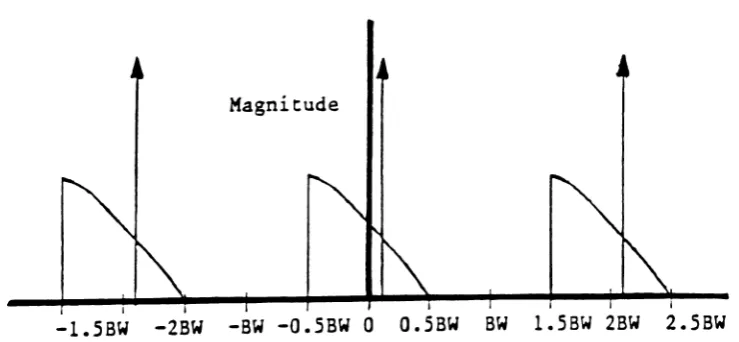
Signal Spectrum after Real Demodulation .

Signal Spectrum after Complex Demodulation .

Expanded Demodulated Signal Spectrum ..

Demodulated Signal Spectrum after Right-Shifting .. Real Reconstructed Demodulated Signal Spectrum .. The Schematic Diagram of the Adaptive Line Enchancer .

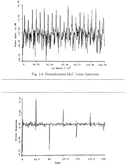
Demodulated OLC Noise Spectrum .

Adaptive Filter Response .

Adaptive Filter Spectrum ~ .

Demodulated Time Domain Noise .

Demodulated Noise Spectrum .

Time-Domain Resldual Noise .

Power Spectrum of the Residual Error ..

LMS Filter Response at the 1500th Iteration . LMS Filter Spectrum at the L500th Iteration . Adaptive Noise Canceller Requiring Signal Interruption (Method 1) . Adaptive Noise Canceller Using Out-Of-Band Noise (Method 2) . Adaptive Noise Canceller Using Out-Or-Band Noise (Method 3) ..

Constrained LMS Filter Response ..

Power Spectrum of Constrained LMS Filter .

FK Filter Spectrum at the L500th Iteration, 8 =0. L ..

FK Filter Spectrum at the 1500th Iteration, 8 =0.01 .. A DLC Noise Cancelling System with Clipper (Method 1) .. A DLC Noise Cancelling System with Clipper (Method 3) ..

Noise Spectrum After Clipping at 0.002 .

DLC Noise Spectrum after Clipping and Noise Cancellation .. Error Rates vs, Clipping Values at Different Signal Powers . Error Rates vs, Clipping Values at Different Signal Powers .

CHAPTER 1

INTRODUCTION

1.1. An Overview of Adaptive Filters

1.2. Introduction to Adaptive Noise Cancelling

The usual method of estimating a signal corrupted by additive noise is to pass it through a filter that tends to suppress the noise while leaving the signal rela-tively unchanged. The design of such filters is the major problem of optimal filter-ing, which originated with the pioneering work of Wiener and was extended and enchanced by the work of Kalman, Buey and others [48]-[53]. Noise cancelling or suppression filters can be fixed or adaptive. The design of fixed filters is based on prior knowledge of both the signal and the noise statistics. Adaptive filters, on the other hand, have the ability to adj list their own parameters automatically, and their design requires little or no a priori knowledge of signal or noise characteris-tics. Since only adaptive filters have the capability of tracking the characteristics of a changing system, we will limit our discussion to this type of filter.

[1]-5 (n)

=

Si(n) + n

1 (n) error output

".I

S. (n)

~

- - - -... Fil ter

Prediction output - . , . . . - - '

Si(

n)

is the signal to be detected.

nl(n)

and

n2(n)

are noises which are uncorrelated with the signal but correlated

with each other.

Fig. 1.1 Schematic Diagram of the Adaptive Noise Cancelling Concept

[2], the RLS algorithm [75], and investigate the properties of some newly developed fast RLS algorithms such as the fast Kalman (FK) [54]-[58], the fast a priori esti-mation sequential technique (F AEST) [59]-[60], and the fast transversal filter (FTF) algorithms [61]. These fast algorithms were derived independently, from dif-ferent approaches, and no connection had previously been made. We will rederive these fast algorithms with a unified approach [62], and show their mathematical equivalence by examining certain algorithmic quantities and initial conditions. Based on this work, we will also propose an improved rescue variable which can detect the tendency of algorithm divergence earlier than previously proposed

4

noise reduction for distribution power line comrnunication systems. To save corn-putations, we will also derive algorithms which constrain insignificant filter taps to zero for the adaptive harrnonir noise cancellation rase. These constrained adaptive algorithms can also be applied to different problems such as long-term prediction in adaptive predictive coding for speech signals and multipath propagation channel correction.

1.3. An Overview of Power Line Communications

Within the broad area of power line communications, there are several dif-ferent applications [63]-[67], such as load management, remote meter reading, and distribution equipment monitoring and control, which can use power lines as a medium for communications. The distribution power lines are also being used for voice-grade communications in remote housing areas, and in the home for local control and monitoring of appliances. Power line communication is implemented by injecting a signal onto the existing transmission or distribution power lines owned by the public utilities. This signal is then received elsewhere on the power

system, and the signal is acted upon.

Power lines are traditionally a very noisy environment in which to transmit

signals, and are divided into two broad categories by the utility industry: transmis-sion and distribution power lines. Transmistransmis-sion power lines are these which carry power from the generator to the distribution substations, where they branch out to

All manner of devices are connected to the distribution power lines. These devices, such as light dimmers, universal motors and other common household appliances [68]-[7~], might contain switching devices which can inject large voltage/current spikes anywhere onto the distribution power lines. The large spikes, which are generated by switching the loads on the lines, are synchronous with the fundamental 60 Hz power signal such that they appear as 60 Hz harmon-ics. Generally these harmonics are not very large compared to the 60 Hz funda-mental. However, when it is desired to transmit signals over the distribution power lines, these harmonics can be a serious problem, especially when signals are transmitted over a distance long enough to cause substantial attenuation of the signal, thus decreasing the signal-to-noise ratio. The signal transmission can become very difficult, if the harmonic noise is not removed from the line by some

type of filtering technique.

Transmission power lines do not have consumer or industrial switching dev-ices connected to them because they are high voltage lines llsed exclusively to carry power from the generator to the distribution substations. They are therefore much cleaner than distribution power lines, and make a better transmission medium. The current interest in power line communications is directed toward the distribu-tion power line so that the utilities may access individual homes and commercial

6

1.3.1. Filtering of Power Line Noise

7

designed to take these variations into account [73]"

Since the harmonic noise is man if'est.ed by large spikes in the time domain, it IS natural to try to attenuate their effect by preprocessing the signal with a hard

I"t d 1"" (" I" If)

amp I u e irruter (' ipper . Many DLC~ systems currently in use employ hard limiters to reduce this type of noise prior to detection of the signal. We will show that an adaptive noise cancellation filter can be used effectively in tandem with hard limiters

[73]-[74].

1.4. Outline of Dissertation

In Chapter 2, we review some well-known and some newly developed adaptive algorithms. In Chapter 3, we describe a unified approach deriving the fast RLS algorithms, such as the F'K, F AEST, and FTF algorithms, and shows their mathematical equivalence by examining the algorithmic quantities and initial con-ditions defined in this approach. In Chapter 4, we develop constrained adaptive algorithms for applications such as the long-term prediction of adaptive predictive coding for speech signals, the harmonic noise cancellation of distribution power line communications, and multipath propagation channel correction. In Chapter 5, we describe the adaptive cancellation of harmonic noise in the distribution power line communications. It is shown that the adaptive noise cancellation filter can be used effectively in tandem with hard limiters. In Chapter 6, we summarize impor-tant results achieved during the course of this research and propose some topics of

8

CHAPTER

2

INTRODUCTION TO ADAPTIVE ALGORITHMS

2.1. The Least Mean Squares Algorithm

The least mean squares (LMS) algorithm [1]-[3] adaptively computes a filter which minimizes a mean squared error. This algorithm is different from the least squares (LS) approach which minimizes a weighted sum of squared residual errors. The LS approach will be discussed in the next section. It can be noted that the mean squared error is a quadratic function of the filter parameters, which can be pictured as a concave hyperparaboloidal surface in N-space

[1].

Adjusting the filter parameters to minimize the mean squared error can be done by "descending" along this surface until the nbottomn of the paraboloid is found. The steepest-descent method can be used to do this. The LMS algorithm is derived by using this method. A sketch of the development of the LMS equations is given below. The prediction error is defined as:

e(n)

=

d(n) - y&(n)wN(n-1),

(2.1)

9

* -

R-

1

WN - yy ryd' (2.2)

where

R

yy is the autocorrelation matrix of y and Tyd is the crosscorrelation vector between y snd d. The iterative procedure of (2.2) is updated by taking the present filter value and adding a change to it proportional to the negative of the gradient

wN(n)

= 'wN(n-l) - JiV_w

E [e(n )2],

where Ii is the step size, and V is the gradient operator.

(2.3)

Note that

(2.3)

actually implements the steepest-descent algorithm and relies on finding the gradient of the mean squared error with respect to

wNCn).

How-ever, the mean squared error is unknown. Widrow

[1]

approximated the mean squared error by the instantaneous squared error and called this algorithm the LMS algorithm. It can be shown that after the approximation

(2.2)

reduces to

wN(n)

=

wN{n-l)

+

2li

e{n )YN(n ).

It can also be shown that Ii must satisfy the inequality,

(2.4)

o

<

Ii

<

l/~max ,

to assure algorithm stability, where ~max is the maximum eigenvalue associated ith

R

It is well-known that the eigenvalue l:maxsatisfies the inequality,

WI

sv:

~

~max ~ trace

[R

yy ]' where

(2.5)

N T

trace

[R

_{yy ]}

=

~~i

=

E[YN(n)YN(n)].

i=l

10

slow time-variation of input statistics. To assure algorithm stability, f-L must be changed according to input statistics.

A

modified

LMS

algorithm, the so-called normalized LMS (NLMS) algorithm [2], is used in practice for this purpose. Let us define the cumulative instantaneous signal power, Pin

(n),

where

(2.6)

1

Then we can replace fJ. by so that the step size adjusts automatically Pin

(n )

according to the input signal power. The NLMS algorithm is thus written as:

(2.7)

11

2.2. The Least Squares Algorithm

Instead of minirnizing the mean-square error, the LS approach minimizes a weighted sum of squared residual errors defined as:

n

~(wN(n))

=

2:

a(-n-i)[d(i) -

wJ(n)YN(i)]2,

i=O

(2.8)

where

{a(0),a(1),a(2), ...}

is a sequence of the "forgetting" weights. Two common choices for this weight sequence are

a

(i)

= AZ

• forO

<

A

<

l,

and

{

~'

for

o

< z· :5 N[-l

a{i)

==

otherwise,

0

(2.9a)

(2.9b) where l\ is the" forgetting factor". The first choice is called an exponential weight-ing. The effect of the past samples fades out exponentially. The second choice is called sliding window forgetting. It uses only the last N{ samples to do the adaptive

processing and those samples are weighted equally. Both weighting schemes can be used to handle slow time-variation of the input statistics. The exponential weight-ing scheme is commonly used in digital signal processweight-ing applications, and it will

be considered here.

The

LS

algorithm can be summarized as follows:

(2.10) where

12

TN(n)

=

A

TN(n - 1)+ YN(n )d(n ).

(2.12)

Here,

R

NN is a weighted short time estimate of the input signal autocorrelation

matrix and rN is a short time estimate of the correlation vector between YNand d.

Using the matrix inverse lemma

[76]

on

(2.11)

and grouping the intermediate

terms properly yields a form similar to the LMS algorithm:

(2.13)

Comparing (2.13) to

(2.3)

we see that the constant step size in the LMS

algo-rithm has been replaced by the inverse of a matrix

RNN{n).

Here,

RN"J(n)

essen-tially offers more than the simple step size in the LMS algorithm or the simple

power normalization (varying the step size inversely with signal power) in the

nor-malized LMS algorithm. It adjusts the adaptation in each eigenvector direction by

the signal power in that direction. Thus convergence becomes less sensitive to

sig-nal statistics.

Since it takes O(

N

3 ) multiplications to compute the inverse of

R

NN{ n)

directly by Gaussian elimination and backward substitution, current technology

makes this direct solution impossible for real-time signal processing, where N is

struc-13

ture of

R

NN · We will introduce these fast algorithms in the following sections.

2.2.1. The Recursive Least Squares Algorithm

The recursive least squares algorithm is used to reduce the number of compu-tations to O(lV2) multiplications per iteration. We will present this algorithm without detailed derivation. The reader is directed to

[7,5]

for detailed derivation.

wN(n)

=

wN(n-l)

+

kN{n)e(n)

RN"J(n-l)YN(n)

k_{N (}

n)

=

~

+

yJ(n)RNrJ(n -l)YN(n)

RNJ(n)

=

l.[RNJ(n-1) - kN(n)yJ(n)RNJ(n-1)]

~

Here, k_{N (}n ) can be rewritten as:

(2.14)

(2.15)

(2.16)

kN(n)

=

RNJ(n)YN(n),

(2.17)

where kN (

n)

is usually referred to as the Kalman gain vector because of the

simi-larity of (2.14-2.16) to a Kalman filter [50]-[51].

2.2.2. The Fast Kalman, FAEST, and FTF Algorithms

In the past few years, fast algorithms further exploiting the special properties

of

R

_NN have been proposed, with the cost of computing the Kalman gain vector

reduced to O(N) multiplications per iteration. They can be classified into two

categories by their approach to the solution. One is the fixed-order (Kalman) type

least squares algorithm, and the other is the lattice (ladder) or variable-order type

algorithm. The discussion here will be limited to fixed-order type least squares

14

t5

(~HAPTElt :J

UNIFIED DERIVATION OF f'K, FAEST, AND FTF ALGORITHMS

3.1. Introduction

The three fast fixed-order RLS algorithms, the FK, F AEST, and FTF algo-rithms, exploit the property that

R

_{NN (}n -

1)

is closely related to RNN('n); most of the elements of RNN(n) are available from R_{NN ( n}

-1).

Recognizing this property, Morf, Ljung, Kailath, and Falconer

[54]i-[56]

were able to reduce the computa-tional complexity of updating the Kalman gain vector to 8N multiplications per iteration. This algorithm is now commonly referred to as the fast Kalman algo-rithm. It was derived using somewhat complicated matrix manipulations. Samson [57] later rederived the FK algorithm from a vector-space viewpoint. Recently, Carayannis, et al. [59]-[60] introduced the F AEST algorithm which requires only 5N multiplications per iteration. This complexity reduction is achieved through a different definition of the Kalman gain vector, the "alternative" Kalman gain vec-tor, introducing an "a posteriori error" formulation of the problem in contrast to the "a priori error" formulation in the FK algorithm

[,')4]-[58].

It was also derived using complicated matrix manipulations. Motivated by the work of Carayannis, et aI., Cioffi and Kailath [61] derived independently another 5N algorithm they called the FTF algorithm, from a vector-space viewpoint.

L6

algorithms. It is the pu rpose of this chapter to demonstrate a unified derivation of these three algorithms frorn a vector-space viewpoint. This unified derivation is achieved by examining the redundancies existing in the ~'(( algorit h m. Therefore, in Section 3.2 Sarnsons derivation of the FK algorithm

[,j 7]

will he reviewed and the redundancies will be pointed out. In Section 3.3. the f"AEST and FTF algo-rithms will be derived

by

simplifying the

FK

algorithm. This is achieved through careful examination of certain quantities defined for this unified derivation.

By

examining these quantities and the initial conditions of these fast algorithms, we will demonstrate their mathematical equivalence; the differences in performance result from the finite arithmetic effects due to the particular implementation. In Section 3.4, an improved rescue variable will be proposed. We believe that this uni-fied derivation can result in a better understanding of these fast algorithms.

3.2. Review of the Fast Kalman Algorithm

In the past few years, the vector-space approach has been demonstrated to be effective in deriving fast algorithms. Therefore, this approach will be adopted here. The derivation of the FK algorithm frorn a vector-space viewpoint has been dis-cussed in detail in

[,57].

A review of this work will be given here in order that the

reader may gain insight into the concept of the unified derivation.

The input signal is assumed to be "pre-windowed". That is y(n)===O, for n~O.

YM(n)

=

[y(n)y(n-1) '"

y(l)a ... alT,

17

(3.1)

where M is an arbitrarily large integer

(M>

>

n). This fixes the dimensionality of the vector space by appending zeros to the end of the input vector and helps to avoid some abiguities which can arise when time advances. These zeros have no effect when inner products are defined. The data matrix which contains the N most recent input vectors is defined as:

YMN(n)

=

[YM(n)

YM(n-l) .... YM(n-N+l)].

(3.2)

The vector space to be dealt with is a subspace of RM , with the M dimensional vector space defined over real numbers. The basis vectors for this subspace are the columns of Y

MN( n).

Before deriving the FK algorithm, operators useful in the vecto- space approach will be defined. Although the introduction of these operators might seem arbitrary now, their usefulness will become clear later. For simplicity, the forgetting factor Ais assumed to be unity. The case with variable Acan be derived similarly.

The pinning vector

,c

The

Mxl

pinning vector is defined as:

IT

=

[1

a a a·· ·

O]

T.

(3.3)

The product of

a

T with any time-dependent

Mxl

vector reproduces the most recent time component of this vector.

The shifting matrix,S

L8

o

1 0 . . 0 . 010

s=

_{. . . 0 1 0}

. () 1

o . . . .

0

(3.4)

The product of S with any time-dependent Mxl vector shifts this vector one sam-pie back. This property also holds for any time-dependent rnatrix with ~1 rows. As examples,

SYiW"N (n) == [Yi\! (n -

1)

YM (n -

2) ...

YM (n - N)] == YM N (n - 1)

The residual oper-ator .P" ·

s

YM (

n)

=

[y

(-n --

1)

Y

(n --

:2 )

y(l)

a ...

o]T

== YM(n-l)

(3.5)

(3.6)

The NlxM operator P

y

is defined as:

(3.7)

where I is the MxM identity matrix. One can easily verify that

PyP y

==

Py

and

P

y

==

P

y

T; thus

P

y

is an orthogonal projection operator. As a shorthand notation, we define

PyO(n

-1)

=

po

_{: YMN(n - L)}'}

where MN is the dimension of Y.

A physical in ter pret.at.ion of this residual operator,

P

y(

n

-1),

can be given. The product of

P

y(

n -

1)

with the new input vector YMCn) yields a Mxl residual

error vector:

e~(n)

=

PY(n -l)YM(n).

(3.8)

(3.9)

19

combination of the columns of Y.WN('n

-1)

which are the basis vectors for the sub-space of time n-1. We can verify this by substituting the definition of the residual operator of (3.7) into the above equation. This yields

e~{n

)

=

{I -

YMN(n-l)[Y~N(n-l)YMN(n-l)]-lY~N(n-l)}YM(n)

=

YM{n) -

YMN(n-l)AN(n),

where

AN(·n)

can be considered as the forward prediction filter obtained by

minim-The order updating formula

The order updating formula relates an operator to a new operator obtained by expanding the dimensionality of a subspace. The incorporation of a new basis vec-tor into the old orthogonal projection operavec-tor is a direct sum of the old projection operator and the orthogonal contribution of this new basis vector.

Pu,V

=

P y - pyU[UTpyUrlUTpy,

where V is a matrix and U is a vector, with the same number of rows. The time updating formula

(3.10)

This formula relates an operator to a new operator, of same dimensionality, when time advances. When a new input vector becomes available, the oldest input vector is discarded; thus the basis vectors of the vector space change, and the projection

operator should be updated accordingly. The formula holds as long as

58

T

= [ _

oo

T .

The time updatting formula is

P

y

=

S r PSyS

+

P,?

TU[Ur

P~,ul

IU7'

Pr.

The prediction operator,(JrJ

Qy

= [ -

Y(

}"T~~T.~,}~) 1}/T.STS.

As a shorthand notation, we define

Qy(n-l)

= QfYMN(n-l)}~

where MN is the dimension of IT.

20

(3.12)

(3.13)

A physical interpretation of the prediction operator,

Qy(n

-1),

can be given.

The product of

Qy(

n

-1)

with the new input vector YM(

n)

produces a prediction error vector:

(3.14) The new input vector is best predicted (in the least squares sense) by a linear corn-bination of the columns of

Y

MN(n -

1)

which are the basis vectors for the subspace of time n-l. We can verify this by substituting the definition of the prediction operator of (3.13) into the above equation. This yields

EM{n)

(I -

YMN(n

-1) [

YJN( n -1)8 r SYMN(n

-1)]

-1

r,~N(n

_1)S1' S }YM(n)

~ (3.15)

YM(n) - YMN(n- 1)

[~r,~N(n

_{-2)YMN(n 2)}

]-1

Y,~N(n

-2)YM(n -1) YM{n) - YMN(n l)ANCn

--1),

where AN{n

-1)

was defined in (3.9). Examining (3.9) and (3.15), we find that

they resemble each other. The only difference is the time indices of AN (

n).

This

~l

between QO and

po

is

rrTQy

=

[(r

TpyfTr1fTTP

Y.

(:3.l6)

where ITT

P).-a

is a scalar. Samson [8] did not take full ad vantage of this relation-ship in deriving the fast Kalman algorithm; however, it will be

or

substantial value in the unified derivation of the

F'K,

F

AES"r,

and FTF algorithms.

The parameter operator,K

The parameter operator K is closely related to the Kalman gain vector. The Kal-man gain vector is the product of K with the pinning vector.

The NxM parameter operator Kr is defined as:

Kv

> (yTy)-lyT.

The order updating formulas

These two formulas relate

K

u,

v to

K

u

and to

K

v' respectively.

[

K

U ]

[-KuV]

K

_v,V

=

0

+

1 (

V

T

Plj

V)-l

V

T

Plj,

where U is a matrix and V is a vector, with the same n urnber of rows.

K_{V,V -}-

[0

_KV

1

+ [

_{- K}1_VU](UTPO[!)-L[!TPO

v

_v'

where V is a matrix and U is a vector, with the same number of rows.

The time updating formula

The formula relating K_{S Y} to Ky is given as follows:

K y

=

KsyS

+

K yfTfTTQY.

(3.17)

(3.18)

(3.l9)

In order to conform with the not.at.ion of the vector-space approach, kN(n) in (2.17) will be rewritten using the definitions of YM(n) an d }r_{Af N}(n) from (;~.1) and

(3.21) It can also be expressed in terms of the parameter operator K, and the pinning vee-tor:

(3.22) When time advances, the only change of the basis of the current subspace is the newest entering input vector and the oldest discarded input vector. Recogniz-ing this property, the FK algorithm was derived dealRecogniz-ing with these two input vec-tors. Therefore, the reader can expect the involvement of a "forward predictor" (predicting forward the newest entering input vector), a "backward predictor" (predicting backward the oldest discarded input vector), and some associated error quantities. Let us now define certain quantities that will be useful in the

deriva-tion of a recursive computaderiva-tion of

k

_{N (}

n).

e'(n)

==

yZ;(n)Py(n

-l)rr

e(

n) == y

J(

n )

Q

y(

n - 1

)(T

r(n) ==

yI;(n-

N)Py(n)a

-y(n)

=

yl;(n-N)Qy(-n)fT

AN(n)

==

Ky(n -

L)YM(n)

DN (n) == K y (n )YM (n --N)

forward residual error

forward prediction error

backuiar d residual error

backward prediction error

forward predictor

backward predictor

E(n)

=

YA~(n)Py(n

I)YJ,(n) forward residuul power (3.29)

F(n)

=

y.[,(n-N)PY(n)Y\f(n

N) backward residual power (3.:30)

The quantities defined in (:-~.:2S) and (~.:30) will not be used in deriving the FK algo-rithrn. However, they \\'i11 be needed in deriving the F~-\ES'rand F'TF algorithms.

'0/e also need to introduce

kN+L(n),

the so-called "extended Kalman gain vee-tor." Replacing Nand Yin (3.22) by N+l and Yi\tf(,V+-l)(rt) respectively, we obtain

k,V+l('n)

== K{Y;'vl(N_II(n)}u, (3.31)

where 0r+ 1 indicates the "extended" dimensionality. Now (3.19) allows us to relate k/V+-L{n) to k~v(n-l). Postmultiplying (3.19) by (J, with

U

==

YM(n)

and

v

==

Y.\tf:V(n -1), yields

(3.32) Here, k.'V __L(n) is partitioned into:

kN+1(n)

=

[~~~)],

(3.33)

where

mN(n)

is a Nxl vector and ~(n) is a scalar.

We

will now relate

kN+l{n)

to

k_N(

n).

Postmultiplying (3.18) by rr , with U = Y

MN( n)

and V =

YM( n - N),

yields

where

[

kN( n ) ]

[D,v(n)]

o

+

I

jJ..(

n),

(3.34)

-L T 0

~

jJ..(n)

=

[YM(n -N)TPY(n)YM(n

N)]

YM(n-N) Py(n)rr

=

F(n)

(3.35)

24

(3.36)

However, before this equation can be evaluated. the recursive l'or ms for updating E(n).

e'(n), A.dn),

E(n),

-y(n).

and DN(n) should be provided.

The recurs! ve form of

E(

n) can be obtained by prernultiplying (3.1S) by

IT

T.

E(

n )

=

(TT{Y:wCn) --

}TMJvCn-l)/t.lv(n---L)}

=

yT(n) -

y,~(n-l)itN(n-l)

(3.37)

The recursive form of 4-!N call be derived as follows. Using the time updating formula of the K operator in (3.20), postmultiplying by

YM( n),

we obtain

Ky(-n

-l)YM(n)

=

Ky(n -2)YM(n

1)

+

Ky(n

--l)rrrrTQy(n --l)YM(n).

Substituting the definitions in (3.27), (3.22), and (3.24) yields

(3.38)

The recursive form of e

(n)

can be obtained by premultiplying

(3.9)

by ITT:

e'(n)

= (TT{YM(n) - YMN(n-l)ANCn)}

=

yT(n) -

yJ(n-l)AN{n).

(3.39)

The recursive form of E(

n)

ran be derived as follows. Using the time updating formula of (3.12), premultiplying by Y.~(

n)

and postmultiplying by YM(

n),

we

obtain

yJ(

n

)P

y(

n

-l)YM(

n)

=

yJ(

n)8

TPfSYMN(n h l)}SYM(

n)

+

yJ(n)PY(n

-l)a[uT

PY(n

l)a]laT

PY(n --l)YM(n).

yZ;(n)P

y(n-1)YM(n)

=

yZ;(n-1)P

y(n-2)YM(n

"'1)

+

YZ;(n)P},(n l)mrT(j}-(n I)!hr(n).

Substituting the definitions in (:3.:23), (3.24), and (;L:2H) into the above equation yields

E(n)

==

E(n-l)

+

e'(n)e(n).

The recursive Ior m of )'(n) can be derived as follows. Using derivation similar to that leading to (;_3.37), we premultiply and postmultiply QO by aT and

YM(n - N), respectively, and substitute the definition of D_N(n) in (3.28). This yields

(3.41 ) The recursive form of D_N can be derived as follows. Using the time updating formula of the K operator in (3.20), postmultiplying by YM(n -

N),

we obtain

Ky(n)YM(n N)

= Ky{rt -

L)YM(n

-N-l) -

Ky(n)(TuTQY(n)YM(n--;·V).

Substituting definitions in equations (3.28), (3.26), and (:3.22) into the above yields

(3.42) Equations (3.42) and (3.36) can be used to simultaneously solve for D_{N (}n) and

k_N(

n)

in terms of previously computed quantities. This yields

DN(n-

L)

+

mNCn)~(n)

DN(n) = 1 - /-l(n)-y(n) .

Substitution of (3.43) into (:3.;36) willgive k_{N (}n).

(3.33) The important results of the preceding derivation are summarized below.

Summary of the FK Algorithm

e(n)

=

y(n) - yJ(n

-1)A,y(n -1)

(3.:~7)

AN(n)

=

AN(n -

1)

+

k,v(n

-1)e(n)

(3.38)

e'(n)

=

y(n) - yJ(n --

L)Aj.y(n)

(

3.39)

E(n)

=

E(n -1)

+

e'(n)e(n)

(3.40)

k,v+-l(n)

=

[kN(~-1)

I

+

[-A~(n)

I

[E(n)r1e'(n)

(3.32)

Partition

[~~~)

I

)'(n)

=

y(n-N) - yJ(n)DN(n-t)

(3.41)

D

N (

n -

1)

+

mN (

n ))'(n )

DN{n)

=

(3 43)

1 -

fi(n)),(n)

·

kN{n)

=

mN(n)

+

DN(n)lJ.(n)

(3.36)

The initial conditions are as follows: AN(O) == ON, DN(O) == ON' kN(O) == ON, and £(0) = 8>0 to assure stability. The joint process can be updated by the following recursion:

where

e(n)

=

[d(n) -

yJ(n)·wN{n

-1)].

3.3. Unification of the F K, F AEST and FTF Algorithms

We will derive the F AEST and FTF algorithms by examining the

27

careful examination of the initial conditions, t.hp three algorithms are shown to be mathematically equivalent. The uu mer ical im pleruentation is all that makes them appear different.

A. Efficient update of the forward prediction error

Let us recall a very important relationship between Q0 and

P"

,(3.16),

(TT

Q?

=

[a

T

Pya] --

L(TT

P

r.

This relationship will playa central role in our unified derivation of the FK, F~t\EST, and FTF algorithrns. We define u(

n)

as:

a(

n)

=

ITT

P

y(

n

)a. We define ~(n) as:

(3.44)

(3.45 ) Examining the ratio of the forward residual error of (3.23) to the forward predic-tion error of (3.24), we find that

e'(n)

=

E(n)O'.(n-l).

(3.46)

[f a(

n)

can be updated efficiently, the N multiplications for computing the for-ward prediction error of

(3.39),

can be replaced by one multiplication. Since ~(n) is the reciprocal ofa(

n),

(~~.46) can also be rewritten as:

e'(n)

=

E(n)

(3.47)

f3(n --

1)

28

updates ~(n) is the F AEST algorithm. Two intermediary quantities which will be used in deriving efficient updates of cx(

n)

and ~(n) are defined below. The "extended" 0.(

n),

0.'

(n),

is defined as:

a'(n) -

crT

po

- {YM(N_I)(n)}(T

The" extended" ~(n),

s

(n),

is defined as:

Q. ' (

n) - [a

TP O ] -1 tJ - {YM(N-I)(n)}(J"

Note again that

N+l

indicate the extended dimensionality.

(3.48)

(3.49)

Since the recursion of the backward residual power F(n) will be used in the following derivation of the efficient update of the backward predictor, we will now derive it. Using derivation similar to that leading to (3.40), the recursive form of F(N) can be derived. Premultiplying and postmultiplying the time updating for-mula of (3.12) by

y};(n-N)

and

YM(n-N),

respectively, yields

F (n)

=

F (n -

1)

+

r (n)~( n ).

B. Efficient update of the backward predictor

(3.50)

If the dependence of

k

_{N (}

n)

on

D

_{N (}

n)

shown in

(3.42)

can be broken, the extra N divisions computed in

(3.43)

can be eliminated. This dependence can be broken by substituting D_{N (}

n)

defined in

(3.42)

into

(3.34).

This yields

[

kN(n ) ]

[-DN(n-l)-kN(n)~(n)]

k

_N

+1(n )

= 0

+

1

lJ.(n),

[

kN(n)(l -~(n )J.L(n)) 1

[-DN(n-l)]

(3.51a)

k

_N

+1(n)

= 0

+

1

lJ.(n).

29

can simplify 1-~(n)J..L(n) to

1 -- -y (n )/-l(n)

=

F (n-

1)

F(n)

It will be shown in (3.62) that

cdn)

=

U~(n) (3.51a) by

a/(n),

we obtain

(3.S1b) Using this fact and dividing

Here,

k~

+1(n) is partitioned into:

[

m~( n ) l

k~+dn)

= /-l'(n)

Equating the rnatched vectors of (3.52) and (3.53) yields

(3.52) y( n)

F(n-l)'

(3.53)

k~(n)

=

m~(n)

+

/-l'(n)DN(n-l) (3.54)

If

k~(

n) is updated instead of _kN(n), the evaluation of

k~(

n) no longer depends on

D

N (

n).

The backward predictor,

D

N (

n),

can now be evaluated, using only N

mul-tiplications, by

DN(n)

=

DN(n -1)

+

k~(n)r(n)

where we use the backward residual error defined in (:~.26).

c.

Efficient update of the backward prediction error

Examining (3.52) and

(3.,5:3),

we find that

'Y(n)

can be updated by

'Y(

n)

= f.L' (

n

)F

(n -

1).

(3.56)

~o

backward prediction error of (:L 11) could he replaced by one multiplicnt.ion. D. Efficient update of the backward residual error

Although the backward residual error is not available in the

FK

algorithm, it is needed here for updating F'(n). I-Iowever, since the ratio of the backward resi-dual error to the backward prediction error,

u(

n),

is available, the evaluation of r(n) can easily be computed. This ratio can be found by examining (3.25) and (~1.26).

r(n) ==

'"Y(n)u:(n)

It can also be rewritten as

r(n)

=

~.

~(n)

(3.57)

(3.58)

In order to obtain these efficient updates, the update of

a

TPya must be pro-vided. Different updates of

a

T

Pya

will result in the F'TF and FAEST algorithms.

Update the FTF algorithm

If we choose to update ITTPya directly, the resulting algorithm will be the

FTF algorithm. Postmultiplying (3.13) by IT and premultiplying by aT, with

U

=

YMN(n-l) and V == Yf\;,(n),yields

o:'(n)

- Tpo IT

- IT {YMN(n-l),YM(n)}

=

rr

TPY(n -

l)rr

(~.59)

-

rrTPY(n-l)YM(n)[y~(n)PY(n-

I)YM(n)]

ly~(n)PY(n-

l)rr

e'(n)

'( )

=

u(

n -

l ] - E

(n) en.

, E(n-I)

ex

(n)

=

l't(n - 1 ) .

E(n)

(:3.60)

Postmultiplying (3.13) by IT and premultiplying by (TT. with L' == _Y:\JN(_n and V == r",\;f,V(n), yields

a'( n)

== rrTpo

{YMN(n - .V},Y.\fN(n)}IT

=

aTP}~(n )a

- ITT

PH

n

)YM(

n -

:V)[Y.!t(

n -- N)Pf·(n

)YM(

n - N)rl

Y~(

n - N)PY(n)IT

=

u(n) -

r(n) r(n).

F(n)

Substituting (3.S0)and (3.57)into (3.61) yields

, F( n)

Cl( n)

= a (n) . .

F(n

-1)

Substituting

(;3 ..56),

(3.50),and (3.57)into (3.62)yields

u(n)

=

u·(~).

1 .- 'Y (

n)a (n)

J.l

(n )

Substituting (3.60)into (3.63) completes the updating formula of

a( n).

Update the FAEST algorithm

(3.61 )

(3.62)

(3.63)

If we choose to update [rrT

Pya] .

L, the resulting .rlgorithrn will be the F AEST

algorithm. This term was defined as ~ and is the reciprocal of o , Since

u(n)

and

~(n) are updated differently, they have different numer ical properties [6] where

finite arithmetic is considered. Taking the inverse of

(:3.59)

and applying the

~'

(n)

=

[UT

P{YMN(n-l),YM(nj}U] I

=

[uTPy(n-l)ar l - [cr1'P

y

( n

L)(Trl[--ITTPy(n--L)YM(n)]

([Y,!t(n)PY(n-l)YM(n)]

+

[y,[,(rt)Py(n-l)a][uTPy(n-L)<J]-1

[- crT

P

Y(

n - L)YM (n )]} - I

Y

.~(

n )

P

Y(

n - L)u[ITT

P}-(

n - l)a

r

l

=

[3(n-L)

+

cr1'QY(n-l)YJf(n)[E(n) - e'(n)E(n)rlyl;(n)QY(n-l)a

=

[3 (n --1)

+

E (n ) E (n ). E(n-l)

Using the same procedure on (3.61), we obtain

[3'(n)

=

[3(n)

+

~dn}

-y(n). F(n-l)

Substituting (3.56) into the above equation yields

(3.64)

(3.6Ej)

(3.66) Since we now must update k~+l(n) instead of kN+1(n), (3.32) and (3.38) should change accordingly. Recall that

AN(n) == /I_N(n-L)

+

kN(n-l)e(n) and

[ 0

I [

1

I

- l

I

kN+1(n)

=

kN(n-l)

+

-AN(n)

[E(n)]

e

(n)

Substituting A_{N (}

n)

defined in (3.38) into (3.32) yields

I

[0

I

[

L

1

E(

n )

K

N+1 (n ) =

k~(n-l)

+-AN(n-l)

E(n-L)

Equation (3.38) is also changed accordingly. It becomes

(:3.67)

The alternative Kalman ~:Jill vector

[,)9]-[60]

isdefined as:

ka(n)

=

[Y-.~N(

n -

L)

Y._UN(n

1)1

I

Y.fr(

n ).

We now prove that

k~(

n) is ('quivalent to the alternative Kalman gain vector. Similarly, the equivalence of k,~/-I (n) and the "extended" alternative Kalman gain vector can he proven.

Applying the matrix Inverse lemma [76] to yTST;-,'}to" and noting that ."'.~'T == I - (TITT yields

[yT.<."T.';;'Tj-1 = [y-TYr l

+

[y'TY-rly-Ta[aTPyarLO'Ty["VTYrl Postmultiplying (3.69) by yz.(

n),

with Y == YMN(

n),

yields

k_a

(n)

==

[Y~N(n

-1) Y

MN{n

-l)]-lyZ(n)

=

[Y~N(n)"V

MN( n)r

ly~(

n)

+

[}r~N(

n)

y-MN(n)rI YMN(n)O' T

[aT

Py(n

)a]- laT

Y

MN(n)[

YltN(

n)YMN(n

)]-1

yI;N(

n)a

==

k,v(n){l

+

[aT

P

y(

n )a] -LaT

Y,MN(

n)[rO"J~N(n)

Y

MN(n)] - 1

Y};N{

n [o} == kN(n){l

+

[aT

Py(n)rr]

-laT(1 Py{n))a}

== kl~r(n ).

Initial conditions

(3.69)

(3.70)

:34

algorithms can be established.

Since the F AEST and FTF algorithms remain unaffected by the backward residual power, when 0:5n:s;N, the backward residual power can be determined any time before the update of F(N+1). Examining (3.55), we obtain

F(N)

=

l~N+l)_

JJ.

(N+l)

Since

Djv(O)

is normally assumed to be zero and remains unaffected until n==N+ 1,

-y(N

+

1)

=

y(l).

Clearly, the backward residual power should be chosen as

F(N)

=

,

y(l)

f-l(N+1)

so that the mathematical equivalence among these three algorithms can be

esta-blished.

We include a summary of the F AEST and FTF algorithms which shows their equivalence.

Summary of the F AEST Algorithm

e(n)

=

y(n) - y&(n-l)AN(n-l)

e' (n)

=

e(

n)

~(n

-1)

AN(n)

=

AN(n-l)

+

k~(n-l)e'(n)

E(n)

=

E(n-l)

+

e'(n)e(n)

k~+dn)

=

[k~(~-1)]

+

[-'4

N: n - l ) ]

Partition

E(

n)

ECn

-1)

(3.37)

(3.47)

(3.68) (3.40)

[

m~(

n)]

k~+1(n)

=

/-l'(n)

~(n)

=

J.1'(n)F(n-l)

k~(n)

=

m~(n)

+

/-l'(n)DN(n-l)

,

e(

n)

~

(n)

=

~(n-l)

+

e(n)

E(n-l)

~(n)

=

~'(n)

+

J.1'(n)-y(n)

r(n)

=

~

~(n)

F{n)

=

F(n-l)

+

r{n)-y(n)

D (

n)

=

D (

n -

1)

+

k

~(n )r (n )

35

(3.53)

(3.56)

(3.54)

(3.64)

(3.66)

(3.58)

(3.50)

(3.55)

F(N)

=

,

y(l)

,and £(0) = &>0 to avoid instability. The joint process can

J.L

(N+l)

be updated bythe following recursion:

, ~

wN(n)

=

wN(n-l)

+

kN(n) f3(n) ,

where

e(n)

=

[d(n) - YJ(n)wN(n-l)].

Summary of the FTF algorithm

e(n)

=

y(n) - yJ(n-l)AN(n-l)

e'(n) =

e(n)a(n -

1)

AN(n)

=

AN(n-l)

+

k~(n-l)e'(n)

(3.37)

(3.46)

E(n)

=

E(n-l)

+

e'(n)e(n)

k~+l(n)

=

[k~(~-l)]

+

[-.4

_Ntn-l)]

E~i~l)

Partition

[

rnN.' (n )

1

k~+l(n)=

_J.1

(n )

-y(n)

==

J..L'(n)F(n-l)

k~(n)

=

m~(n)

+

J-l'(n)D,y(n -1)

, E(n-l)

u

(n)

==

a(

n -

1)

E( n)

u(n)

=

u'(~}

,

1 - -y (

n)a (n )

f.l

(n)

r(n)

=

-y(n)a(n)

F (n) == F (n -

1) +

r

(n

)-y(

n )

D (

n)

==

D (

n -

1) +

k

~(n )r (n )

(:3.67)

(3.53)

(3.56)

(3.54)

(3.60)

(3.63)

(3.57)

(3.50)

(3.55)

F(N)

=

,

y(l}

,and £(0)

=

&>0 to assure stability. The joint process can be

f-L(N+l)

updated by the following recursion:

where

37

3.4. An Improved Rescue Variable

Lin [58], and Cioffi and Kailath

[61]

have incorporated rescue variables into the fast Kalman and F'TF algorithms, respectively. Lin [58] used a positive algo-rithm parameter, the deriominator of (3.43), as a rescue variable. When it becomes negative, it indicates a tendency of algorithm divergence. A similar rescue variable, the denominator of (3.6:1), is used in

[61].

It is theoretically equivalent to the rescue variable in [.58]. Experiments in

[.58]

and [61] show that their rescue variables are effective in indicating algorithm divergence.

Examining (3.51.a) or (3.62) and (3.63), we find that the rescue variables in

[58],[61] are equivalent to

F(~

-1) . Since F(n) is a positive algorithm parameter,

F

n)

the sign change of this rescue variable is equivalent to the sign change of F(n). Therefore, F(n) can be used as a rescue variable. This rescue variable F(n) is avail-able for the F AEST, FTF, arid LS lattice algorithms in contrast to the one used in [61] which is available only for the FTF algorithm. However, an even be~terchoice of a rescue variable is

u(

n).

The rescue variable

a(

n) in the FTF and LS lattice algorithms or the equivalent quantity, ~(n)

,

in the F AEST algorithm is a positive algorithm parameter bounded between 0 and 1 [60]. Examining the following

equa-tion,

F(n)

=

F(n-l)

+

a(n)'/(n),

(3.70)

rescue variables in [')8]~[61]. Thus it prcvcn ts the .ilgorithm from proceeding for-ward unnecessar-ily. F'llrthermore. u( 11,) ran detect the teridenr-y of algorithm diver-gence when a(n) is greater than unity which can not b~ detected by the rescue variables in

[.58]'[61].

The rescue variable a(

n)

is directly related to the the invertibility of the sam-pie autocorrelation matrix and it is easily interpreted in a geometric sense.

It

is shown in

[.57],[60],[84]

that

a(n)

= aT Yi\fN(n)[

Y,&N(n) Y,\1N(n)]-l

Y!tNfT,

det[Y!;N{n - 1)Y1\1N (n - 1)]

det[Y!;N{n)YMN(n)]

(3.71)

= 1 - sine2,

where H is the angle between the most recent input vector and the subspace on which it is projected. The rescue variable a(n) is bounded by

O~a{n)~I.

If

stationarity is assumed for input signals,

lima(n) = 1.

n-X

OUf experiments show that

(1) the rescue variable, u(n), is an improved rescue variable,

(2) violation of (3.72) indicates the tendency of algorithm divergence,

(3) equation (3.73) indicates algorithm convergence, and

(3.72)

39

(4)

abrupt change of Cl(n) indicates an "unexpcctness" of input signal (equivalent quantity of the LS lattice algorithm was used by

[47],[77]

to detect the posi-tions of pitches of voiced speeches).

3.5. Summary of Unified Derivation of Fast RLS Algorithms

to

CHAPTER

4

CONSTRAINED ADAPTIVE ALGORITHMS

4.1. Introduction

There are a number of circumstances where a lengthy FIR adaptive filter (a long impulse response duration) is required, but only a few degrees of freedom are needed. One example is the long-term predictor (pitch predictor) for the adaptive predictive coding (i\PC~) of speech signals. Although, a pitch period typically ranges from 20 to :200 (8k Hz sampling rate), the long-term predictor

[45]-[47]

requires only a few filter taps per pitch period. Most filter taps are constrained to zero to reduce computational complexity. The long-term predictor is often

represented in z-transform notation by

Pd(Z)

=

~lz-j\f+-l

+

~2Z-i\f

+

~3Z-M-l,

where M is the estimated pitch period and ~ are predicted gains. As reported in [45], further improvement of the APC of speech signals was achieved by increasing the filter length to cover more than one pitch period. This means that an even more lengthy filter is required for the APC of speech signals to achieve better

per-formance.

Two other important examples which have this constraint property are:

(1)

Harmonic noise cancellation for distribution power line communications

41

(2) Correction of distortion caused by a multipath propagation channel [82].

Since only a small subset of filter taps requires adaptation, constrained adap-tive algorithms can be used to reduce computational complexity. A frequency-domain linear constrained

LMS

algorithm used for choosing the desired frequency response characteristic of an adaptive antenna array was analyzed by Frost

[25]. A

special case of the constrained

RLS

algorithm was partially derived in

[79];

how-ever, no constrained fast algorithm has been previously derived. In this chapter, we will derive the constrained adaptive algorithms, with an emphasis on the con-strained fast Kalman algorithm. In the following, significant filter taps will be referred to as active filter taps, and other filter taps which are constrained to zero will be referred to as inactive filter taps.

4.2. The Constrained LMS algorithm

Frost

[25]

used the Lagrange-multipler technique in deriving a frequency-domain constrained LMS algorithm for the constraint adaptive antenna array. The derivation of this algorithm, closely following Frost's 'York is given in Appendix A. Here, we will derive the constrained

LMS

algorithm for adaptive filtering by a simpler and more comprehensive approach. For a generalized constraint problem, we assume that there is an Nxl weight vector which contains the filter taps, where J taps of this vector are constrained to be constants. Let eN] be an NxJ constraint

matrix,

l

r

be a Jxl vector which contains the desired values of the constrained

42

which contains the most recent N samples, d(n) be the desired input at time n, and e(n) be the prediction error at time n. The constrained LMS problem is stated:

(4.1)

(4.2)

where

C

Nl = [c1c2 . . . Ci . . . cl], and CiT

=

[000 · · · 1 · · · 000] where

the position of 1corresponds to the tap which is constrained.

If

we now define a projection matrix,

(4.3)

it can be proven using simple algebraic manipulation that

P

_NN

=

PNNP_NN and

P_NN is symmetric; therefore, P_NN is an orthogonal projection operator

[91].

For

the special case where

f

J

=

0, the constraint equation (4.2) is equivalent to

PNNWN

=

WN. Thus, the constraint equation can be adjoined to the cost function

(4.1),

and the optimization problem becomes

minimize E{[d(n) - yJ(n)PNNwN]2}.

WN

Expanding the expectation term of

(4.4)

yields

(4.4)

E[d(n)2] -

2Ty~PNNWN

+

wJPJNRyyPNNWN'

(4.5)

where Tyd is the crosscorrelation vector between y and d, and

R

yy is the autocorre-lation matrix of y. Taking the derivative of

(4.5)

with respect to WN, and setting it

'2PV\i r yd

+

'2

P.{vR

yy

P

V;\'»< = O. ReQ rranging C-l.6) yie lds

('1.6)

p{vRIJY

P~NW,~

= PVVryd' (1.7)

Since we are interested in the unique min irnurn norm solution, the definition of Moore-Penrose pseudoin verse is now used

[791,

and the optirnal filter becomes

t _

[P

T ]

+-w« -

NNRyyPNN PNNryd· (4.8)

The optimal filter in

(4.8)

looks different from that. in

(4.9),

which is derived in Appendix A by using the Lagr ange-rnultipler technique:

t _

R

l

R

-lC"" [CiTR-LC ]--lCTR-1 ( )

WlV - yy ryd w > Nl NJ yy ,VJ NJ yy ryd . 4.9

However, it can be proven using algebraic manipulation that they are equivalent. Here, w.~ in

(4.9)

can be viewed as subtracting the constraint effect (the second term in the right) from the unconstrained optimal filter response (the first term in

t

the right). On the other hand, WN in

(1.8),

a more comprehensive solution, is simi-lar to that or' the unconstrained rase of (3.99) except that the autocorrelation matrix and the crosscorrelat ion vector are replaced by their constrained versions. Therefore, the constrained LMS algorithm can be derived following the same approach which leads to the unconstrained

LNIS

algorithm.

wN(n) == lOtN(n-l) _r11[»1)_{- IV:\"}

R

_.'11/

P

_.IV/V(D/V

(

_n

1)

_~) P ]_{N/Vryd .} (_t.to)

where f..L is the step size that detor minr-s thf' rate of convergence and the st.abilityof

the adaptive process, lIsing the r('laIiou , (L'iV(It) == PiV1V

10/,,(

r~), we can rearrange (4.10) as:

WN(

n)

=

P\,v[

wv(

n - L) - '21J.(

R

_yy

1O,y(

n - L) - ryd

)1.

Since the signal statistics are unknown,

[R

_yy

wN(

n - L)

(4.11) ryd] must be estimated. The instantaneous value, -

e (n )Y.vCn),

is used as before as an estimate. After sub-stituting this estimate, (-1.11) becomes

(.t.12)

This iterative procedure is similar to that of the unconstrained LMS algorithm except that it is premultiplied by the projection matrix,

P

_{NN .} This projection

rnatrix can be interpreted geometrically as projecting the update

can implement (4.12) simply by constraining the insignificant filter taps to zero and following the same procedure as in the unconstrained LMS algorithm. Since the filter taps which are constrained to zeros require no computation, the con-strained LMS algorithm would substantially decrease the computational

complex-ity.

The conditions that ensure convergence to the optimal solution will now be

45

wN(n)

=

[l - '2.Jl-P.JNIl!lyl\\IIL'v(n) t :!.Jl-PV,Vryd' (1.[:1) Following the iteration

or

CL1;~) Ior n timvs, u'v(n) ran be written in terms of the initial condition U'IV(O).

n -L

UlN(

n)

= [[-

'2Jl-PYNRyy

P~Nl

n

1L',v(O)

+

2Jl-

2:

[I '2JJ.-P,Y/VR_yy

p.~vr

PNN

r

yd'

(-1.

L4)

z.:.=0

n --L

wv(n)

=

Q

l[I'2Jl-.\jnQ wv (O) + '2.Jl-:2: [l-'2JJ.-pJNRyyPNtv-l'P.VNryd,

t -=-0

(4.15 )

where .\

=

QPl~NryyP:_ViV

Q .

I. If r he magnitudes of the diagonal elements of

[I -

2f.J.~'\] are less than or equal to unity,

lim [I -2f.J.i\]n

WN(O) -

null space components of

w,v(O).

n-x (4.16)

Thus, the first term of (4.15) vanishes in the limit, and the second term of (4.15) becomes

(4.17)

adaptive process to be stable, the step size fl. must satisfy the following inequality,

L

0<1-1-

<--,

JJmax

where p is the largest eigenvalue of plINRyyPNN' Combining the results of

(4.15),

T_p ==

46

WN(:X;)

=

[P;$NRyyPNNI

f I\'VT'/d' p.l8)

The time constants of th(-, .ulap tive process are deter mined by the eigenvalues of

P:~,VR"y

P,w,,-;

i.r .. tht-' tirne constant for tho pt.h mode is

1 2f.LPp

\vhere P_p is the pth eigenvalue of p,yT

v R

P

YN

I yy i •

Following the same procedure used for the unconstrained LtvlS algorithm, it can be shown that the rnisadjustment of the constrained

LNIS

algorithm is given by

(4.19)

wherePt are the eigenvalues of the matrix,

P;$NRyyP,vN'

To gain insight into the change of eigenvalues of the constrained autocorrela-tion matrix, P;~,vRyyPN,v, we will use the following theorem without proof. The reader is referred to [78] for a detailed derivation.

Theorem:

Let A be an nxn symrnet r ic matrix with eigenvalues ~l ~~2~""·?~n·Let k be an integer, lsk<::n. Let B be the [n-Ljxjn-Ll symrnetr ic matrix obtain by deleting the kth row and column Irorn A, Then the ordered eigenvalues Pt of B interlace

47

c. > I l :><:: ::>I l -:> L : . (.

Sl--t-'L-S2-t-'2-· ..·':;.n-l·· p" L -l..n

From the above theorem. we rind that the mat.r ix. P~NRyyPNN' has J zero eigenvalues and ~-J non-zero eigenvalues fJi where

i

== 1,:2, ... , LV

-,I,

and the non-zero eigenvalues are bounded by the relation given by

~rnin -. fJrnin <: IJl -s; P_{ma x <.:::} ~max (4.20)

where ~rnin and ~max denote the smallest and the largest eigenvalue of R a n dyy ,

fJmin and _{fJma x} denote the smallest and the largest non-zero eigenvalues of

What

(4.20)

means for the adaptive filter case is smaller eigenvalue spread, faster convergence speed, and smaller misadjustrncnt than that of the uncon-strained

LMS

algorithm.

All

of these features favor the constrained

LMS

algo-rithm. Fu rther more, computation is substantially decreased.

Experimental verification of the significantly improved con vergence In the case of adaptive harmonic noise cancellation for distribution power line cornmuni-cation will be shown in Chapter ,). The improvement of convergence of the con-strained LMS algorithm can be explained heuristically by the fact that the taps which cause the slow convergence of the weaker harmonics are constrained to

4.3. l."he Constrained Reeursivp LCll.st Squ ar-es Algor-it h m

The least squares algorit hui minimizes a sum of squared residual errors in estimat.ing a -trea m of observat.ions. The cost function of the least squares (L~) algorit.hm is

~(w~'V(n)) = _(4.21)

where A is the exponential forgetting factor, and

wN(

n) contains the filter taps estimated at time n. In this section, we are interested in the case where a subset of the filter taps is constrained to zero. The cost function of the LS algorithm associ-ated with the constraint equation, C'~JlVN == 0, can be written as

n

~(wlv(n)) =

LAn

-Z{[PNiVw/V(n)]T Ytv(i)

l L

(4.22)

where p.

y.v

and C.

v

.! were defined in the last section. We will define YN(n),

y(n)

y(n-l)

y(

n --

N

+

L)

19

yJ(l)

yJ(2)

v'T (

)--1 ,\'n It ::-~

yJ(

n)

d(1) d(:2)

d(n)

An - 1 _{0 . 0}

o

An-2

( -1.24)

Ann

c=

(4.26)

. . A 0

o

..

0 1

The cost function can be rewritten as

where

en(n)

= A~~[YJn(n)P,VNw.V(n) rin{n)J.

We define the following matrices:

(4.27)

.')0

where RNN is the sample uu tocornlntiou matrix

or

,1/. and D_N IS the sample crosscorrelation vector bet ween d and Y/v.

T akillg the (1e r i vat. i vp 0f ~(U'.v (u )) wit h r('s pee t to inN (n ), a nd se t tin g it to ze-ro yields the unique tui nimu m norm solution,

[P~.v

R

,,,s(

n)P,VN

I

+P,"N

DN(

n), (4.31)

where IS the Moore-Penrose pseudoin verse of

[PJNRN1v

( n

)P1VN ]· vVe are interested in der iving a recursive scheme for the con-strained LS algorithm. Since [P.~;VR.VIV(n)P,v:vI is a singular matrix, this problem involves the use of the Moore-Penrose pseudoin verse of a matrix. The matrix inverse lemma

[76]

used in the approach

[75]

for deriving the unconstrained

RLS

algorithm is limited to the inverse of nonsingular rnatrices. Therefore, a different approach must be used.

A

special case was considered in

[79]

but did not account for the effect of the exponential forgetting factor. III

[79],

the recursion for updat-ing w,Jv(n) was derived. However, the recursion for updating the Kalman gain vec-tor and the relation between [P:~NRN1V(n)PNN ]j- and the Kalman gain vector were

not given. We will use the same methodology and derive the general case with an exponential forgetting factor. Rewriting (1.:3l) by using the definitions in C-t.~g) and (1.30) yields

.')1

[ t

_" I., "'-₁ (n)TP ]t- _{. = ) .} r

r I.., I" r: r ' ) t-.J r l,~) nn Nn ."IN

[f

V\ } .Vn(n).

t

rm

.i.;

}Vn(n)1 NoVJ I NN

r

Nn(n ).l_{n n}.

Substituting the definition of (l.~t1) into

(-1.:32),

we obtain

wN(n)

=

[.·tr;~! Y.~n(n)Pvvl' A~~Gn(n).

(4.34)

For convenience. we will lise shorthand notations defined in (L~.5) and (1.;~6).

if (

n)