Measurement of the Hadronic
Photon Structure Function
FJ
at LEP2
Russell John Taylor
Department of Physics and Astronomy
University College London
U C L
ProQuest Number: U642702
All rights reserved
INFORMATION TO ALL USERS
The quality of this reproduction is dependent upon the quality of the copy submitted.
In the unlikely event that the author did not send a complete manuscript and there are missing pages, these will be noted. Also, if material had to be removed,
a note will indicate the deletion.
uest.
ProQuest U642702
Published by ProQuest LLC(2015). Copyright of the Dissertation is held by the Author.
All rights reserved.
This work is protected against unauthorized copying under Title 17, United States Code. Microform Edition © ProQuest LLC.
ProQuest LLC
789 East Eisenhower Parkway P.O. Box 1346
A b stract
The hadronic structure function of the photon is measured as a function of Bjorken x and of the photon virtuality using deep-inelastic scattering d ata taken by the OPAL detector at LEP at e+e" centre-of-mass energies from 183 to 209 GeV. Previous OPAL measurements of the x de pendence of F2 are extended to an average of = 780 GeV^ using
data in the kinematic range 0.15 < x < 0.98. This represents the highest
(Q^) measurement of F2 made to date. The evolution of F2 is stud
Acknowledgements
Thanks are due to many people who have contributed in some way - large or small, direct or indirect - towards this thesis reaching its denouement. The members of the OPAL Collaboration, past and present, are gratefully acknowledged for building and running an efficient experiment, and in par ticular the Two-Photon group and the editorial board for the paper for their role in refining the analysis. Those deserving of particular mention for their m ajor roles in the analysis include Richard Nisius, Thorsten Wengler and all the F2 students who went before me and unwittingly laid the groundwork
for this thesis. At UCL, Jon Butterw orth provided a lot of advice, especially during the first year of my PhD. Above all, many thanks are due to my supervisor, David Miller, for all his help and guidance throughout this work. For financial support I am indebted to the Particle Physics and Astronomy Research Council; and at UCL to the Department of Physics and Astron omy, the HEP group and the G raduate School; and also to the Elizabeth Spreadbury Fund.
Outside of the realms of physics research, many people helped while away the few spare hours and days. This includes numerous fellow OPAL and Brit students, and I would just like to single out Steve Dallison for faithful drinking companionship - and apologise for the fact the I always flagged too soon! Among the ‘non-physicists’, I would like to make special mention of all my friends at EBCG, who will make leaving Geneva so difficult. Thankfully, I am taking one of them with me - and even better she is now my wife - so the biggest thanks of all go to Angie for being my best friend and so much more besides.
Finally, I would like to thank my parents, Andy and Brenda, and my sister and brother, Nicole and Stuart, for being a wonderful family through the years. Stu, we miss you more th an words can express.
Contents
1 In trod u ction 15
2 T h eory o f P h o to n S tru ctu re 19
2.1 The Cross-Section for Photon-Photon S c a tte rin g ... 19
2.2 The Equivalent Photon A p p ro x im a tio n ... 21
2.3 Photon Structure F u n c tio n s ... 22
2.4 Theoretical Predictions for ...23
2.4.1 Quark Parton M o d e l ... 23
2.4.2 Vector Meson Dominance ... 26
2.4.3 QCD and the Evolution of with ... 27
2.5 Heavy Q u a r k s ... 30
2.6 The Dependence of ...31
__________________________ CONTENTS___________________________
2.7.1 Glück, Reya and Vogt ( G R V ) ... 34
2.7.2 Glück, Reya and Schienbein (GRSc) ... 34
2.7.3 Hagiwara et al. ( W H I T ) ... 35
2.7.4 Schuler and Sjostrand ( S a S ) ...35
2.7.5 Other P a ra m e te risa tio n s... 37
3 L E P and th e O PAL D e te c to r 39 3.1 L E P ... 39
3.2 The OPAL Detector ...41
3.2.1 Central Tracking S y s te m ... 44
3.2.2 Timing C o u n t e r s ...46
3.2.3 Electromagnetic C alo rim eter...46
3.2.4 Hadronic C alorim eter... 51
3.2.5 Muon Chambers ... 51
3.2.6 Forward R e g io n ... 52
3.2.7 The T r ig g e r ...55
3.2.8 D ata A c q u is itio n ... 55
CONTENTS
4.1.1 The fct(dyn) m odification...60
4.2 P R O JE T ... 60
4.3 V e rm a s e re n ...63
4.4 Detector S im ulation... 64
4.5 Samples G e n e r a te d ... 65
5 E vent S election 67 5.1 D ata S a m p le s ...67
5.2 Event Reconstruction and ‘7 7 ntuples’ ... 67
5.2.1 Track quality req u irem en ts...68
5.2.2 Cluster quality req u irem en ts... 69
5.2.3 Track-cluster m a tc h in g ... 69
5.3 Subdetector S t a t u s ...69
5.4 Calculation of VEvis... 70
5.5 Final Selection ... 71
5.6 Backgrounds... 75
5.6.1 Leptonic final states in two-photon co llisio n s... 75
5.6.2 Hadron production from e+e" a n n ih ila tio n ... 77
CONTENTS
5.6.4 Non-multiperipheral four-fermion e v e n t s ... 78
5.6.5 7*7* in te r a c tio n s ... 79
5.6.6 Beam-gas events ... 79
5.7 Trigger E fficien cy ...80
5.7.1 Trigger efficiency for the EE s a m p le ...81
5.7.2 Trigger efficiency for the FD sa m p le ...81
5.7.3 Trigger efficiency for the SW sample ...82
6 C om parison o f D a ta w ith M on te Carlo 84 6.1 SW S a m p l e ...86
6.2 FD Sample ... 91
6.3 EE S am p le...95
7 T h e M easu rem en ts o f F2 99 7.1 U n f o ld in g ...99
7.1.1 The unfolding p r o b le m ... 100
7.1.2 The RUN p r o g r a m ...102
7.1.3 Obtaining F2 and d a / d x... 104
CONTENTS
7.3 Target Virtuality E f f e c ts ... 112
7.4 Measurement of at High ... 113
7.4.1 Bin-centre corrections ... 113
7.4.2 Systematic e r r o r s ...113
7.4.3 R e su lts... 117
7.5 Measurement of the Evolution of ... 120
7.5.1 Systematic e r r o r s ...120
7.5.2 R e su lts... 121
8 C onclusions 131 A S tu d ies o f B h ab h a E ven ts 133 A .l Electrons in E E ...133
A.2 EE Energy Scale and R esolution... 136
List of Figures
1.1 Deep inelastic electron-photon s c a tte r in g ... 16 1.2 The world data on the hadronic photon structure function 18 2.1 The multiperipheral d ia g ra m ...20
2.2 The box d i a g r a m ... 24 2.3 Components of according to the QPM and VMD models . 25 2.4 Summary of the measurements of the evolution of F^ . . . 28 2.5 Summary of the measurements of the evolution of F j’ . . . 29 2.6 The predicted F^ suppression of F ^ ... 32 2.7 Comparison of the GRV and GRSc p a ra m e te risa tio n s... 36 2.8 Comparison of the GRSc LG, W H ITl, SaS ID and SaS2M pa
LIST OF FIGURES
3.3 A cross-section view of the OPAL d e t e c t o r ...43 3.4 One of the endcap electromagnetic c a lo r im e te r s ... 48 3.5 Radiation lengths in front of and inside the active m aterial of
the electromagnetic c a lo r im e te r ... 50 3.6 A cross-section view of the forward region in O P A L ...53
4.1 Parton showering with string or cluster h a d ro n is a tio n ... 62 5.1 OPAL event display picture of the selected event with the
highest measured ...74 5.2 Diagrams for hadron production in e'^'e" a n n ih ila tio n ... 77 5.3 Non-multiperipheral four-fermion d ia g ra m s ... 78 5.4 Energy versus 0 of the tagged electrons in the SW sample . . 80 6.1 D ata and Monte Carlo distributions of variables related to the
tagged election for the SW sa m p le...88
6.2 D ata and Monte Carlo distributions of variables related to the hadronic final state for the SW s a m p l e ... 89 6.3 The measured Xvis distribution for the SW s a m p le ...90 6.4 D ata and Monte Carlo distributions of variables related to the
tagged election for the FD s a m p le ... 92 6.5 D ata and Monte Carlo distributions of variables related to the
LIST OF FIGURES
6.6 The measured Xyis distribution for the FD s a m p l e ...94 6.7 D ata and Monte Carlo distributions of variables related to the
tagged election for the EE s a m p le ... 96
6.8 D ata and Monte Carlo distributions of variables related to the
hadronic final state for the EE sample ... 97 6.9 The measured Xyis distribution for the EE s a m p l e ...98 7.1 The selection efficiency as a function of for each of the
three s a m p l e s ...105 7.2 The hadronic energy fiow as a function of pseudorapidity at
low and high (Q^), for L E P l d a t a ... 107 7.3 The correlation between the generated and measured W for
the EE sam p le...108 7.4 Reweighted Monte Carlo distributions for the EE sample . . .1 1 0 7.5 The measured F ^ / a as a function of x at high ...119 7.6 The measured evolution of F2 with for the central x region 123
7.7 The world d ata on the evolution of F2 with in the central
X r e g i o n ...125
7.8 The measured evolution of with for several bins of x . . 127
LIST OF FIGURES
A.2 Histogram showing the energies of all CT and EGAL objects within 200 m rad of the ‘ta g ’ in Bhabha d a t a ...135 A.3 The energy of the tagged electron normalised to the beam
energy for the FD sample (before c o rre c tio n )...137 A.4 Distributions of cluster energy normalised to the beam energy
List of Tables
3.1 Description of selected OPAL trigger s i g n a l s ... 56
4.1 Details of the signal Monte Carlo samples g e n e ra te d ...66
5.1 Descriptions of the subdetector status c o d e s ... 70
5.2 The selection cuts applied to each d ata s a m p le ... 73
5.3 Details of the data sam p les... 73
5.4 The estimated number of background events in each d ata sam ple with details of the Monte Carlos u s e d 76
6.1 The numbers of signal events in the d a ta compared to the signal predictions from HERWIG and V e rm a se re n ... 85
7.1 The systematic variations applied to the cuts for the EE sample 115 7.2 Results for F2 / a and d a / d x at high ... 118
LIST OF TABLES
7.4 Results for F2 /0L and d a / à x in the central x region for all
three s a m p l e s ...124 7.5 Results for F2 / ol and dcr/dx in several bins of x for all three
s a m p l e s ...128 7.6 The statistical correlations between the x b i n s ... 129 7.7 A full breakdown of the contributions to the systematic error
for all results ... 130 A .l Factors used to scale and smear EGAL cluster energies in 1999
and 2000 Monte C a r l o ...136 A.2 Numbers of selected FD Bhabha e v e n ts ... 138 A.3 Factors used to scale and smear FD cluster energies in Monte
Chapter 1
Introduction
The photon is unique in th a t it can act both as a fundamental particle - the gauge boson of QED - or as an extended object with structure. In the former, its more familiar, guise it is the mediator of the electromagnetic force between charged objects and can be regarded as a structureless object. QED is an abelian gauge theory, so it is not possible for two photons to directly interact with one another.
CHAPTER 1. INTRODUCTION
e
7 X
Figure 1.1: Deep inelastic electron-photon scattering.
state with the appropriate quantum numbers. This second, soft part means th at the photon can also ‘contain’ gluons. The two aspects are often referred to as the point-like and hadron-like components.
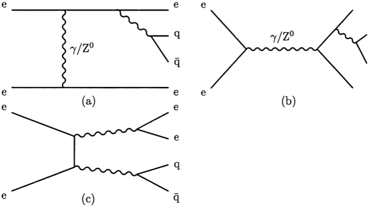
Much of the information on the hadronic structure of the photon has been obtained from measurements at e^e“ colliders, in interactions involving the photon ‘clouds’ th at surround the beam electrons. Of particular importance have been measurements of deep-inelastic electron-photon^ scattering. Fig ure 1.1, in which the structure of a nearly-real photon, 7, is probed by a highly virtual one, 7* of virtuality producing a hadronic final state, X. In this context, structure functions of the photon can be defined in analogy with those of the proton, although the point-like component leads to im portant differences in the behaviour of photon structure functions.
Measurements of the hadronic photon structure function such as th at described in this thesis, use the fact th at the differential cross-section of the process ey —^ eX as a function of and Bjorken x is proportional to Here and x can be thought of as the fraction of the photon’s momentum carried by the struck quark. Because the photon couples to electric charge, is in leading order proportional to the quark content of the photon.
Experimentally, F^ is measured using single-tagged events. is determined from the energy and polar angle of the deeply-inelastically scattered (tagged)
CHAPTER 1. INTRODUCTION
electron, which is generally well measured by the electromagnetic calorimetry of the detector. The electron which emits the quasi-real photon is scattered at a very low angle and escapes unobserved down, or close to, the beam pipe. As a consequence, the energy of the target particle is not known - in contrast to electron-proton DIS - and so x has to be determined by measuring the invariant mass of the hadronic final state. Because the e'y centre-of-mass system does not coincide with the laboratory frame, the hadrons tend to be boosted in the forward direction and thus poorly contained in the detector. For this reason a central component in measurements of F2 is the use of
an unfolding procedure to relate the visible x distribution to the underlying true distribution. As a result, the accuracy of photon structure function measurements does not approach those of the proton.
The measurement of the photon structure function now has a history going back some 20 years, when the first results were obtained with the PETR A collider a t DESY. Since then measurements have been carried out with P E P at SLAC, TRISTAN at KEK and, most recently, LEP at CERN. A summary of the world d a ta on F2 is shown in Figure 1.2, which is an updated version
of a figure taken from a recent comprehensive review [1]. The published measurements [2-18] range in from 0.24-390 GeV^, and down to ~ 10“ ^ in X . Several preliminary results from LEP experiments [19-21] are also
shown, including one from this analysis [21].
This thesis describes measurements of F2 made using d ata recorded by the
OPAL detector in the years 1997-2000 at e'^e" centre-of-mass energies of 183-209 GeV. It includes a high-Q^ measurement of as a function of
X (at an average (Q^), of 780 GeV^) and also the most precise OPAL
CHAPTER 1. INTRODUCTION
0.5
-z I I 1 1 1 i i i j I I 1 1 1 i r i | I I M i l l
o OPAL(1.9)
— GRV (HO)
T I ' I I I M l | I I I I I I I I ] I I I I I I L L
:: o O P A L ( 3 .7 )
fN
: (a) , □ L3(l,9) :: (b) , □ L3(5.0)
I . 11 iniil I I I I iiiil ] I I I III! I r I mill I I 11 iiiil
10-3 10 10
— GRV (HO)
r O 0.2
q
0
0.5
O 1*13 1 0 (2 .4 ) TI*(72y(2.83)
□ T OPAZ(5.1) A M l (6.8) OPA 179.9)
0.5
0
1
0.5
0
* T P (7 2y(9.24) □ T P (7 2y(9.38)
t i l l
A ALEPH(9.9) O PI3 1 0 (9 .2 )
OPA 1710.7)
: A AI.EPH(2(I.7) (I) - A DEI P ill |)il.( 19.0»
L3(23.1)
r S
A DELPHI pH.dOI.) I ( p ) O O P A 17135.)
* A M ’S (73.) ■ (c ■ JADEdOO.)
I ' □ T O P A 7 7 8 0 . ) T 0 L 3 ( i 2 0 . ) AaLEPH(284.)
“ I I I I I I I I r
* T PC /2y(0.71) - - X TP(72Y(1.31)
f i l l ---1
—t-0> P I3 1 0 (4 .3 ) * T PC /2y(5.1)
A DELPHI prl.(5.2) O OPA 178,9)
+ A DEI PHI(I2.(I)
A 1)1 EPHI prl.l 12.7)
+
O OPA 1717.5) ( k ) • OPA1717.8)
I . • OPA 1714.5) ■ L3(10.8) I > A L E P ll pM.(13.7) ■L3(15.35
A DELPHI p'il.(28.5) ( m )
A r \S S O (23.) ■ JA D E (24.)
A DELPHI p'rl.(40.) ( n ) » PELITO(45.) ^ ^
□ TOPA7716.) • OPA 1730.) AEEPH|prl.(?6.:>) A DELPHI pS 1.(700.) ( q ) ♦ AMV(390.)
O O P A L p r l.( 7 6 7 .)
J I I I I I I I L 0.5
Chapter 2
Theory of Photon Structure
2.1
T h e C ross-Section for P h o to n -P h o to n Scat
tering
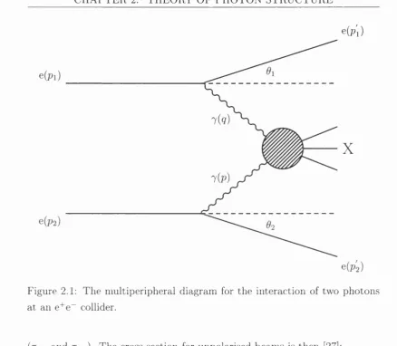
The m ultiperipheral diagram for the interaction of two photons of arbitrary virtuality at an e"^e“ collider is shown in Figure 2.1. The labels in brackets denote the four-vectors of the participants. The incoming electrons, of energy E'b, both radiate photons and are scattered at an angle 9i^2- The photons interact to produce a final state X, which in this thesis will always be regarded as hadronic, b ut could equally well be a lepton pair. (The leptonic structure of the photon has been measured by several experiments [14,22-26] and found to agree well with QED predictions.)
CHAPTER 2. THEORY OF PHOTON STRUCTURE
e(p'i)
Figure 2.1: The multiperipheral diagram for the interaction of two photons at an e"^e" collider.
(ttt and ttl)- The cross-section for unpolarised beams is then [27]: ,6 _ d^p'; d^p'2 f {q p f
-<7e.e--e+e-X g , 167r'>Q2p2 J
(4 /9 + +pJ + (Tt t + 2 | p + - p f - | T T T C O s 2 0 + 2 p + + p “ (TTL + 2p J" p J+ tT L T + 2 p “ p “ <^LL - 8 |p i^ “p 2 °k T L C O S (^ ) , ( 2 .1 )
where p'^ 2 are the momentum vectors of the scattered electrons and £[ 2
their energies, and ÿ is the angle between the scattering planes of the two electrons in the photon-photon centre-of-mass frame. The coefficients p“ 2i where a, 6 = T , —, 0 are the photon helicities, are elements of the photon
density m atrix and depend only on the kinematic variables and on ttIq. They are given in full in, for example. Equation 5.13 of reference [27].
________ CHAPTER 2. THEORY OF PHOTON STRUCTURE________
and the other is highly virtual (7*7 events). In this situation the expression for the cross-section simplifies considerably, since a real photon can have only transverse polarisation. The terms cttlj ctll and ttl vanish as —>■ 0. The term proportional to ttt also vanishes because for = 0 the angle ÿ is undefined. Thus Equation 2.1 reduces to
16 ^ d^p; d^p^2 ( {q-pY - \
E[ E'2 167r4Q2p2 ^ (pi . p2)2 - /
4/9++P++ I (Ttt + • (2.2) Only the term s c ttt and a i r remain, corresponding to the probing of a transverse target photon by, respectively, a transverse or longitudinal virtual photon.
2.2
T he Equivalent P h o to n A pproxim ation
It is usual to factorise the cross-section of Equation 2.2 into two terms: an expression for the flux of incoming, transversely polarised, quasi-real target photons, and a term describing the reaction 07 eX. This can be written as
dVe+e--.e+e-X = ( / P^) d P ^ ) • , (2.3) which is derived from Equation 2.2 in Reference [1]. The integral term is the Weizsacker-Williams [28] formula for the flux of real photons. The flux factor
CHAPTER 2. THEORY OF PHOTON STRUCTURE
acceptance, leading to
/
'■«■O'’ - S1 + (1 z f _ 2m !z ( ^
p 2 I p 2 p 2
m z n \ m i n m a x
(2.5)
2.3
P h o to n Structure Fuuctious
It is normal to describe the cross-section for 07 eX (the second term in Equation 2.3) in terms of structure functions of the real photon. It is useful, therefore, to define the usual DIS invariant variables which, neglecting the electron mass, are:
= —q^ = 2 Eb Etag (1 — cos ^tag) 5 (2.6)
^
2 q - p + + ^ >
y = = (2.8)
Pi ' P 2
where the experimentally measurable variables Eta.g and ôt&g are the energy and polar angle respectively of the tagged electron, and W is the invariant mass of the hadronic final state, X. In the DIS limit f ^ % 0, and so
is neglected in the calculation of x from Equation 2.7.
The transverse and longitudinal structure functions of the photon are defined, in the limit P^ = 0, as [31]:
47T^a Through use of the above and the relation
PZ = 7% -(7L T . (2.10)
________ CHAPTER 2. THEORY OF PHOTON STRUCTURE________
The experimental requirement of a high tag energy means th a t only low val ues of y are studied, rendering negligible the term proportional to F^. Thus the structure function F2 can be related through a simple proportionality
factor to the differential cross-section for 67 scattering.
7
2.4
T heoretical P redictions for
F2
The hadronic structure of the photon can be viewed, in analogy to the proton, in terms of a sum of distributions of partons in the photon. In this view, and in leading order.
F2^(o;,Q2) = -Hç7(o:,Q2)] , (2.13) i=l
where q] is the parton distribution function parameterising the probability of finding a quark, of flavour i and charge e*, within the photon at a given
As mentioned in the introduction, can be regarded as the sum of two parts - the point-like and the hadron-like components. The point-like part is most im portant at higher x and and is most simply approximated by the quark-parton model, whilst the description of the hadron-like part, which dominates at low x and is usually based on a vector meson dominance ansatz. These models are described in the two sections which follow.
2.4.1 Quark Parton Model
CHAPTER 2. THEORY OF PHOTON STRUCTURE
7 q
Figure 2.2: The box diagram for the process 7*7 —^ qq.
of F2 is based on the box diagram for the process 7*7 —» qq shown in
Figure 2.2 which, for the real photon, leads to [32]
^ Q P M = ^ + ( 1 - In ( ^ ^ 2 ™ + 8 a : ( l - x ) - 1
^ i=l L \ ''^i /
(2.14)
where the sum runs over all active flavours (4m? < where rrii is the quark mass).
CHAPTER 2. THEORY OF PHOTON STRUCTURE
1.4
QPM, Q =780 GeV"
QPM, Q^=12.1 GeV
1.2Simple VMD
TPC/2y VMD
10.8
0.6
0.4
0.2
0.9
0
0 0.1 0.2 0.3 0.4 0.5 0.6 0.7 0.8 1
________ CHAPTER 2. THEORY OF PHOTON STRUCTURE________
2.4.2 Vector Meson Dominance
The hadron-like p art of the photon cannot be calculated by current theoreti cal techniques, since the problem is non-perturbative in nature. Because the photon couples to the = 1 vector meson states (e.g. p, w, 0), the usual way of estim ating the hadron-like part is to use a vector meson dominance (VMD) model. The parton distributions of the vector mesons have not been measured, b ut the structure function of the p can be approximated by th a t of the pion, which is known experimentally [33]. Using this basis, estimates for the VMD component can be arrived at via various assumptions. As an example, the simplest VMD estimate is obtained by taking contributions of
p and w, leading to [31, 34]
^VMD = 0 . 2 a ( l - T ) , (2.15) which applies to ~ 10 GeV^.
An alternative approach is to parameterise a VMD component by fitting to measurements of the pion structure function, or to low-Q^ F<7 data. The latter has been done by the T P C/ 2 7 Collaboration [6], and their fit, which was to d a ta at (Q^) = 0.7 GeV^, gives
P2.VMD = « (0.2 2x®-^'(l - + 0.06 (1 - . (2.16)
Caution should be accorded to this fit, though, since the highest x point used corresponds to very low W - deep into the poorly understood region of resonance production.
________ CHAPTER 2. THEORY OF PHOTON STRUCTURE________
2.4.3
QCD and the Evolution of
F
2with
Although the size and shape of F2 at a given, finite cannot be calculated
because of the hadron-like part, the evolution of with can be deter mined within the framework of perturbative QCD. It should first be noted, however, th a t even the naive parton model predicts a logarithmic increase of
F2 with (Equation 2.14) - unlike which exhibits Bjorken scaling in this
model, which is only broken once QCD corrections are taken into account. This feature of F j arises because of the point-like part of the photon, which leads to positive scaling violations at all values of x (Figure 2.4). Contrast this with the case of the proton (Figure 2.5), where gluon radiation leads to negative scaling violations at large x and pair production of quarks from gluons results in positive scaling violations at small x.
The original QCD evaluation of F2 was undertaken by W itten using the
technique of operator product expansion [35]. He found th a t both the shape and normalisation of F^ s^re calculable at asymptotically large and th a t the evolution of F ^ is similar to the QPM case:
(2.17) at leading logarithmic order. The asymptotic solution has been re-derived using Feynman diagrams [36, 37], evolution equations [38] and in NLO [39]. In addition, param eterisations based on this method have been presented [40- 42].
CHAPTER 2. THEORY OF PHOTON
s t r u c t u r e
Î
1
4 i w ^. ! . « S ' i p r t ) ' ' * ' ' ® " ' r l ’c ' ' ^ : ; : ^ h<v < * >
’ - '
'1
4 k ■^ 0.70 - - - ^ ~ - i ^ ■"? i
3 k'" f ; : : ^ : F
^ 0.J5 - ;--- 7 -|~ ~ ~ jf ~ . ~ ~ f ~ ~ ^ 7-;^-7.-r j- -^
^ ^*-25 fff ~ | — ji:.jr.
-j 1 - â - irrr : { : : : : :
- --»-- «b?T ^ ,^=.^._..^.
1 0-' ,
^ 1 0^
'' « « '• ' ' ‘ ' " • ' ' “I
from Reference fij, «^-^ren.ents of the evolution of Taken
CHAPTER 2. THEORY OF PHOTON STRUCTURE
ZEUS+Hl
ZEUS 96/97
OX 4
HI 96/97 ☆ HI 94/00 Prel. A NMC, BCDMS, E665
ZEUS NLO QCD Fit (p r e l. 2 0 0 1 ) HI NLO QCD Fit
3.5
x = 0 . 0 0 8
x = 0 . 0 1 3
x = 0 . 0 2 1
2.5
x = 0 . 0 3 2
x = 0 . 0 5
-É - a y g -A- t ^ '4 4 "a
1.5
x - 0 . 1 3 x=0. 1
= 0 .2 5
x = 0. 4
0.5
x = 0 . 6 5
________ CHAPTER 2. THEORY OF PHOTON STRUCTURE________
radiated gluons can in tu rn produce sea quarks with even lower momentum. Thus, for the hadron-like part of the photon, a shift from high to low x is expected with increasing In addition, the point-like p art increases with
for all X .
In order to calculate F2 at a given scale, one needs to first fix the input x
distribution at some low scale, based either on theoretical considerations or a fit to F2 data. Then the evolution of the quark and gluon distributions is
given by the DGLAP [44] equations, which to leading order are:
(2.18)
àgi(x,Q'^) _ d log Q2 27T
These equations apply to massless quarks. The Pij{z) are splitting functions which express the probability of finding a parton of type i within a parton of type j with momentum fraction 2. For a good discussion of the evolution equations as applied to the photon see Reference [45], which also covers the extension to NLO.
The evolution of remains logarithmic, the running of balancing the effects of gluon emission. If as were fixed, F7 would bend with to become asymptotically scale-invariant at large [34]. A measurement of the evolution, using as long as possible a lever arm in is therefore a good test of perturbative QCD predictions. It also holds out the possibility of obtaining a competitive measurement of ag [46].
2.5
H eavy Quarks
________ CHAPTER 2. THEORY OF PHOTON STRUCTURE________
can only be regarded as massless at high scales and large invariant masses. Massive quark DGLAP equations have been derived [47], but the treatm ent can be simplified by the hard scale resulting from the mass. This means th a t the zeroth-order QCD calculation (i.e. QPM, but not neglecting the mass terms), known as the Bethe-Heitler formula, is a good approximation and in particular deals with the threshold ( W = 2mc) behaviour correctly [48]. This is in contrast to the QPM (see Figure 2.3); in reality the cut-off should not be sharp because the phase space for charm production is limited near the threshold.
The charm contribution is expected to be almost entirely point-like in the x
region considered in this thesis, but at low x a LO resolved contribution does come from photon-gluon fusion. The charm structure function 7^^ has been calculated to NLO [49], and has recently been measured by OPAL [50]. The production of b quarks is suppressed by the larger mass and small charge, and is negligible at LEP2 energies.
7
2.6
T he
P
D ep en dence o f
F
2In the discussion above the target photon has been assumed to be real, i.e. = 0. In fact, because of the incomplete experimental acceptance in the very forward direction, is only restricted to be less th an a fixed maximum. The effect of this is twofold; first, the flux of target photons is affected, and second, the structure function P^(x, Q^, P^ ^ 0) is in general not expected to be equal to P^(rc, P^ = 0).
CHAPTER 2. THEORY OF PHOTON STRUCTURE
c/5
3
O C /5 "C
3
1
0.8
0.6
X = 0.9
0.4
X = 0.5
SaSlI) (IF2=0)
: SaSll)(IP2=2)
: - - ( ;k s : Q^ = 30GeV^
0.2
X = 0.1
3
0 0.5 1.5 2 2.5
P“ [GeV^
________ CHAPTER 2. THEORY OF PHOTON STRUCTURE________
calculated at LO and NLO [51] in the limit ^ » A^. The hadron-like part is expected to be suppressed as increases, but the rate of the fall- off is theoretically uncertain and the experimental knowledge is very poor. PLUTO [52] and L3 [17] have measured the virtual photon structure function (= F-7 + 3 7 ^ /2 ), but with severely limited statistics, and d a ta have also been presented by the HERA experiments [53]. D ata do not exist on the structure functions of virtual mesons, making the choice of a suitable VMD input to the parameterisations a difficult one. The outcome of all this is th a t the different parameterisations of the dependence of P^ show large discrepancies, as dem onstrated in Figure 2.6, although the qualitative behaviour is the same.
7
2.7
P aram eterisations o f
F
2A number of parameterisations of the real photon structure function have been presented, in both leading and next-to-leading order, based on the DGLAP evolution equations. The various sets differ in the chosen starting scale for the evolution, in the input distributions assumed at th a t scale and in the amount of d ata used to determine any free parameters. There are also choices to be made with respect to the value of the QCD scale A, the treatm ent of charm and, for the NLO sets, the factorisation scheme.
The choice of the input quark and gluon distributions can be based either on theoretical prejudice (usually some VMD-based argument), on a phenomeno logical fit to the data, or on a combination of the two. The quark distribution is by now reasonably well constrained by the data, at least in the central x
________ CHAPTER 2. THEORY OF PHOTON STRUCTURE________
low a; - a region where measurements have only recently become available - and even there only indirectly. D ata exist which are directly sensitive to the gluon distribution of the photon, such as jet production d ata from LEP and HERA, but no significant effort has yet been made to incorporate these results into any parameterisation.
2.7.1
Gluck, Reya and Vogt (CRY)
The GRV param eterisation [56] is available in LO and NLO, and was moti vated by the successful description of the proton and pion structure functions by the same authors. The evolution is started from a very low scale (0.25 GeV^ for LO and 0.3 GeV^ for NLO) and the input distribution is a purely hadron-like one based on VMD arguments. The point-like part is generated dynamically with the evolution equations. The VMD input is the same for both the quark and gluon distributions and takes the form x/tt ~ x“ (1 — x)^, where a and b are obtained from measurements of the pion structure function. The only free param eter is the normalisation of the VMD input, correspond ing to the uncertainty in the inclusion of the uj and 0 mesons. It is determined by fitting to d ata in the region 0.71 < < 100 GeV^, and W > 2 GeV to avoid the resonance region. Charm and bottom quarks are included via the Bethe-Heitler formula, with rric = 1.5 GeV and mi, = 4.5 GeV, and are treated as massless in the evolution at high values of W . These param eteri sations are by now somewhat elderly, yet in general they still do a good job of describing all the current F2 data.
2.7.2
Gluck, Reya and Schienbein (GRSc)
________ CHAPTER 2. THEORY OF PHOTON STRUCTURE________
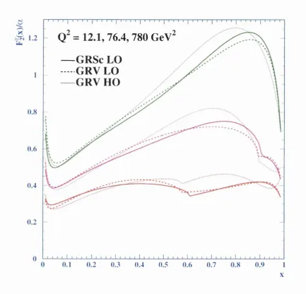
of the incoherent sum of the GRV parameterisation. This eliminates the only free param eter and means th a t no fit to d ata was required. The charm contribution was added using the Bethe-Heitler formula, but the charm mass used was reduced to 1.4 GeV. The GRSc LO param eterisation is compared to the LO and NLO GRV curves, at three values of in Figure 2.7. Note th a t, particularly at low Q^, the differences between the GRV LO and NLO param eterisations are greater than those between the two LO sets.
2.7.3 Hagiwara
et al
(WHIT)
The W HIT LO parameterisations [48] start their evolution at a relatively high starting scale of 4 GeV^. This means th a t the input distributions need to include some point-like contribution, and the input valence quark distribution is parameterised by xq {x )/ a = A x ^ { l — x)^, with the coefficients obtained from fits to d a ta in the range 4 < < 100 GeV^. The sea quark distribution is approximated by the Bethe-Heitler formula using r r i q = 0.5 GeV. Charm
is included via Bethe-Heitler for < 100 GeV^ and through the use of the massive evolution equations for higher values of Q^. The charm mass is taken to be 1.5 GeV. The gluon input distributions take the same functional form as the valence quark input, but the coefficients are systematically varied within the limits allowed to still be consistent with the data. This results in six different sets of parton distribution functions. However, because the gluon distribution only has a strong effect at low x, the differences between the sets are small for the values of a; (a; > 0.1) considered in this thesis.
2.7.4
Schuler and Sjostrand (SaS)
CHAPTER 2. THEORY OF PHOTON STRUCTURE
Q" = 12.1, 76.4, 780 GeV
1.2— GRSc LO
GRV LO
GRV HO
10.8
0.6
0.4
0.2
0.1 0.2 0.3 0.4 0.5 0.6 0.7 0.8 0.9 1
Figure 2.7: The GRV LO and HO and GRSc LO parameterisations of shown at three values of for which results are obtained in this thesis. The kink in the curves at the two lower values of are due to the charm threshold, which sits at an x value determined by the charm mass used and
________ CHAPTER 2. THEORY OF PHOTON STRUCTURE________
factorisation schemes, leading to four sets in all. For the SaS2 sets the shape and normalisation of the hadron-like input distribution is determined by fitting to F2 data. For the SaSl sets only the shape is obtained from a fit to F2 data, whilst the normalisation is taken from an analysis of 7p data. Bethe-
Heitler contributions of charm and bottom are included, with me = 1.3 GeV and mb = 4.6 GeV.
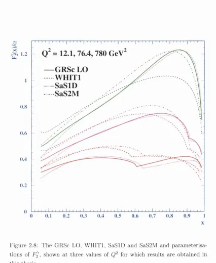
Two of the SaS sets, ID and 2M, are compared to the W H IT l and GRSc LO param eterisations in Figure 2.8. It can be seen th a t the GRSc LO and SaS ID curves are very close to one another, particularly at high The SaS sets are quite different from one another, especially at low Q^. The W H ITl curves show their strongest difference to the others at high x and
2.7.5
Other Parameterisations
CHAPTER 2. THEORY OF PHOTON STRUCTURE
Q" = 12.1, 76.4, 780 GeV
1.2— GRSc LO
W HITl
SaSlD
SaS2M
1
0.8
0.6
0.4
0.2
0
0.9
0 0.1 0.2 0.3 0.4 0.5 0.6 0.7 0.8 1
Chapter 3
LEP and the OPAL Detector
3.1
LEP
The LEP collider at CERN, an e‘*"e“ collider of 27 km circumference, op erated between the years 1989 and 2000. During the first phase (L E Pl, 1989-1995) the beams were accelerated using room tem perature copper cav ities and collided at centre-of-mass energies, y/s, close to the mass of the
TP. For the second phase of LE P’s life (LEP2, 1995-2000) superconducting rf accelerating cavities were added, bringing ^/s past the threshold for the production of W'*'W~ pairs and ultimately up to ~209 GeV in the pursuit of new physics.
CHAPTER 3. LEP AND THE OPAL DETECTOR
CERN Accelerators
A L E PH
O P A L
D ELPHI
West Area
bast Area
ele c tro n s p o s itro n s pro to n s a n tip ro to n s P b ions
T T L 2
L E A R
South Area
P P b i o n s
LEP; Large Electron Positron collider SPS: Super Proton Synchrotron AAC: Antiproton Accumulator Complex ISOLDE: Isotope Separator OnLine DEvice PSB: Proton Synchrotron Booster PS: Proton Synchrotron
LPl: Lep Pre-Injector
EPA: Electron Positron Accumulator LIL: Lep injector Linac
LINAC: LI Near Accelerator LEAR: Low Energy Antiproton Ring
R u d o lf LEY , PS D iv is io n , C E R N , 0 2 .0 9 .9 6
_________ CHAPTER 3. LEP AND THE OPAL DETECTOR_________
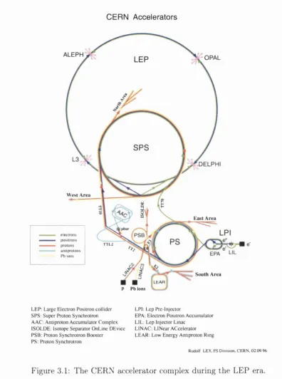
LEP was the last accelerator in a chain of five, which are illustrated in Fig ure 3.1. The injectors consisted of two linacs of 200 and 600 MeV, fed by an electron gun and a positron converter, followed by the 600 MeV Electron- Positron Accumulator, which injected into the CERN PS operating as a 3.5 GeV e+e~ sychrotron. The electron and positron bunches would then pass from the PS into the SPS, which accelerated them to 22 GeV prior to their injection into LEP.
3.2
T h e OPAL D etector
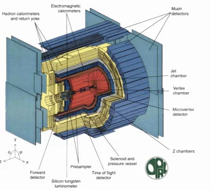
OPAL [62] was one of the four large detectors situated around LEP. It was a multipurpose apparatus designed to efficiently detect all types of interactions occurring in e"^e" collisions, with nearly full solid angle acceptance. The detector was made up of a number of subdetector systems, the information from which was combined to reconstruct the events.
CHAPTER 3. LEP AND THE OPAL DETECTOR
Hadron calorim eters and return yoke
Electromagnetic calorimeters
Solenoid and pressure v e sse l Presampler
Time of flight detector Forward
detector
Muon detectors
Jet cham ber
Vertex cham ber
Microvertex detector
Z cham bers
Silicon tungsten luminometer
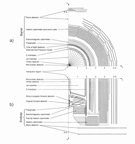
CHAPTER 3. LEP AND THE OPAL DETECTOR
a)
b)
(0
CO
Q .
I
C
LU
^ M uon d e te c to r
H a d ro n c a lo r im e te r a n d re tu rn y o k e *
E le c tr o m a g n e tic c a lo r im e te r - P r e s a m p i e r
----^ T im e o f flight d e te c to r ---S o le n o id a n d P r e s s u r e V e s s e l
Z c h a m b e r s J e t c h a m b e r ---V e rte x d e t e c t o r ---M ic ro v e rte x d e te c to r
5 m In te ra c tio n reg io n
5 m M ic ro v e rte x d e te c to r
V e rte x d e te c to r ---J e t c h a m b e r
Z c h a m b e r s
S ilic o n -tu n g s te n fo rw a rd d e te c to r
O rig in al fo rw a rd d e te c to r
^ P r e s a m p le r
E le c tr o m a g n e tic c a lo rim e te r
P o le tip h a d ro n c a lo r im e te r ■
H a d ro n c a l o r i m e t e r ---M uon d e te c t o r
4
6 m
_________ CHAPTER 3. LEP AND THE OPAL DETECTOR_________
The critical subdetectors to the present analysis are, firstly, those used to tag the scattered electrons from two-photon collisions and, secondly, those im portant to a good reconstruction of the invariant mass of the hadronic final state. In this analysis, electrons are tagged in the endcap electromag netic calorimeters and the forward detectors. A good understanding of the response of these detectors to high energy electrons is vital, and significant work has been invested to achieve this (see in particular Appendix A). For reconstructing the hadronic part of the event (which is mostly low energy) we rely most heavily on the jet chamber and the electromagnetic calorimetry. In the OPAL coordinate system the z-direction points in the direction of the electron beam (which was anti-clockwise when viewing LEP from above). The a;-axis is horizontal and points towards the centre of LEP. The z-axis is inclined at an angle of 13.9 mrad with respect to the horizontal plane; thus the y-Qxis is inclined by the same amount with respect to the vertical. The polar angle, 6, is measured from the z-axis, and the azimuthal angle, <^, from the a:-axis about the z-axis.
3.2.1
Central Tracking System (CT)
S ilicon M icro v ertex D e te c to r (SI)
_________ CHAPTER 3. LEP AND THE OPAL DETECTOR_________
V ertex D e te c to r (C V )
The vertex detector was a i m long, 470 mm diameter, cylindrical drift chamber th a t was located between the outer (original) beam pipe and the jet chamber. It operated within the common 4 bar central tracking system pressure vessel and contained a mixture of argon, m ethane and isobutane. An original component of OPAL, it was used to determine the positions of decay vertices of short lived particles and to improve the overall momentum resolution of the central tracking system. It was segmented radially, and had an inner layer of 36 cells with axial wires and an outer layer of 36 stereo cells with wires strung at an angle of 4°. The axial cells provided a measurement of points in the r — (f) plane with a resolution of 50 //m. The combination of the stereo and axial cell information allowed a resolution of 700 /im on the ^-coordinate of charged particles close to the interaction region.
J et C ham ber (C J)
The central jet chamber was a large volume gaseous detector. It recorded the tracks of charged particles and determined their momenta by measuring their curvature in the magnetic field. Particle species identification was provided by measuring the rate of energy deposition, d E / d x , of particles traversing the chamber. The sensitive volume of the jet chamber was a cylinder of length approximately 4 m, surrounding the beam pipe and vertex detector. The inner diameter was 0.5 m, the outer 3.7 m. The chamber was divided in (f)
_________ CHAPTER 3. LEP AND THE OPAL DETECTOR_________
electrons were measured in this analysis.
Z C ham bers (CZ)
The Z chambers were arranged to form a barrel layer around CJ, covering the polar angle range 44° < 9 < 136°. They improved the polar angle resolution, and hence the invariant mass determination, by making a precise measurement of the z coordinate of charged particles exiting CJ. CZ was made up of 24 chambers, each 4 m long, 50 cm wide and 59 mm thick. The chambers were divided into eight cells in z. Each cell was 50 cm long with six readout wires strung along the <j) direction. The resolution in z was 100-350 jim .
3.2.2
Timing Counters
The time of flight barrel system (TB) generated trigger signals and allowed charged particle identification in the range 0.6-2.5 GeV by measuring the transit time from the interaction point. It also aided in the rejection of cos mic rays. It consisted of 160 scintillation counters and covered the region I cos 9 I < 0.82, forming a barrel of mean radius 2.36 m outside the solenoid. In addition to this barrel section, a scintillating tile system [64] was installed in the endcap region in 1996. Called the Tile Endcap (TE) system, it pro vided timing information - allowing the identification of which bunch of a train an event belonged to - and the ability to detect minimum ionising particles.
3.2.3 Electromagnetic Calorimeter
_________ CHAPTER 3. LEP AND THE OPAL DETECTOR_________
to beam energy. It was a total absorption calorimeter consisting of three large arrays of lead glass blocks, covering 98% of the solid angle. Since there was about 2 Xq of m aterial in front of the lead glass, mostly due to the coil and pressure vessel, most electromagnetic showers were initiated before the lead glass itself. Presampling devices were installed in both the barrel and endcap regions, to measure the position and sample the energy of these showers, thereby improving the electromagnetic energy resolution.
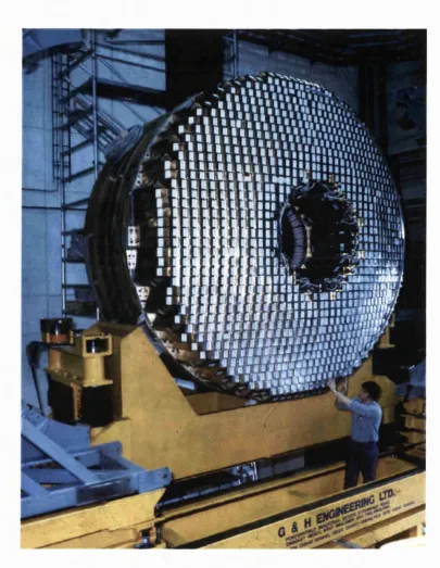
E ndcap L ead-G lass C alorim eter (EE)
The endcap electromagnetic calorimeters [65], one of which is pictured in Figure 3.4, were used to tag the electron in two-photon collisions in this analysis. Each endcap was composed of 1,132 lead glass blocks assembled in a dome-shaped array and located between the pressure bell of the central tracking system and the pole tip hadron calorimeter. The detector covered the full azim uthal angle and 0.81 < | cos 6 | < 0.98 (200-630 mrad). Because of space constraints, the lead glass blocks were mounted coaxially with the beam line.
The 9.2 X 9.2 cm^ blocks were manufactured in three lengths (38, 42 and
52 cm) and arranged, following the contours of the pressure bell, so th a t they presented a to tal depth of at least 20.5 radiation lengths, and more typically 22 Xq, to all particles coming from the interaction region. The blocks were instrum ented with single stage multipliers known as vacuum photo triodes (V P T ’s), which were developed to be able to operate in the full magnetic field.
The performance of the calorimeter was extensively studied, prior to installa tion, in 7r“ and e~ beams. The energy response was found to be linear in the range 3-50 GeV and the energy resolution was œe/ E ^ 5 % /\/Ë (where E
CHAPTER 3. LEP AND THE OPAL DETECTOR
_________ CHAPTER 3. LEP AND THE OPAL DETECTOR_________
separate reference light sources were incorporated into the assemblies. These corresponded to ~ 10 and ~20 GeV electron equivalents, and were used to monitor the performance of the detector throughout its lifetime.
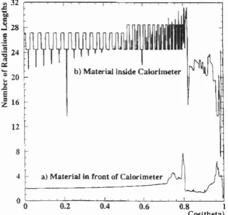
It is im portant to note th a t the resolutions quoted above correspond to the in trinsic resolution of the calorimeter, and not the resolution actually observed once the detector was in situ. This was degraded due to a combination of the m aterial in front of the calorimeter and the severe space constraints in the endcap region, which in some areas led to reduced active m aterial being presented to particles coming from the interaction point. Figure 3.5 shows the number of radiation lengths of material in front of and inside the entire electromagnetic calorimeter. The right hand part of the figure pertains to the EE.
B arrel L ead-G lass C alorim eter (E B )
The barrel calorimeter consisted of a cylindrical array of 9,440 lead-glass blocks of 24.6 Aq, located at a radius of 2.455 m, covering the full azimuthal angle and | cos 6 | < 0.98. In contrast to the endcaps, the blocks were ar ranged so th a t they pointed close to the nominal interaction point (but not exactly at it, in order to prevent the escape of neutral particles through the gaps between blocks). Each block was ~10 x ~10 cm^ in cross-section and 37 cm in depth. The blocks were instrumented with magnetic field tolerant phototubes. The energy resolution of a prototype barrel section was mea sured, in a testbeam , i o h e ge/ E — 0.2% -f 6.3%/y / Ë (E in GeV) with no m aterial in front of the calorimeter.
P resam p ler
CHAPTER 3. LE? AND THE OPAL DETECTOR
U 28
b) Material Inside Calorimeter
“ 20 r
a) Material In front of Calorimeter
0.8 1
Cos(theta)
Figure 3.5: “Radiation lengths (a) in front of and (b) inside the active ma terial of the electromagnetic calorimeter as a function of | cos 9 | at an ar bitrary angle in 0. The peaks in the material in front of the calorimeter at I cos 9 I ~ 0.8 and ~ 0.96 arise from the structure of the pressure bell of the central tracking system. The structure in the active m aterial of the calorimeter arises, for | cos ^ | < 0.8 from the quasi-pointing block geome try, at I cos 9 I = 0.8 from the barrel/endcap overlap and transition, and at
_________ CHAPTER 3. LEP AND THE OPAL DETECTOR_________
of gaseous wire chambers working in limited streamer mode. In the endcap region the presampler was an umbrella shaped arrangement of thin gaseous multiwire chambers which were operated in a high gain mode. Combining the information from the presampler with th a t from the calorimeter provides an improved energy resolution on a shower by shower basis, because the number of charged particles passing through the presampler is approximately proportional to the energy deposited in the m aterial traversed before the presampler. However, because of reliability issues, the presamplers were not used in this analysis.
3.2.4 Hadronic Calorimeter
The hadron calorimeter (HCAL) measured the energy of hadrons th a t pen etrated the electromagnetic calorimeter. The iron of the return yoke was segmented into layers, with planes of wire chambers between each layer, and formed a cylidrical sampling calorimeter about 1 m thick. To achieve good coverage in solid angle, the detector was constructed in three parts - the bar rel, the endcaps and the pole tips - presenting at least 4 interaction lengths of absorber over 97% of 47t. Most hadronic showers were initiated in the 2.2
interaction lengths of m aterial in front of the hadronic calorimeter, so the overall hadronic energy was determined by combining information from both the electromagnetic and hadron calorimeters.
3.2.5 Muon Chambers
_________ CHAPTER 3. LEP AND THE OPAL DETECTOR_________
penetrated to the muon detector and left a single clean track, the probability of a pion not interacting, thus faking a muon, was less th an 0.001. The muon chambers are not used in this analysis.
3.2.6 Forward Region
Detectors in the forward region extended the electromagnetic calorimetric coverage of OPAL to low angles with respect to the beam line. They are used in this analysis to tag scattered electrons from two-photon collisions, but their main purpose was to provide precision measurements of the luminosity delivered to OPAL by counting small-angle Bhabha scattering events. Of relevance to this analysis is the fact th a t hadronic showers were not well contained by these electromagnetic calorimeters, resulting in poor hadronic energy measurement in the forward region. A diagram of the layout of the forward region is shown in Figure 3.6.
Forward D e te c to r (F D )
The FD consisted of four separate parts: the main calorimeter, the tube chambers, the gamma catcher and the far forward monitor. Two further original components, the drift chambers and the fine luminosity monitor, were removed to make room for the silicon tungsten calorimeter (see below) and will not be discussed further. The two FD assemblies, one situated at each end of the OPAL detector, were symmetric about the interaction point. The forward calorimeter consisted of 35 layers of lead-scintillator sandwich, presenting a to tal of 24 X q to electrons coming from the interaction point.
CHAPTER 3. LEP AND THE OPAL DETECTOR
iff
Ü313WIW01V3 0NV1AÜVM
SW3ÜNVH3 3ani
I
il
o
nqoz - /_________ CHAPTER 3. LEP AND THE OPAL DETECTOR_________
was ±1.5°. The energy resolution was measured to be g e/ E ~
[E in GeV) and the radial position resolution on electron showers, using the ratio of the inner to outer signals, was ± 2 mm. There was clean acceptance for particles from the interaction region for 60 < ^ < 120 mrad. The tube chambers, located between the presampler and the rest of the main calorime ter, consisted of three planes of proportional tubes, with two layers aligned at right angles and the third at 45° to the other two. They improved the position resolution to about 2 mrad in both 6 and (}>.
The gamma catcher, a non-containing lead-scintillator ring of 7 Xq, filled the gap between the EE and the main FD calorimeter. The far forward monitors were two small lead-scintillator calorimeters mounted on either side of the beam pipe at ±7.85 m from the interaction point. They were used to provide a high statistics online luminosity measurement, and also to tag very low- angle (5 < ^ < 10 mrad) electrons. Neither of these last two components were used in this analysis.
S ilicon T u n g sten C alorim eter (SW )
_________ CHAPTER 3. LEP AND THE OPAL DETECTOR_________
3.2.7 The Trigger
The OPAL trigger system [67] was designed to reduce the 45 kHz LEP bunch crossing frequency to a manageable rate of ~ 10 Hz, by making a rapid deci sion on whether a bunch crossing might contain an interesting physics event. It was also used to reject backgrounds arising from cosmic rays, beam-gas interactions and subdetector electronics noise. Most physics events would be triggered by a number of independent conditions imposed on the subdetec tor signals. Such redundancy leads to a high trigger efficiency and is greatly beneficial to the estim ation of this efficiency.
The various trigger signals were combined in a flexible manner in the central trigger logic. The 47t solid angle of the detector was divided into 144 overlap ping bins, 6 in ^ and 24 in (/>. Events were triggered by certain programmable coincidences in the same 6-(f) bin. In addition, the subdetectors delivered stand-alone signals, based on total energy or track multiplicity sums, which could also trigger the readout of the detector. The trigger signals im portant to this analysis are listed in Table 3.1. A trigger decision would be reached approximately 15 ^s after the bunch crossing, and it took about 4.5 /is to reset the subdetectors, if appropriate.
3.2.8
D ata Acquisition
CHAPTER 3. LEP AND THE OPAL DETECTOR
Trigger name Subdetector Description
SWHIOR SW Total energy at either end > 34 GeV FDHIOR* FD Total energy at either end > 35 GeV
EEL(R)HP EE EM energy in left (right) endcap > 2 .4 GeV EEL(R)LO EE EM energy in left (right) endcap > 1.6 GeV TPEM L(R) EE Energy in 1 0 bin > 0 .7 5 GeV
EBTOTLO EB Total EM energy in barrel > 1 .8 GeV EBWEDGE EB Energy in ‘wedge’ > 2 GeV
E B l EB > 1 </) bin
TBM1(2,3*) CT > 1 (2,3) barrel tracks T PTTR (L) CT > 1 (/) bin in 6\ {6q)
T P T T l CT > 1 6-(j) bin
T P T T T O B C T /T B > 1 9-(f) coincidence in barrel TPTTEM* CT/ECA L > 16-(t) coincidence
TPTO B TB > 1 0 bin
TPTO EM B T B /E B > 16-(j) coincidence TBEBS T B /E B Same 0 sectors hit
Chapter 4
Monte Carlo Simulation
Monte Carlo programs are a crucial part of the analysis presented here. Not only are they used to refine the event selection, to determine the selection efficiency for signal events and to estimate physics backgrounds, but they are also required as an input to the unfolding procedure, to determine the correlation between the measured and true x distributions (see Section 7.1). It is therefore im portant to have Monte Carlo models which give a good description of 7*7 events, and in particular of the angular distribution of hadrons in the final state. This is not a trivial ambition, since we are dealing with non-perturbative QCD and multi-particle final states, meaning th a t any model has to use a series of approximations and assumptions.
CHAPTER 4. MONTE CARLO SIMULATION
4.1
HERW IG
HERWIG is a general purpose QCD Monte Carlo generator which includes electron-photon DIS. Its general philosophy is to provide the most complete treatm ent possible of perturbative QCD, combined with a simple model for soft interactions. It does this uniformly for any combination of lepton, hadron or photon scattering, allowing the free param eters to be tuned to one reac tion, for example e'*'e“ annihilation or pp scattering, and then applied to other reactions. This is a strong advantage, which lends confidence to the description of the underlying physics, since in a dedicated two-photon gen erator (as used in all measurements of until relatively recently) one can only tune the parameters to the very thing one is trying to measure, possibly biasing the measurement. HERWIG bases the event generation on the fact th a t an event can be factorised into several separate stages. These are:
• the production of a quasi-real photon from one of the beam electrons, • the elementary hard sub-process,
• initial and final state QCD radiation (parton showers), • the hadronisation process.
CHAPTER 4. MONTE CARLO SIMULATION
The participant quark in the hard scattering may emit QCD radiation before or after the scatter, with the probabilities of such emissions governed by the DGLAP splitting functions. The accurate treatm ent of the perturbative phase of these parton showers is one of the main emphases of HERWIG. For both the initial and final state parton showers (ISPS and FSPS), the evolution is calculated downwards in scale, away from the hard scatter, using the transverse momentum as the evolution param eter and obeying angular ordering. This means th at the ISPS uses a ‘backward evolution’ algorithm, back towards the incoming photon. The ISPS is analogous to the case of ep DIS - using NLO m atrix elements for the processes q qg and g qq
- with the addition of the 7 —^ çg vertex. The evolution continues by the emission of partons at successively lower angles, either until the quark is evolved back to the incoming photon, or until the cut-off scale is reached. In the former case the event is classified as point-like, otherwise it is hadron like (note th a t this separation is different to the choice made in the parton distribution functions). The photon rem nant will have a larger transverse momentum for point-like events, as given by perturbative QCD; for hadron like events the remnant is given a transverse momentum kt with respect to the direction of the incoming photon. The backward evolution algorithm ensures th at, at each branching, the parton distributions agree with the input parton distribution functions. All partons produced in the ISPS undergo further showering just like any other outgoing parton.
CHAPTER 4. MONTE CARLO SIMULATION
case these clusters then decay isotropically in their rest frame into pairs of hadrons, with branching ratios determined by density of states. If a cluster is too light to decay into two hadrons, it is converted to the lightest single hadron of its flavour, with the extra four-momentum donated to a neigh bouring cluster. A small fraction of clusters may be too heavy for two-body decay to be a reasonable ansatz; these are fragmented collinearly into two lighter clusters.
4.1.1 The A;t(dyn) modification
The default version of HERWIG 5.9 was found [72] to exhibit a less point like behaviour th an the d a ta in certain variables relating to the hadronic final state. In a first attem p t to improve the description of the data, the distribution of transverse momenta, kt, of the photon rem nant in hadron-like events was altered from the program default. The default Gaussian behaviour was replaced by a function of the form d k^/{kf -t- k^), with ko = 0.66 GeV, m otivated by the observation th a t such a form improves the description of the d ata in photoproduction studies at HERA [73]. Originally, the upper limit on kt was fixed at 5 GeV, but this was found to introduce too much transverse momentum for low events. An improved description of the d ata was achieved [74] by dynamically (dyn) adjusting the upper limit of kt
according to the hardest scale in the event, which is of order Q^. This leads to the version known as HERWIG 5.9-t-A:t(dyn), which is used throughout this analysis.
![Figure 1.2: The world data on the hadronic photon structure function [1].](https://thumb-us.123doks.com/thumbv2/123dok_us/8508898.1392967/19.595.41.526.134.678/figure-world-data-hadronic-photon-structure-function.webp)