Article
Tracking Temporal Development of Optical
Thickness of Hydrogen Alpha Spectral Radiation in a
Laser Induced Plasma
David M. Surmick1 and Christian G. Parigger2
1
2
3
4
5
6
7
8
9
10
11
12
13
14
1 PhysicsandAppliedPhysics,UniversityofMassachusettsLowell,Lowell,MA01854;
2 Physics,UniversityofTennesseeSpaceInstitute,Tullahoma,TN373882;[email protected]
* Correspondence:[email protected];Tel.:(931)841-5690
Abstract:In this paper, we consider the temporal development of the optical densityof the Hα
spectrallineinahydrogenlaserinducedplasma.Thisisachievedbyusingtheso-calledduplication
methodinwhichthespectrallineisre-imagedontoitselfandtheratioofthespectrallinewithit
duplicationistakentoitsmeasurementwithouttheduplication.Weassesthetemporaldevelopment
oftheself-absorptionoftheHαlinebytrackingthedecayofduplicationratiofromitsidealvalueof2.
Weshowthatwhen20%lossisconsideredalongtheduplicationopticalpathlength,theratiois1.8
anddecaystoavalueof1.25indicatinganopticallythinplasmagrowsinopticaldensitytoanoptical
depthof1.16by400nsintheplasmadecay forplasmainitiation conditionsusingNd:YAGlaser
radiationat120mJperpulseina1.11×105Pahydrogen/nitrogengasmixtureenvironment.Wealso
goontocorrecttheHαlineprofilesfortheself-absorptionimpactusingtwomethods.Weshowthata
methodinwhichtheopticaldepthisdirectlycalculatedfromtheduplicationratioisequivalentto
standardmethodsofself-absorptioncorrectionwhenonlyrelativecorrectionstospectralemissions
areneeded.
Keywords: atomic spectroscopy; radiation transfer; hydrogen; laser-induced breakdown
spectroscopy; stark broadening
15
1. Introduction 16
The act of tightly focussing a laser beam of sufficient energy creates a dynamic, micro sized 17
plasma. The temperature and density properties of the decaying plasma depend on the laser, focal, 18
and ambient conditions used at the onset of the plasma. For a nominal nanosecond pulsed laser 19
with 10-100 mJ of energy per pulse, this plasma can have a temperature range of 0.5 to 5 eV and an 20
electron density range between 1015and 1019cm−3depending on the plasma decay conditions and the
21
laser ablation target [1]. Such plasma characteristics are ideal for use in nano-particle formation [2,3],
22
pulsed laser deposition [4], and laser-induced breakdown spectroscopy (LIBS) [5–7]. In each of these
23
applications optical spectroscopy becomes a primary tool (e.g., LIBS) for analysis and application, 24
including use a tool for bench marking spectral line shapes with corresponding plasma conditions 25
[8–10]. 26
When the laser produced plasma is created, the hot and dense plasma state begins to cool and 27
thermally expand. As this happens a cooler outer region of the plasma forms exterior to a hot plasma 28
kernel. Radiation from this kernel is emitted through the plasma inner and outer regions along a 29
particular line of sight. Along this line of sight, extinction of the radiation may occur and a spectroscopic 30
line profile may become distorted resulting in absorption of the line [11]. For self-absorption, radiation
31
is emitted by a specific transition in the hot plasma core and is absorbed to the same transition existing 32
in the region of the plasma. In the case of a typical LIBS plasma, the line shape is typically given as a 33
Lorentzian line profile due to the Strong Stark broadening for these density ranges [12]. Alternatively,
34
one can also model the line profile as a Voigt profile to include line shape contributions from the 35
experimental apparatus and the relatively weak Doppler widths of spectral lines emitted in plasma 36
with a temperature of the order of a few eV. 37
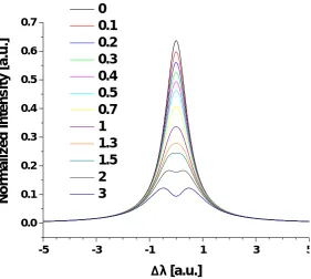
The impact of the absorption distortion on the line profile manifests in different ways depending 38
on the amount of absorption. The tendency is for the line peak to flatten and broaden indicated by 39
an increasing line width (∆λ) [13]. As the absorption becomes more extreme, the peak will take on a
40
saturated form with a clear flat top peak and as the absorption becomes even more extreme the line will 41
take on a reversed shaped with a clear central dip at the line center. This trend occurs for increasing 42
optical depthτand is displayed in Figure 1 for optical densities between 0 and 3. As can be seen,
43
for moderate absorptions the line profile may not appear distorted (seeτ=0.5 to 1). For applications
44
such as quantitative LIBS where the line shape is pivotal for determining the plasma temperature and 45
electron density [5], as well as determine elemental compositions from physical population [14] and
46
univariate/multivariate models [5,15], distortions of the line profile need to be thoroughly addressed.
47
Specific to the LIBS field of study, there is a long history of accounting for self-absorption [16–24].
48
Some methods depend on solving the equation of radiation transport[13,25–27], while others seek
49
experimental corrections to specific line shapes of interest [23].
50
- 5 - 3 - 1 1 3 5
0 . 0 0 . 1 0 . 2 0 . 3 0 . 4 0 . 5 0 . 6 0 . 7
N
o
rm
a
li
z
e
d
In
te
n
s
it
y
[a
.u
.]
D l
[ a . u . ]
0
0 . 1
0 . 2
0 . 3
0 . 4
0 . 5
0 . 7
1
1 . 3
1 . 5
2
3
Figure 1.Alterations of a Lorentzian line profile under the influence of self-absorption for increasing
optical density. The undistorted line width is 1 [a.u.].
In the present work, we detail the optical density of a laser induced plasma through out the 51
plasma decay by monitoring the temporal progression of the hydrogen Balmer seriesαline (Hα). This
52
is completed through the standard practice of using a doubling mirror to re-image the plasma onto 53
itself and take ratios of the plasma spectroscopic image collected with and without its doubled image. 54
In the following section, we detail the standard method for applying the doubling mirror method and 55
suggest a potential alternative that requires less post processing of the measured spectra. We go on 56
to apply both methods to measurements of the Hαline and use the corresponding electron density
determined from the line to indicate the usefulness of both methods of correcting the opacity of the 58
spectral line. 59
2. Theory 60
The radiation transport equation details how light can be absorbed as it passes through a dense 61
medium [11]. Specifically the amount of radiation (L(λ,x)) that leaves a column of absorbing material
62
is detailed as 63
L(λ,x) =e(λ,x)dx−κ(λ,x)Ldx, (1)
wheree(λ,x)the emission coefficient,κ(λ,x)is the absorption alongdx, anddxis a slab of absorbing
64
material. A solution to the radiation transport equation when spatial homogeneity is assumed is given 65
by 66
L(λ) =S(λ)(1−e−τ(λ))L(λ), (2)
whereS(λ)is the source function, which is taken as the ratio of the emission and absorption coefficients
67
(e(λ)/κ(λ)).L(λ)is the normalized line profile andτis the optical depth, which is defined as
68
τ(λ) =
Z `
0 κ(λ)dx, (3)
where ` is the size of the absorption path length. When the source is in local thermodynamic
69
equilibrium the source function takes the form of the Planck function [28]. In order to account
70
for absorption, one can rearrange Equation2to isolate the emission coefficient as
71
e(λ)L(λ) =L(λ) κ(λ)
1−e−τ(λ) (4)
such that if one can calculate a correction factor, apart from a multiplication of`, of the form
72
K(λ,τ) = τ
1−e−τ(λ), (5)
absorption can be taken into account along a particular line of sight in a relative manner. 73
One methods for taking absorption into account is to duplicate the emission source with reflective 74
optics and compare the original emission source to source with its duplication. In the case of laser 75
induced plasma, duplication is typically done using some optical setup using a retro-reflecting mirror 76
[8,22,23]. The retro-reflection is reduced by a factor ofe−τas it passes through the original emission
77
source such that the ratio of the reflection plus the original source to the original emission is 78
R(λ) = S(λ)(1−e
−τ+S(λ)(1−e−τG(λ)e−τ)
S(λ)(1−e−τ) , (6)
which reduces to 79
R(λ) =1+G(λ)e−τ, (7)
whereG(λ)is a term that accounts for losses along the duplication optical path length. The method
80
for tabulating a correction of the form of Equation5as outlined by Moonet al.[23] details using the
81
ratio of the continuum with and without the emission duplication as a way of avoiding determining 82
the optical losses,G(λ). This method will hereafter be referred to the Kcorr method. In this scheme the
83
correction factor is calculated as 84
K= ln(y)
with 85
y= Rc(λ)−1
R(λ)−1, (9)
whereRc(λ)is the ratio of the continuum with and without the emission duplication. Rearranging7
86
shows that the loss factor shifts the value of theτthat can be determined from direct division of the
87
measured line profiles with and without the duplication mirror. Namely, for larger losses, smallerτ’s
88
and spectral intesnites are predicted. 89
As an alternative, we suggest directly finding τ(λ) from Equation 7 as simpler method of
90
calculatingK(λ,τ) in Equation 5. This removes the need to find the ratio of the line continuum
91
and also removes the need to differentiate this continuum from the line spectrum. This alternative 92
method does however require one to provide an estimation of the losses along the optical path length 93
of the duplication imaging system. In the present work we will show that in a relative sense, the need 94
for this estimation has little impact for relative spectroscopic measurements and analyses provided all 95
lines used for analysis experience the same correction. The method will hereafter be referred to as the 96
direct method of self-absorption correction. 97
3. Experimental Details 98
Laser-induced plasma was studied spectroscopically following plasma initiation from focused 99
1064 nm, Nd:YAG laser radiation. Self-absorption effects are studied by re-imaging the plasma 100
onto itself prior to spectroscopic imaging through use of a plane, reflecting mirror. The plasma was 101
initiated by focusing 120 mJ, 14 ns pulsed laser radiation through the window of a gas cell chamber. 102
A 125-mm focal length UV-fused silica (UV-fs) planoconvex lens was used. The breakdown event 103
was imaged onto the slit of a 0.64-meter Jobin-Yvon, HR640 Czerny Turner spectrometer installed 104
with a 1200 grooves/mm grating. The gas cell was filled with 90% ultra-high purity (UHP, 99.999% 105
pure) hydrogen gas and 10% UHP nitrogen gas and was evacuated with a mechanical/diffusion pump 106
system to a pressure of 10−3Pa (1×10⁻⁵Torr) prior to filling the chamber volume with the desired gas
107
mixture atmospheres. The chamber pressure at the time of the experiment was 1.11×10⁵Pa (838 Torr).
108
The plasma emissions were recorded with an Andor iStar intensified charge couple device (ICCD). 109
The detector was a rectangular array of pixels. When coupled with the spectrometer, the horizontal 110
arrays of pixels are used to record spectrally resolved data. The vertical pixels on the detector recorded 111
spatially resolved data along the height of the spectrometer slit. The laser was focussed vertically 112
through the top of the chamber. The size of the ICCD pixels were 13.6×13.6µm. This resulted gave
113
a spectral instrument resolution of approximately 0.15 nm for the selected slit width of 50 microns. 114
Groups of 8 vertical rows were data-binned to achieve a spatial instrument resolution of 0.108 mm 115
along the slit height. The imaging characteristics of the system were such that the plasma imaged 116
onto the ICCD at a magnification of 1.05:1. The spectral and spatial resolutions (or spectral and spatial 117
instrument resolutions) are the important figures of merit, and for completeness we included the actual 118
slit width that was used. The spectral resolution is determined by the slit width, the spatial resolution 119
by the binning. Both of which are affected by the modulation transfer function, especially of the 120
intensifier. The instrument resolution is determined by analyzing the line shapes of low temperature, 121
low density stand lamp sources used for wavelength calibration. 122
Self-absorption was studied using a plane, reflecting mirror and a lens to reflect the plasma onto 123
itself prior to spectroscopic imaging. The plasma was first imaged onto the plane reflecting mirror. 124
This image was then passed back through the lens and onto the plasma. The plasma and its duplicate 125
were then imaged onto the spectrometer slit as is usually done in a typical LIBS experiment [29]. A
126
block diagram of the apparatus is shown in Figure 2. The lenses used to image the plasma onto the 127
mirror and the plasma and its duplicate image onto the spectrometer slit were identical and consisted 128
Figure 2.Block diagram of the experimental apparatus detailing self-absorption re-imaging.
the mirror and the lens used to image the plasma onto the mirror were positioned with 5-axis Gimbal 130
mounts for fine adjustments. 131
The alignment of the self-absorption apparatus is a delicate and vital component of this work 132
given the spatial resolution of the ICCD. To aid in this procedure, the lens used to image the plasma 133
with its duplication was fixed in its position so that it properly produced a focused image on the 134
spectrometer slit. This corresponded to the location equivalent to the distance of 2×the focal length
135
of the lens in relation to the spectrometer slit and 2×the back focal length (93.7 mm) in relation to
136
the breakdown plasma, when taking into account the thick-lens approximation. Likewise, the lens 137
used to image the plasma onto the plane mirror was initially placed at a distance of twice the focal 138
length of the lens in relation to the mirror and twice the back focal length of the lens in relation to the 139
breakdown plasma. The best possible alignment was achieved by fine adjustments of both lenses and 140
the mirror. The alignment was checked using zero order imaging with the spectrometer. A sufficient 141
alignment was considered to be one in which ICCD images collected with and without the duplication 142
were nearly identical. Further fine adjustments were made by comparing collected ICCD spectra with 143
and without the duplication such that the ratio was as large as possible, with an ideal ratio limit of 2. 144
These adjustments were made by viewing the Balmer series hydrogen beta line, Hβ, at a time delay of
145
10µs in SATP laboratory air breakdown. For this time delay, self-absorption for this spectral line is
146
likely to be insignificant, especially in ambient air (as differentiated from the high pressure atmosphere 147
used here) [30,31].
148
Hαspectra were recorded at systematically varied time delays starting from 10 ns following
149
plasma initiation up to a delay of 2150 ns. The selected gate width for the first 100 ns was 5 ns and a 150 150
ns gate width was used for all later measurements. Temporal resolution was achieved by synchronizing 151
the ICCD to the Q-Switch output of the laser. This image shows the spatial localization with respect 152
to the slit height and wavelength range of the emitted spectra. Though spatial resolution was used 153
for the initial measurement, all the Hαspectroscopic images were averaged after data collection to
154
improve the signal quality and mitigate the impacts of a slight misalignment on the scale of the 0.1 mm 155
spatial resolution along the vertical axis. This averaging excluded regions above and below the Hα
156
emission where only signal noise was recorded. Prior to analysis the spectrum was wavelength and 157
4. Results and Discussion 159
4.1. Temporal Self-absorption Behavior 160
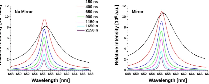
Following collection and averaging of the Hα spectra both with and without the duplicating
161
mirror, ratios of the doubled image to the non-doubled spectral image were calculated. The temporal 162
development of the Hα spectra with and without the duplicating mirror is displayed in Figures 3
163
and 4 in the first 100 ns and at the later investigated times, respectively. The left image in each figure 164
shows the spectra and the right image shows the spectra imaged with the duplication. These images 165
show the rise in the intensity of the Hαline from the spectral continuum and its growth in intensity as
166
the plasma cools and atomic recombination occurs. The spectra first become apparent after 30 ns as 167
seen in Fig 3a. The Hαline is initially very broad but narrows gradually through time as the plasma
168
decays. Prior to the 30-ns time delay, the plasma is characterized by strong continuum emissions. After 169
reaching a peak intensity between 150 and 400 ns, the line begins to decay indicating the n=3 levels of 170
the hydrogen atoms are depopulating closer to the ground level as the plasma decays further and the 171
plasma cools. 172
6 4 8 6 5 0 6 5 2 6 5 4 6 5 6 6 5 8 6 6 0 6 6 2 6 6 4 6 6 6 6 6 8
4 6 8 1 0 1 2 1 4 1 6 1 8 2 0 2 2 2 4 2 6 2 8 3 0 R e la ti v e In te n s it y [1 0 4a .u .]
W a v e l e n g t h [ n m ]
3 0 n s 4 0 n s 5 0 n s 6 0 n s 7 0 n s 8 0 n s 9 0 n s 1 0 0 n s N o M i r r o r
6 4 8 6 5 0 6 5 2 6 5 4 6 5 6 6 5 8 6 6 0 6 6 2 6 6 4 6 6 6 6 6 8
4 6 8 1 0 1 2 1 4 1 6 1 8 2 0 2 2 2 4 2 6 2 8 3 0 R e la ti v e In te n s it y [1 0 4a .u .]
W a v e l e n g t h [ n m ]
M i r r o r
Figure 3.Temporal development of the Hαline in the first 100 ns following plasma initiation. The
left image shows the measured spectra and the right image shows the spectra measured with its duplication.
6 4 8 6 5 0 6 5 2 6 5 4 6 5 6 6 5 8 6 6 0 6 6 2 6 6 4 6 6 6 6 6 8
0 2 4 6 8 1 0 1 2 R e la ti v e In te n s it y [1 0 5a .u .]
W a v e l e n g t h [ n m ]
1 5 0 n s 4 0 0 n s 6 5 0 n s 9 0 0 n s 1 1 5 0 n s 1 6 5 0 n s 2 1 5 0 n s N o M i r r o r
6 4 8 6 5 0 6 5 2 6 5 4 6 5 6 6 5 8 6 6 0 6 6 2 6 6 4 6 6 6 6 6 8
0 2 4 6 8 1 0 1 2 R e la ti v e In te n s it y [1 0 5a .u .]
W a v e l e n g t h [ n m ]
M i r r o r
Figure 4.Temporal development of the Hαline between 150 ns and 2150 ns following plasma initiation.
The left image shows the measured spectra and the right image shows the spectra measured with its duplication.
To determine the temporal profile of the self-absorption of the Hαline, the measurements with and
173
without the Hαduplication were used in conjunction with Equation 5 by two methods: 1) Equations 8
174
ratio of the continuum radiation for the Kcorr method and 2) by finding the optical depth according 176
to Equation 7 and directly substituting this into the correction factor from Equation 5 for the direct 177
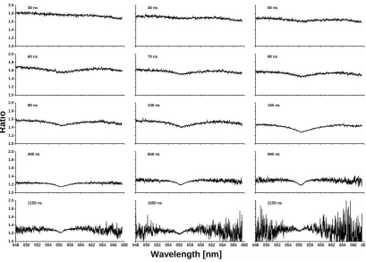
method. Both methods rely on finding the ratio of the spectra collected with and without its duplication. 178
To gain insight into the temporal development of the self-absorption, these ratios have been tracked 179
through the plasma decay and are displayed in Figure 5, showing times between 30 and 2150 ns. 180
1 . 0 1 . 2 1 . 4 1 . 6 1 . 8 2 . 0
1 . 0 1 . 2 1 . 4 1 . 6 1 . 8 2 . 0
1 . 0 1 . 2 1 . 4 1 . 6 1 . 8 2 . 0
1 . 0 1 . 2 1 . 4 1 . 6 1 . 8 2 . 0
6 4 8 6 5 0 6 5 2 6 5 4 6 5 6 6 5 8 6 6 0 6 6 2 6 6 4 6 6 6 6 6 8 1 . 0
1 . 2 1 . 4 1 . 6 1 . 8 2 . 0
6 4 8 6 5 0 6 5 2 6 5 4 6 5 6 6 5 8 6 6 0 6 6 2 6 6 4 6 6 6 6 6 8 6 4 8 6 5 0 6 5 2 6 5 4 6 5 6 6 5 8 6 6 0 6 6 2 6 6 4 6 6 6 6 6 8
3 0 n s 4 0 n s 5 0 n s
6 0 n s 7 0 n s 8 0 n s
R
a
ti
o
9 0 n s 1 0 0 n s 1 5 0 n s
4 0 0 n s 6 5 0 n s 9 0 0 n s
1 1 5 0 n s
W a v e l e n g t h [ n m ]
1 6 5 0 n s 2 1 5 0 n s
Figure 5.Ratios of the doubled Hαspectra to the non-doubled emissions through the plasma decay
from 30 ns to 2150 ns. Each image has the wavelength and ratio ranges.
Initially, at 30 ns, the ratio is quite close to 2, the theoretical limit of the ratio. When losses are 181
considered a value of the approaching or exceeding 1.8 indicates little to no line self-absorption, when 182
the signal almost entirely a continuum signal. This would be consistent with a plasma model in 183
which the approach atomic levels of hydrogen (n=2 and n=3 for the Balmerαline) are just beginning
184
to populate. As the plasma decay continues these levels become more populated, as evidenced by 185
the rise in intensity of the Hα line. As this goes on, the ratio of the Hα line with and without its
186
duplication begins to steadily decrease. By 100 ns the value of the ratio is approximately 1.6 and 187
reaches a maximum low of about 1.3 to 1.25 at time later than 400 ns. After this time, there is an 188
apparent rise the ratio indicating the amount of extinction along the optical line of sight is reducing. 189
However, the plateau in the decay of the ratio more than likely indicates that a limit in the sensitivity 190
of the technique has been reached. 191
Figure 5 also shows the tendency for the line center to be more perturbed by self-absorption, as 192
was shown in Figure 1. As the line absorption becomes more prominent, a dip in the ratio begins 193
to appear near theHαline center. This is first seen in at a time of 60 ns and grows in prominence as
194
the plasma decays. The magnitude of the dip relative the mostly constant ratio in the line wings is 195
between 0.05 to 0.1. Thus a minimum ratio of approximately 1.15 at the line center can be seen for the 196
400 ns time delay. 197
As the plasma decays, the line becomes more susceptible to experimental noise. The impact of 198
this is amplified by dividing two spectra giving rise to the extreme noise seen in the ratios calculated 199
after 800 ns. This noise addition can also be attributed to the narrowing nature of the Hαline as the
wings of the later time ratios are most impacted. In this case the wings represent a part of the spectrum 201
that is characterized by an also decaying spectral continuum that will largely be the same between 202
spectra collected with and without the duplication. Furthermore, this weakly intense continuum is 203
more susceptible to noise contributions which is further amplified when the ratio is taken. This would 204
also manifest in the early investigated times prior to 150 ns, the Hαline has contributions beyond
205
the spectral range of our instrument, making it difficult to asses the contributions of the continuum 206
radiation. 207
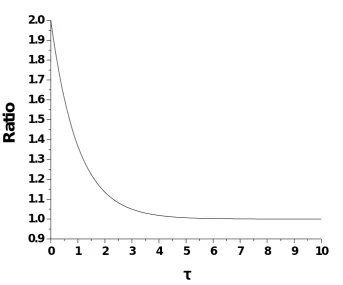
As a reference, Figure 6 shows the relationship between optical depth and the ratio of the spectral 208
line with and without its duplication and without any losses given by Equation 5. At zero optical 209
depth, the ratio is 2. As the optical depth increases to values greater than 1 (τ= 1 is often cited as being
210
optically thick [11]) the ratio approaches a limit of 1 indicating no radiation has emerged from the
211
source. An optical depth of 1 corresponds to a ratio of nearly 1.37. Figure 5 suggests that a ratio of 1.25 212
in the line wings and 1.15 at line center can be extracted. This corresponds to optical depths of 1.38 and 213
1.89 at the line wings and line center, respectively, when no losses are considered. This is however an 214
idealization that doesn’t match the experimental conditions. If one were to assume a modest amount 215
of loss along the duplication optical path length, such as 20% which means there is 93% transmittance 216
all interfaces along duplication optical path, the optical depths become 1.16 and 1.67 at the line wings 217
and line center, respectively. With a loss of 20% the ratio of 1.8 corresponds to an optically thin source. 218
The increase in self-absorption as the plasma cools and decays has been reported in other studies as 219
well [21,32,33]. 220
Discussions of self-reabsorption [34] indicate that for an optically thin plasma and an ideal
221
doubling mirror in place, the transmitted intensity amounts to twice that without the mirror. However, 222
when the plasma is optically thick (at line centerκ0x1) and for a Voigt parameter,a, or the ratio of
223
Lorentzian and of Gaussian widths,a1, the line absorption,AL, amounts toAL =2−
√
2=0.59.
224
In other words, the transmission equals√2, i.e., 1.41 is the limiting value for the transmission. This
225
results has been extensively communicated [35] and applied in the modeling of flame experiments [36]
226
that utilize an experimental arrangement comprised of two consecutive line sources. 227
4.2. Self-absorption Impact on Line Shapes 228
The impact of the self-absorption on the temporal development is further discussed by applying 229
the correction factor given in Equation 5 in two ways. The first is to use the Kcorr method outlined 230
by Moonet al.[23]. In performing this method, the ratios from Figure 5 are used but they have been
231
smoothed with a second order Savitzky-Golay filter with a window size of 50 in order to reduce the 232
impact of noise on the corrected spectra. The ratio of the continuum was estimated by averaging 233
the spectral end points on the desired range. These points were 645.5 and 667.547 nm. When theHα
234
line is sufficiently narrow (∆λ = 4nm) these points indicate a distance from line center that is 5×
235
the line width, which provides a reasonable continuum estimation that is uninhibited by the Hαline
236
profile. When the line is at its widest, these points are only 2×the line width which introduces some
237
uncertainty in determining the ratio of the continuum and also represents a limit of this method for 238
narrow band spectra with broad spectral features. 239
The second method of correction is directly invert Equation 7 to find the optical depth using 240
the ratios given in Figure 5 for the direct method. The ratios are once again smoothed using the 241
Savitzky-Golay filter. With this method one either needs to have an accurate characterization of the 242
optical losses along the duplication optical path length or assume a reasonable loss. Characterizing 243
the loss along duplication optical path length could be an arduous task that involves considering the 244
modulation transfer function and other geometric optics impacts to determine the imaging system 245
quality. At this stage, rather than take on this task, we instead consider three values of a loss to gauge 246
the efficacy of using this method to correct theHαspectra in a relative sense. The losses we consider
247
0
1
2
3
4
5
6
7
8
9
1 0
0 . 9
1 . 0
1 . 1
1 . 2
1 . 3
1 . 4
1 . 5
1 . 6
1 . 7
1 . 8
1 . 9
2 . 0
R
a
ti
o
t
Figure 6.Relationship between optical depth,τ, and the ratio of a spectral line with its duplication
compared to the line without duplication.
correspond to constantG(λ)values of 1, 0.9, and 0.8. It is also reasonable to assume that the loss on a
249
narrow spectral band of 22 nm is relatively constant. 250
Using three different values of the loss allows us to see how the line shape is impacted changing 251
this parameter which will be important for further studies using this method of self-absorption 252
correction. The no loss and 10% loss cases are likely ideal scenarios that would be difficult to 253
experimentally achieve. The 20% loss case represents a best case scenario in which the optical system is 254
perfectly aligned and highly efficient optics at the Hαwavelength are considered with a transmittance
255
near 0.93 at each optical interface on the duplication optical path. After the loss is accounted for, the 256
line profiles are now corrected using Equation 5 with the tabulated optical depths. 257
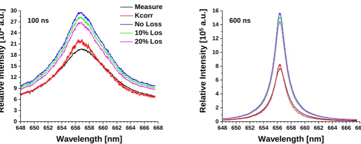
Figure 7 shows the result of applying both methods of correcting the Hαline at 100 and 600 ns time
258
delays. For comparison, the measured line profile without its duplication is also presented. The most 259
notable aspect of applying the two different methods is the Kcorr method produces a spectrum that is 260
more comparable in intensity with the original line profile, however, the corrected line profile is now 261
narrower (at both time delays) as would be expected. When the direct method as the self-absorption 262
correction, the line intensity grows. The amount of intensity growth depends on the amount of loss. 263
The greater the loss, the less the intensity of the line grows. The spectral features for each of the 264
considered losses do appear to be narrower after correction, however. 265
Despite the line growth when the lines are corrected according to the direct method, the spectral 266
intensities that are observed are relative in nature, as only a relative intensity correction of the 267
experimental apparatus was performed. This is a common practice as absolute calibrations of spectral 268
imaging systems are difficult to perform and are not necessary in most cases since quantitative 269
information can be extracted from a relative intensity correction. For example, the line shape would 270
only be impacted by an amplitude factor. Provided this amplitude factor is self consistent across an 271
6 4 8 6 5 0 6 5 2 6 5 4 6 5 6 6 5 8 6 6 0 6 6 2 6 6 4 6 6 6 6 6 8 0 3 6 9 1 2 1 5 1 8 2 1 2 4 2 7 3 0 R e la ti v e In te n s it y [1 0 4a .u .]
W a v e l e n g t h [ n m ]
M e a s u r e d K c o r r N o L o s s 1 0 % L o s s 2 0 % L o s s 1 0 0 n s
6 4 8 6 5 0 6 5 2 6 5 4 6 5 6 6 5 8 6 6 0 6 6 2 6 6 4 6 6 6 6 6 8
0 2 4 6 8 1 0 1 2 1 4 1 6 R e la ti v e In te n s it y [1 0 5a .u .]
W a v e l e n g t h [ n m ]
6 0 0 n s
Figure 7.Results of correcting the Hαspectrum using the methods of Equation 8 and 9 and also directly
calculating the optical depth with assumed losses in conjunction with Equation 7 for 100 ns (left) and 400 ns (right) time delays in the plasma decay.
be applied to multiple lines self consistently, further methods should not be impacted, though one 273
should perform a baseline study for each new type of analysis that is considered (Boltzmann plots, 274
multivariate modeling,etc.).
275
To compare the two methods of self-absorption correction and verify the line profile remain 276
unaltered regardless of the method, the uncorrected and corrected line profiles were fit in order to 277
calculate the line width. The line width was used to calculate the electron density to see the impact on 278
determining the plasma state. The line profiles were fit with a Voigt line profile, an integral line shape 279
function resulting from the convolution of Lorentzian and Gaussian line shapes [11]. The Lorentzian
280
component of the Voigt profile represents the Stark broadened Hαline, while the Gaussian component
281
represents in the instrument function width of 0.15 nm (determined during spectrometer-detector 282
calibration) under the assumption of negligible Doppler broadening. One should note that the exact 283
line shape of a Stark broadened hydrogen Balmer series line is a Holtsmarkian line profile, however 284
for ease of analysis the Lorentzian line profile is an acceptable approximation [37–39].
285
The integral Voit line profile is numerical calculated using Fadeeva function or also called complex 286
complimentary error function with the fixed Gaussian width of 0.15 nm [40,41]. The line profile fitting
287
was implemented in the MatLab scripting environment [42]. The Fadeeva function was numerically
288
calculated using the Algorithm 916 method of Zaghloulet al.[43]. Line shape fitting was carried using
289
a Trust Region nonlinear curve fitting routine [44,45] in which the fit parameters were the line width,
290
amplitude, and shift as well as two terms used characterize a linear offset to model any continuum 291
components in the spectra signals. 292
In terms of characterizing the electron density of the plasma, one typically uses the line width. 293
As a result, the behavior of the width before and after the self-absorption corrections is considered. 294
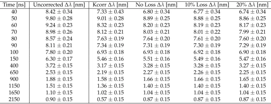
These results are displayed in Table 1 and detail the line width progression from 40 ns to 2150 ns. The 295
30 ns time is left out from this discussion because the Hαline has not yet emerged from the spectral
296
continuum. The table shows the what the uncorrected line width would be and the corrected line 297
widths using The Kcorr and direct methods with no, 10%, and 20% losses. The table shows that initially 298
the Hαline is very broad (∆λ>9 nm) and subsequently decays to a relatively narrow line (∆λ<1 nm).
299
The uncertainties on the indicated line widths represent contributions from both the minimum spectral 300
resolution and uncertainties introduced during line profile fitting. These uncertainties are greatest 301
when the line is at its broadest and decay to a minimum value of 0.15 nm representing little to no 302
uncertainty contribution from the fitting algorithms. This occurs after 400 ns when the line width is 303
less than 4 nm and 5×the line width occurs on the investigated spectral range, indicating the spectral
304
continuum is likely to be well characterized within the measurement. 305
Table 1 shows that regardless of the method of correcting the spectrum, the line width is reduced 306
Table 1.Line widths of the Hαline prior to and after self-absorption correction using all the stated
methods. The 30 ns time delay is excluded form the table because the Hαhas not yet emerged from the
continuum at this point.
Time [ns] Uncorrected∆λ[nm] Kcorr∆λ[nm] No Loss∆λ[nm] 10% Loss∆λ[nm] 20%∆λ[nm]
40 8.42±0.34 7.33±0.43 6.80±0.34 6.77±0.34 6.74±0.34
50 9.80±0.28 9.01±0.28 8.89±0.25 8.88±0.25 8.86±0.25
60 9.24±0.23 8.32±0.23 8.20±0.23 8.19±0.23 8.17±0.23
70 8.98±0.26 8.12±0.21 8.03±0.21 8.01±0.22 7.99±0.21
80 8.57±0.24 7.63±0.19 7.64±0.20 7.61±0.20 7.60±0.20
90 8.11±0.21 7.34±0.19 7.31±0.19 7.30±0.19 7.29±0.19
100 7.80±0.20 6.93±0.18 6.93±0.18 6.92±0.18 6.90±0.18
150 6.30±0.17 5.46±0.16 5.51±0.16 5.49±0.16 5.47±0.16
400 3.72±0.15 3.17±0.15 3.28±0.15 3.28±0.15 3.27±0.15
650 2.53±0.15 2.19±0.15 2.27±0.15 2.26±0.15 2.25±0.15
900 1.88±0.15 1.58±0.15 1.66±0.15 1.66±0.15 1.65±0.15
1150 1.51±0.15 1.36±0.15 1.40±0.15 1.40±0.15 1.40±0.15
1650 1.10±0.15 1.02±0.15 1.04±0.15 1.04±0.15 1.04±0.15
2150 0.90±0.15 0.57±0.15 0.87±0.15 0.87±0.15 0.87±0.15
from the early times to the later plasma decay times, respectively. Furthermore, the two methods of 308
correcting for the self-absorption return similar values of the line width after correction. The amount 309
of loss considered in the relative correction model also produces similar line widths. Early in the 310
plasma decay the Kcorr methods tends produce line widths that are 0.1 nm greater than the Equation 7 311
method. This can be attributed to the difficulty in appropriately finding the continuum ratio when the 312
line is still very broad. 313
When the uncertainties are considered, the line widths can be considered to be the same for both 314
methods of self-absorption correction and all three losses considered. There are two exceptions when 315
the Kcorr value does not match the direct method. At 40 ns, the Kcorr method is 0.5 nm greater, yet 316
there is a slight overlap when the uncertainties are considered. At this time, the Hα, while noticeable,
317
is still emerging from the continuum and is also very broad making it difficult to ascertain the ratio of 318
the continuum. This point was also the most uncertain in terms of the line profile fitting. The second 319
point with a notable discrepancy is the 2150-ns time delay value for Kcorr. At this time the value of 320
the ratio of the continuum is also difficult to ascertain due to the decaying nature of the plasma. As 321
the plasma decays this value will tend toward unity which causes a singularity in the expression for 322
Kcorr in Equation 8. This represents and advantage of the method using Equation 7 directly, as less 323
processing of the spectra is required in order to obtain a correction factor. With the fact that the line 324
profile is preserved in a relative sense one may prefer this method even though an estimate of the loss 325
along the duplication optical path is required. 326
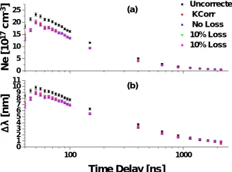
The final investigation of this work is to consider the electron density, Ne, decay of the plasma.
327
This is shown in Figure 8 along with the line width decay of the Hα line. The Ne was determined
328
Hα line width using the empirical formula outlined in Reference [46]. For the Hα line, the Ne is
329
approximately proportional to∆λ2/3[37,38,46,47]. This figure mimics the results shown in Table 1.
330
The line widths and electron densities are reduced when each of the self-absorption correction methods 331
are applied and the each of the corrected densities and line widths agree with each other, especially 332
when the uncertainty is considered. The impact of not accounting for self-absorption, even when 333
moderate is clear from Figure 8. The electron density can be over estimated. For quantitative analysis, 334
such as calibration free LIBS, this can alter the elemental compositions that are determined, over and 335
beyond any impact that the line shape distortion may cause. Also as expected, the plasma is seen 336
decay in density as the plasma cools and atomic and molecular recombination occurs. The plasma 337
is seen to decay from an electron density of approximately 2×1018 cm−3at 50 ns to approximately
338
5×1016cm−3at 2150 ns, following some manner of exponential decay as one might expect.
0
5
1 0 1 5 2 0 2 5
1 0 0 1 0 0 0
0
1
2
3
4
5
6
7
8
9
1 0 1 1
U n c o r r e c t e d
K C o r r
N o L o s s
1 0 %
L o s s
1 0 %
L o s s
N
e
[1
0
1
7
c
m
-3
]
( a )
Dl
[n
m
]
T i m e D e l a y [ n s ]
( b )
Figure 8.Decay of the plasma(a)electron density and(b)Hαline width through time.
5. Conclusions 340
In this work, the temporal development of the self-absorption of the Hαline was considered by
341
studying the duplication method of re-imaging the spectral line onto itself and comparing the line 342
with and without this duplication. The temporal development of this ratio indicated that the early 343
stages of the plasma decay there is little self-absorption occurring in the plasma as the ratio value 344
was 1.8. Throughout the plasma decay this value reduced to a minimum of 1.25 indicating an optical 345
depth of 1.16 when a loss of a 20% is considered along the duplication optical path length. This result 346
showed that as the plasma decayed and cooled the appropriate levels of hydrogen became sufficiently 347
populated to induce self-absorption of the spectral line even if it is not readily obvious via visual 348
inspection of the line profile. 349
The spectral line profiles were then corrected using two methods. The first was the standard 350
method outlined by Moonet al.[23]. The second involved a direct calculation of the optical depth from
351
the ratios of the spectra measured with and without its duplication. This required the assumption of 352
some form of loss along the duplication optical path length. Investigation of the corrected profiles 353
using line profile fitting methods with an emphasis on preserving the line width showed that both 354
methods corrected the line self-absorption equally by finding the same line width within experimental 355
uncertainty. The amount of loss considered along the duplication optical path only impacted the 356
intensity of the signal, such that in an experiment where only relative intensities are required either 357
method of self-absorption correction may be considered. 358
Author Contributions:All authors contributed equally to this work.
359
Funding:This research received no external funding.
360
Acknowledgments:The authors wish to acknowledge the support of the Center for Laser Applications at the
361
University of Tennessee Space Institute for partial support of the experimental work of this effort.
362
Conflicts of Interest:The authors declare no conflict of interest.
References 364
1. Parigger CG. Atomic and molecular emissions in laser-induced breakdown spectroscopy. Spectrochim. Acta
365
Part B: At. Spectrosc. 2013;79-80:4 – 16.
366
2. Harilal SS, Brumfield BE, Cannon BD, Phillips MC. Shock wave mediated plume chemistry for molecular
367
formation in laser ablation plasmas. Anal. Chem. 2016;88:2296–2302.
368
3. Lam J, Amans D, Chaput F, Diouf M, Ledoux G, Mary N, Masenelli-Varlot K, Motto-Ros V, Dujardin C.
369
γ-Al2O3nanoparticles synthesized by pulsed laser ablation in liquids: A plasma analysis. Phys. Chem.
370
Chem. Phys. 2016;16:963–973.
371
4. Panda AK, Singh A, Thirumurugesan R, Kuppusami P, Mohandas E. Optimization of substrate-target
372
distance for pulsed laser deposition of tungsten oxide thin films using Langmuir probe. J. Instrument.
373
2015;10(09):P09014.
374
5. Cremers DA, Radziemski LJ. Handbook of Laser-Induced Breakdown Spectroscopy. Hoboken, NJ: John
375
Wiley and Sons; 2006.
376
6. Hahn DW, Omenetto N. Laser-Induced Breakdown Spectroscopy (LIBS), Part 1: Review of Basic Diagnostics
377
and Plasma-Paritcle Interactions: Still-Challeneging Issues Within the Analytical Plasma Community. Appl.
378
Spectrosc. 2010;64:335A–366A.
379
7. Hahn DW, Omenetto N. Laser-Induced Breakdown Spectroscopy (LIBS), Part II: Review of Instrumental
380
and Methodological Approaches to Material Analysis and Applications to Different Fields. Appl. Spectrosc.
381
2012;66:347–419.
382
8. Konjevic N. On the use of non-hydrogenic spectral line profiles for plasma electron density diagnostics.
383
Plasma Sources Sci. Technol. 2001;10:356–363.
384
9. Konjevic N, Dimitrijevic MS, Wiese WL. Experimental stark widths and shifts for spectral lines of neutral
385
atoms: A critical review of selected data for the period 1976 to 1982. J. Phys. Chem. Ref. Data.
386
1984;13:649–686.
387
10. Konjevic N, Dimitrijevic MS, Wiese WL. Experimental stark widths and shifts for spectral lines of positive
388
ions: A critical review of selected data for the period 1976 to 1982. J. Phys. Chem. Ref. Data. 1984;13:619–647.
389
11. Kunze HJ. Introduction to Plasma Spectroscopy. Berlin, Heidelberg: Springer-Verlag; 2009.
390
12. Griem HR. Spectral Line Broadening By Plasmas. New York: Academic Press; 1974.
391
13. Cowan RD, Dieke GH. Self-Absorption of Spectrum Lines. Rev. Mod. Phys. 1948;20:418–455.
392
14. Cristoforetti G, Giacomo AD, Dell’Aglio M, Legnaioli S, Tognoni E, Palleschi V, Omenetto N. Local
393
Thermodynamic Equilibrium in Laser-Induced Breakdown Spectroscopy: Beyond the McWhirter criterion.
394
Spectrochim. Acta Part B: At. Spectrosc. 2010;65:86 – 95.
395
15. Gottfried JL. Discrimination of biological and chemical threat simulants in residue mixtures on multiple
396
substrates. Anal. Bioanal. Chem. 2011;400(10):3289–3304.
397
16. Amamou H, Bois A, Ferhat B, Redon R, Rossetto B, Matheron P. Correction of self-absorption spectral line
398
and ratios of transition probabilities for homogeneous and LTE plasma. J. Quant. Spectrosc. Radiat. Transf.
399
2002;75(6):747 – 763.
400
17. Amamou H, Bois A, Ferhat B, Redon R, Rossetto B, Ripert M. Correction of the self-absorption for
401
self-reversed spectral lines: Application to two resonance lines of nuetral aluminium. J. Quant. Spectrosc.
402
Radiat. Transf. 2003;77:362–372.
403
18. Bulajic D, Corsi M, Cristoforetti G, Legnaioli S, Palleschi V, Salvetti A, Tognoni E. A procedure for correcting
404
self-absorption in calibration free-laser induced breakdown spectroscopy. Spectrochim. Acta Part B: At.
405
Spectrosc. 2002;57:339 – 353.
406
19. Burger M, Sko˘ci´c M, Bukvi´c S. Study of self-absorption in laser induced breakdown spectroscopy.
407
Spectrochim. Acta Part B: At. Spectrosc. 2014;101:51 – 56.
408
20. El Sherbini AM, El Sherbini TM, Hegazy H, Cristoforetti G, Legnaioli S, Palleschi V, Pardini L, Salvetti A,
409
Tognoni E. Evaluation of self-absorption coefficients of aluminum emission lines in laser-induced breakdown
410
spectroscopy measurments. Spectrochim. Acta Part B. At. Spectrosc. 2005;60:1573–1579.
411
21. Fu Y, Warren RA, Jones WB, Smith BW, Omenetto N. Detecting Temporal Changes of Self-Absorption
412
in a Laser-Induced Copper Plasma from Time-Resolved Photomultiplier Signal Emission Profiles. Appl.
413
Spectrosc. 2019;73(2):163–170.
22. Herrera KK, Tognoni E, Omenetto N, Smith BW, Winfordner JD. Semi-quantitative analyis of metal alloys,
415
brass and soil samples by calibration-free laser-induced breakdown spectroscopy: Recent results and
416
considertions. J. Anal. At. Spectrom. 2009;24:413–425.
417
23. Moon HY, Herrera KK, Omenetto N, Smith BJ, Winefordner JD. On the usefulness of a duplicating mirror
418
to evaluate self-absorption effects in laser induced breakdown spectroscopy. Spectrochim. Acta Part B: At.
419
Spectrosc. 2009;64:702–713.
420
24. Omenetto N, Winefordner JD, Alkemade CTJ. An expression for the atomic flourescence and
421
thermal-emission intensity under conditions of near saturation and arbitrary self-absorption. Spectrochim.
422
Acta Part B: At. Spectrosc. 1975;30:335–341.
423
25. Hermann J, Grojo D, Axente E, Gerhard C, Burger Mcv, Craciun V. Ideal radiation source for plasma
424
spectroscopy generated by laser ablation. Phys. Rev. E. 2017;96:053210.
425
26. Gornushkin IB, Stevenson CL, Smith BW, Omenetto N, Winefordner JD. Modeling an inhomogeneous
426
optically thick laser induced plasma: a simplified theoretical approach. Spectrochim. Acta Part B: At.
427
Spectrosc. 2001;56(9):1769 – 1785.
428
27. Hermann J, Boulmer-Leborgne C, Hong D. Diagnostics of the early phase of an ultraviolet laser induced
429
plasma by spectral line analysis considering self-absorption. J. Appl. Phys. 1998;83(2):691–696.
430
28. Bransden BH, Joachain CJ. Physics of atoms and molecules. 2nd ed. New York: Prentice Hall; 2003.
431
29. Parigger CG, Woods AC, Witte MJ, Swafford LD, Surmick DM. Measurement and analysis of atomic
432
hydrogen and diatomic molecular AlO, C2, CN, and TiO spectra following laser-induced optical breakdown.
433
J. Vis. Exp. 2012;38:E51250.
434
30. Ivkovi´c M, Konjevi´c N, Pavlovi´c Z. Hydrogen Balmer beta: The separation between line peaks for plasma
435
electron density diagnostics and self-absoprtion test. J. Quant. Spectrosc. Radiat. Transf. 2015;154:1–8.
436
31. Gautm G, Surmick DM, Parigger CG. Comment on "Hydrogen Balmer beta: The separation between line
437
peaks for plasma electron density diagnsotics and self-saborption test". J. Quant. Specrosc. Radiat. Transf.
438
2015;160:19–21.
439
32. Aguilera JA, Aragón C. Characterization of laser-induced plasmas by emission spectroscopy with
440
curve-of-growth measurements. Part I: Temporal evolution of plasma parameters and self-absorption.
441
Spectrochim. Acta Part B: At. Spectrosc. 2008;63:784 – 792.
442
33. Gornushkin IB, Anzano JM, King LA, Smith BW, Omenetto N, Winefordner JD. Curve of growth methodology
443
applied to laser-induced plasma emission spectroscopy. Spectrochim. Acta Part B: At. Spectrosc.
444
1999;54(3):491 – 503.
445
34. Fujimoto T. Plasma Spectroscopy. Oxford: Clarendon-Press; 2004.
446
35. Ladenburg R, Reiche F. Über selective Absorption. Ann. Phys. 1913;347(11):181 – 209.
447
36. Gouy GL. Recherches Photométrigues sur les Flammes Colorées. Ann. Chim. Phys. 1879;18(5):5 – 101.
448
37. Gigosos MA, Gonzalez MA, Cardenoso V. Computer simulated Balmer-alpha, -beta, and -gamma Stark line
449
profiles for non-equilibirum plasma diagnostics. Spectrochim. Acta Part B: At. Spectrosc. 2003;58:1489–1504.
450
38. Konjevi´c N, Ivkovi´c M, Sakan N. Hydrogen Balmer lines for low electron number density plasma diagnostics.
451
Spectrochim. Acta Part B: At. Spectrosc. 2012;76:16 – 26.
452
39. Parigger CG, Plemmons DH, Oks E. Balmer series Hβmeasurements in a laser-induced hydrogen plasma.
453
Appl. Opt. 2003;42(30):5992–6000.
454
40. Abramowitz M, Stegun IA. Handbook of mathematical functions with formulas, graphs, and mathematical
455
tables. 9th ed. New York: Dover; 1964.
456
41. Fadeeva V, Terentjev NM. Tables of values of the proability integral for complex arguments. Moscow: State
457
Publishing House for Technical and Technological Literature; 1954.
458
42. MatLab 2018a TM. Natick, MA; 2018.
459
43. Zaghloul MR, Ali AN. Algorithm 916: Computing the Faddeyeva and Voigt functions. ACM Trans. Math.
460
Soft. 2011;38:15:1–15:22.
461
44. Byrd RH, Schnabel RB, Schultz GA. A trust region algorithm for nonlinearly constrained optimization.
462
SIAM J. Numer. Anal. 1987;24:1152–1170.
463
45. Coleman TF, Li Y. An Interior Trust Region Approach for Nonlinear Minimization Subject to Bounds. SIAM
464
J. Optimiz. 1996;6:418–445.
465
46. Surmick DM, Parigger CG. Empirical Formulae for Electron Density Diagnostics from Hαand HβLine
466
Profiles. Int. Rev. At. Mol. Phys. 2014;5:73–81.
47. Griem HR, Halenka J, Olchawa W. Comparison of hydrogen Balmer-alpha Stark profiles measured at high
468
electron densities with theoretical results. J. Phys. B: At. Mol. Opt. Phys. 2005;38(7):975.