Using Variance to Analyze Visual Cryptography Schemes
∗Teng Guo1,2, Feng Liu1, ChuanKun Wu1 and YoungChang Hou3 1State Key Laboratory of Information Security
Institute of Information Engineering, Chinese Academy of Sciences, Beijing, China 2Graduate University of Chinese Academy of Sciences, Beijing 100190, China
3Department of Information Management, Tamkang University
Taipei County 251, Taiwan
Email: {guoteng,liufeng,ckwu}@is.iscas.ac.cn, [email protected]
Abstract
A visual cryptography scheme (VCS) is a secret sharing method, for which the secret
can be decoded by human eyes without needing any cryptography knowledge nor any
com-putation. Variance is first introduced by Hou et al. in 2005 and then thoroughly verified
by Liu et al. in 2012 to evaluate the visual quality of size invariant VCS. In this paper, we
introduce the idea of using variance as an error-detection measurement, by which we find
the security defect of Hou et al.’s multi-pixel encoding method. On the other hand, we find
that variance not only effects the visual quality of size invariant VCS, but also effects the
visual quality of VCS. At last, average contrast associated with variance is used as a new
criterion to evaluate the visual quality of VCS.
Keywords: Visual cryptography, Secret sharing, Variance, Error-detection, Visual quality
1
Introduction
Naor and Shamir first introduced the concept of k out of n threshold visual cryptography scheme ((k, n)-VCS) [9], which splits a secret image into n shares in such a way that the stacking of any kshares can reveal the secret image but any less than k shares should provide no information (in the information-theoretic sense) of the secret image, except the size of it. Ateniese et al. extended the model of Naor and Shamir to general access structure in [1]. Suppose the participant set is denoted as P = {1,2,3, . . . , n}, a general access structure is a specification of qualified participant sets ΓQual∈2P and forbidden participant sets ΓF orb ∈2P.
Any participant set X∈ΓQual can reveal the secret by stacking their shares, but any participant
set Y∈ ΓF orb cannot obtain any information of the secret image. In (k, n) threshold access
structure, ΓQual={B ⊆P :|B| ≥k} and ΓF orb ={B ⊆P :|B| ≤k−1}.
Ito et al. and Yang separately introduced size invariant visual cryptography scheme (SIVCS) in [10] and [13] respectively, which has no pixel expansion. In SIVCS, both white and black pixels
∗This work was supported by NSFC No.60903210.
can be recovered as black, which results in deteriorated visual quality compared to VCS. To improve SIVCS’s visual quality, Hou et al. proposed the multi-pixel encoding method (MPEM) in [5]. Compared to VCS (see [9] and [1]), the main advantage of SIVCS and MPEM is that they are both of no pixel expansion, while the best pixel expansion of VCS is exponential large (e.g. the best pixel expansion of (n, n)-VCS is 2n−1).
Variance is first introduced by Hou et al. in [5] to evaluate the visual quality of the recovered image of SIVCS. Liu et al. thoroughly verify, analytically and experimentally, the effectiveness of the criterion in [7]. In this paper, we first introduce the idea of using variance as an error-detection measurement, by which we find the security defect of Hou et al.’s MPEM that for secret image with simple contours, its content can be perceived from any single share. On the other hand, we find that variance not only effects the visual quality of SIVCS, but also effects the visual quality of VCS. At last, average contrast associated with variance is used as a new criterion to evaluate the visual quality of VCS.
This paper is organized as follows. In Section 2, we give some preliminaries of VCS. In Section 3, we use variance as an error-detection measurement. In Section 4, we use average contrast and variance to evaluate the visual quality of VCS. The paper is concluded in Section 5.
2
Preliminaries
In this section, we first give the definition of VCS. Then we give a brief description of the MPEM proposed by Hou et al. in [5].
Before moving any further, we first set up our notations. Let X be a subset of{1,2,· · · , n} and let |X| be the cardinality of X. For any n×m Boolean matrix M, let M[X] denote the matrixM constrained to rows ofX, thenM[X] is a|X|×mmatrix. We denote byH(M[X]) the Hamming weight of theOR result of rows ofM[X]. Let C0 andC1 be two collections ofn×m Boolean matrices, we defineC0[X] ={M[X] :M ∈C0}, and defineC1[X] ={M[X] :M ∈C1}. In a visual cryptography scheme (VCS) with n participants, we share one pixel at a time, which is either white or black. If the pixel to be shared is white (resp. black), we randomly draw a share matrix from C0 (resp. C1) and distribute the j-th (1 ≤j ≤ n) row to share j, where 0 denotes a white pixel and 1 denotes a black pixel. A VCS for an access structure Γ is defined as follows:
Definition 1 (VCS [1]) The two collections of n×m Boolean matrices (C0, C1) constitute a
({ΓQual,ΓF orb}, m, n)-VCS if the following conditions are satisfied:
1. (Contrast)For any participant set X∈ΓQual, we denotelX = max M∈C0[X]
H(M), and denote
hX = min M∈C1[X]
H(M). It holds that0≤lX < hX ≤m.
2. (Security) For any participant set Y∈ΓF orb,C0[Y]andC1[Y]contain the same matrices with the same frequencies.
1. (Contrast) α = min
X∈ΓQual
αX, whereαX =
hX −lX
m . The relative difference in Hamming weight between two recovered blocks of a black pixel and a white pixel in the original image. This represents the loss in contrast. We would likeα to be as large as possible.
2. (P ixel expansion) m, the number of pixels in a share that is encoded from a pixel in the original image. This represents the loss in resolution and the expansion in share size. We would like mto be as small as possible.
3. (Randomness) |C0| and |C1|, the size of collections C0 and C1. log2|C0| and log2|C1| represent the number of random bits needed to share a white and black pixel respectively and do not affect the visual quality of the recovered image.
4. (Average Contrast) ¯α= min
X∈ΓQual
¯
αX, where ¯lX =
∑
M∈C0[X]
H(M)
|C0[X]|and ¯hX = ∑
M∈C1[X]
H(M) |C1[X]|
and ¯αX =
¯ hX −¯lX
m . The relative difference in average Hamming weight between two re-covered blocks of a black pixel and a white pixel in the original image. This represents the loss in average contrast. We would like ¯α to be as large as possible.
5. (V ariance) ¯σ = min
X∈ΓQual
¯
σX and ¯σ′ = min X∈ΓQual
¯
σX′ , where ¯σX =
∑
M∈C0[X]
(H(M)−¯lX)2
|C0[X]|
and ¯σX′ = ∑
M∈C1[X]
(H(M)−¯hX)2
|C1[X]| . The variation of Hamming weights of the recovered block of a white pixel (resp. a black pixel) in the original image. We would like ¯σ and ¯σ′ to be as small as possible.
We would like to point out that the first three parameters are the commonly accepted evaluation criteria of VCS, while ”Average Contrast” is a parameter generalized from SIVCS and we use it to overcome the weaknesses of the parameter ”Contrast”, as will be discussed in Section 4.
If the two collections of n×mBoolean matrices (C0, C1) can be obtained by permuting the columns of the corresponding n×m Boolean matrix (S0 forC0, andS1 for C1) in all possible ways, we will call the twon×m Boolean matrices the basis matrices, which is widely used in VCS, see [1–3, 6, 9, 11]. In this case, the size of the collections (C0, C1) is the same (both equal tom!). A ({ΓQual,ΓF orb}, m, n)-VCS based on basis matrices is defined as follows:
Definition 2 (VCS based on basis matrices [1]) The twon×mBoolean matrices(S0, S1)
constitute a ({ΓQual,ΓF orb}, m, n)-VCS if the following conditions are satisfied:
1. (Contrast) For any participant set X ∈ ΓQual, we denote lX = H(S0[X]), and denote hX =H(S1[X]). It holds that0≤lX < hX ≤m.
2. (Security) For any participant set Y ∈ΓF orb, S0[Y] and S1[Y]are equal up to a column
S0 and S1 are also referred to as the white and black basis matrices respectively. In a SIVCS [10, 13], to share a black (resp. white) pixel, we randomly choose a column from the black (resp. white) basis matrix, and then distribute the i-th row of the column to participant i. In a ({ΓQual,ΓF orb}, n)-SIVCS, considering qualified participant setX∈ΓQual, a black pixel
is recovered as black with probability hX
m, which is higher than the probability lX
m that a white
pixel is recovered as black. Hence we can perceive the secret from the overall view. However, SIVCS does not satisfy that there is a gap between the Hamming weights of the recovered blocks of a black pixel and that of a white pixel as VCS does, because in SIVCS both black and white pixels can be recovered as black. The average contrast of qualified participant setX is defined as ¯αX =
hX−lX
m and the average contrast of the scheme is defined as ¯α=X∈minΓQual
¯ αX.
In the following, the MPEM proposed by Hou et al. in [5] is described as Construction 1 for convenience, which encrypts multiple pixels (nonadjacent for most cases) simultaneously.
Construction 1 Let M0 (resp. M1) be the n×r white (resp. black) basis matrix. Each time,
we take r successive white (resp. black) pixels as an white (resp. black) encoding sequence.
1. Take r successive white (resp. black) pixels, which have not been encrypted yet, from the
secret image sequentially. Record the positions of the r pixels as (p1, p2, . . . , pr).
2. Permute the columns of M0 (resp. M1) randomly.
3. Fill in the pixels in the positions p1, p2, . . . , pr of the i-th share with the r colors of the
i-th row of the permuted matrix, respectively.
4. Repeat step (1) to step (3) until every white (resp. black) pixel is encrypted.
3
Using variance as an error-detection measurement
In this section, we will take Hou et al.’s (2,2)-MPEM as an example to establish the frame-work of using variance as an error-detection measurement of the stacked result of forbidden participant sets. This section is divided into two parts: 1, theoretical analysis; 2, experimental results and their statistical analysis.
3.1 Theoretical analysis of the shares encoded by the (2,2)-MPEM
The following two basis matrices for white and black pixels are the same as those in Section 2.1 of [5].
M0 = [
10 10
] ,M1 =
[ 10 01
] .
agree with the experimental results, as will be shown later in this section. In this paper, we define variance on an encoding block of adjacent pixels. Because the pixel expansion of the underling (2,2)-VCS that we build from is two, we divide the secret image into encoding blocks of size two. If we denote a white pixel as 0 and denote a black pixel as 1, all possible encoding blocks are: “00”, “01”, “10”, “11”.
In the (2,2)-MPEM, since the secret image is encoded sequence by sequence, from the viewpoint of encoding blocks, the currently encoding process is affected by the previous encoding situations. To make it clear, we give an example as follows:
Example 1 Suppose the secret image I is
0010 1011 0101 0101
, where 0 denotes a white pixel and 1
de-notes a black pixel. The (2,2)-MPEM (see Construction 1) is used to encode image I. The
positions of pixels are numbered from 1 to 16, line by line, from left to right. The pixel from
row 1 and column 1 is white, and its position is numbered 1=0+1. The pixel from row 2 and
column 3 is black, and its position is numbered 7=4+3.
From the viewpoint of encoding sequences, the positions of the first white encoding sequence
are 1 and 2, which are filled by the permuted basis matrix M0. The positions of the first black
encoding sequence are 3 and 5, which are filled by the permuted basis matrixM1. The positions
of the second white encoding sequence are 4 and 6, which are filled by the permuted basis matrix
M0. The positions of the second black encoding sequence are 7 and 8, which are filled by the
permuted basis matrix M1.
From the viewpoint of encoding blocks, the first encoding block “00” is encoded by the
per-muted basis matrix M0. The second encoding block “10” is encoded by randomly drawing a
column from M1 and then randomly drawing a column from M0. Now we begin to encode the
third block “10”, as there are odd 0s and odd 1s having been encoded previously, the shares are
successively filled with the remaining column fromM1 and the remaining column from M0 with
respect to the encoding of the second block.
For the (2,2)-MPEM, from the viewpoint of encoding blocks, since we encode a block of two successive pixels at a time and there are always totally even number of pixels having been encoded, the previous encoding situations that even 0s and odd 1s (or odd 0s and even 1s) have been encoded, are impossible. And we only have the following two previous encoding situations:
Situation 1: There are even 0s and even 1s having been encoded. If the currently-processing block is “00” or “11”, the corresponding blocks of the share images will definitely have one 1 and one 0. Else if the currently-considered block is “01” or “10”, the corresponding blocks of the share images will have two 0s with probability 14, one 1 and one 0 with probability 12, and two 1s with probability 14.
images will have two 0s with probability 14, one 1 and one 0 with probability 12, and two 1s with probability 14.
Remark: We only give the concrete analysis results for all possible cases. The encoding process of the (2,2)-MPEM from the viewpoint of encoding blocks can be seen from Example 1. The previous encoding situations are also referred to as the encoding backgrounds.
To explain the variation of the gray-level of an encoding block on the stacked images or on a single share, we define the average and variance of the gray-level of an encoding block as follows.
µ=
m
∑
i=0
pi×i, σ = m
∑
i=0
pi×(i−µ)2 (1)
Remark: The encoding block is of sizem. i= 0,1, . . . , mare all possible Hamming weights (gray-levels) of an encoding block, and pi (i = 0,1, . . . , m) are their associated probabilities.
Besides, we would like to point out that the above two definitions can be calculated for the stacked result of forbidden participant set, as well as for the stacked result of qualified participant set, both for an encoding block.
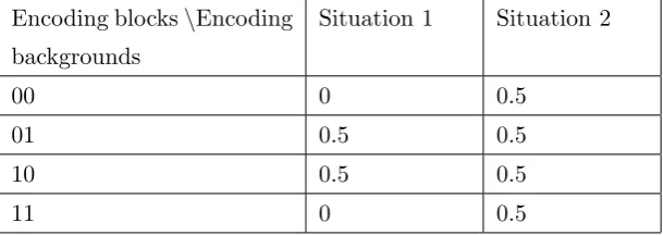
In the following, we will take the (2,2)-MPEM for example to illustrate the parameters in Equation (1). Suppose the currently-processing block is “01” and its encoding background is
Situation 2. We consider its corresponding block on a single share, then p0 = 14, b0 = 0; p1 = 12, b1 = 1; p2 = 41, b2 = 2. It is convenient to know that µ = 1, and σ = 12 = 0.5, which corresponds to the entry of row “01” and column “Situation 2” from Table 1. Due to the symmetry property of shares of the (2,2)-MPEM, the variances of the corresponding blocks on different shares are the same. All possible cases can be found in Table 1.
Encoding blocks\Encoding backgrounds
Situation 1 Situation 2
00 0 0.5
01 0.5 0.5
10 0.5 0.5
11 0 0.5
Table 1: All possible variances of the Hamming weights of an encoding block on a single share.
3.2 Experimental and statistical analysis of the shares encoded by the
(2,2)-MPEM
In this section, we will first give some experimental results for the (2,2)-MPEM. Then we will give some statistical analysis of its share images and explain its security defect.
We use the (2,2)-MPEM to encode image “Pythagoras” and image “Airplane”. The experi-mental results can be found in Figures 1 and 3. Images in Figure 2 are the experiexperi-mental results for the (2,2)-SIVCS proposed by Ito et al. in [10] and Yang in [13].
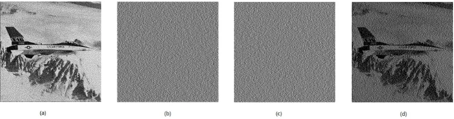
Figure 1: Experimental results for (2,2)-MPEM: (a) the original secret image with image size 340×340, (b) share 1 with image size 340×340, (c) share 2 with image size 340×340, (d) stacked image with image size 340×340
Figure 2: Experimental results for (2,2)-SIVCS: (a) the original secret image with image size 340×340, (b) share 1 with image size 340×340, (c) share 2 with image size 340×340, (d) stacked image with image size 340×340
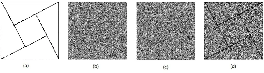
By comparing images (d) in Figures 1 and 2, we can see that the recovered image of the (2,2)-MPEM has better visual quality than that of the (2,2)-SIVCS. However, from images (b) and (c) in Figure 1, we can perceive the content of image (a). Hence we claim that although the MPEM proposed in [5] improves the visual quality of SIVCS, it has security defect on shares. However, for image with complex contours (see image (a) in Figure 3), the shares generated by the (2,2)-MPEM look like noise images (see images (b) and (c) in Figure 3) and provide no information about the secret.
Figure 3: Experimental results for (2,2)-MPEM: (a) the original secret image with image size 512×512, (b) share 1 with image size 512×512, (c) share 2 with image size 512×512, (d) stacked image with image size 512×512
encoded from image “Pythagoras” and those from image “Airplane”, and try to explain why shares of image “Pythagoras” leak the secret while shares of image “Airplane” do not.
Some statistical information of image (a) in Figure 1 can be found in Table 2.
The number of “00” blocks
The number of “01” blocks
The number of “10” blocks
The number of “11” blocks
The total num-ber of blocks
53195 614 1003 2988 57800
Table 2: The numbers of all possible encoding blocks for image (a) in Figure 1
It should be noted that the above statistical information is related to the encoding process. And we encode the original secret image line by line, from left to right, two successive pixels as an encoding block.
Some statistical information of the encoding process of image (a) in Figure 1 can be found in Table 3.
Encoding blocks\Encoding backgrounds
Situation 1 Situation 2
00 28138 25057
01 272 342
10 537 466
11 1539 1449
Table 3: The numbers of all possible encoding blocks which are encoded with all possible encoding backgrounds for image (a) in Figure 1
From Tables 1 and 3, we have the following results:
If the encoding block is “00”, then in overall, the expected variance of the corresponding block on a single share is 2813853195×0 +2505753195×12 = 0.23552.
If the encoding block is “10”, then in overall, the expected variance of the corresponding block on a single share is 1003537 ×12 +1003466 ×12 = 0.5.
If the encoding block is “11”, then in overall, the expected variance of the corresponding block on a single share is 15392988 ×0 +14492988 ×12 = 0.24247.
As we have mentioned, encoding blocks “01” and “10” correspond to contour areas of the secret image, and encoding blocks “00” and “11” correspond to white and black areas of the secret image respectively. Combined with the above calculation, it is convenient to see that from a single share, the expected variance of the contour areas is significantly larger than that of the white and black areas. Besides the contour of image “Pythagoras” is simple, see image (c) in Figure 4. From images (b) and (c) in Figure 1, we can see that the contour areas are more uneven than the black and white areas, which leads us to perceive the content of the secret image. The theoretical analysis agrees well with the experimental result. However, Table 1 in Section 5 of [5] shows that the standard deviations σb and σw defined in Section 5 of [5] are
both 0, which does not agree with the experimental result. Hence we claim that the definition of standard deviation in [5] is improper.
In the following, we will try to explain why the shares of image “Airplane” look like noise images.
Some statistical information of image (a) in Figure 3 can be found in Table 4.
The number of “00” blocks
The number of “01” blocks
The number of “10” blocks
The number of “11” blocks
The total num-ber of blocks
44242 34518 35318 16994 131072
Table 4: The numbers of all possible encoding blocks for image (a) in Figure 3
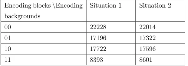
Some statistical information of the encoding process of image (a) in Figure 3 can be found in Table 5.
Encoding blocks\Encoding backgrounds
Situation 1 Situation 2
00 22228 22014
01 17196 17322
10 17722 17596
11 8393 8601
Table 5: The numbers of all possible encoding blocks which are encoded with all possible encoding backgrounds for image (a) in Figure 3
From Tables 1 and 5, we have the following results:
If the encoding block is “00”, then in overall, the expected variance of the corresponding block on a single share is 2222844242×0 +2201444242×12 = 0.24879.
If the encoding block is “10”, then in overall, the expected variance of the corresponding block on a single share is 1772235318× 12+1759635318 ×12 = 0.5.
If the encoding block is “11”, then in overall, the expected variance of the corresponding block on a single share is 169948393 ×0 +169948601 ×12 = 0.25036.
From the above calculation, it is convenient to see that for a single share, the expected variance of the contour areas is significantly larger than that of the white and black areas. However, the contour of image “Airplane” is very complex, where the edge areas and the white and black areas often mix together, see image (d) in Figure 4, leading the shares to look like noise images, see images (b) and (c) in Figure 3. Our experimental result for image “Airplane” agrees well with that of Hou et al. in [5]. That was the very reason that Hou et al. did not notice the security defect on shares.
We use the MATLAB command, “edge(f,‘sobel’,0.15)”, to extract the contour of image “Pythagoras” and image “Airplane”. The experimental result can be found in Figure 4. Image “Airplane” is a halftone image, thus its contour image is very complex.
Figure 4: Edge extraction: (a) image “Pythagoras” with image size 340×340, (b) image “Air-plane” with image size 512×512, (c) contour image of “Pythagoras” with image size 340×340, (d) contour image of “Airplane” with image size 512×512
4
Using average contrast and variance to evaluate the visual
quality of VCS
Contrast is first introduced in the pioneer work of Naor and Shamir to evaluate the visual quality of VCS. However, researchers do not reach a consensus on the definition of contrast. There are four definitions of contrast: αN S = hm−l introduced in [9], αV V = mh(h−+ll) introduced
in [12],αES = mh−+ll introduced in [4] andαLW L = h(m−h()+h−l(lm)m−l)+m2 introduced in [8].
Unfortu-nately, they are all inappropriate to reflect the overall contrast and the gray-level variation of the recovered image, because of the following reasons:
block of a white pixel, there might be the case thath andl occur with very small probabilities and thus cannot reflect the overall gray-level of the recovered block of black and white pixels respectively, see Schemes 3 and 4.
Reason 2: All the above definitions of contrast do not consider the variance of all possible Hamming weights of the recovered block of black and white pixels. However, as we will show later, variance not only effects the visual quality of SIVCS, see [5] and [7], but also effects the visual quality of VCS, see Schemes 1 and 2.
Schemes 1−4 are all (2,2)-VCSs with pixel expansion 4. M0= [
01 01
]
andM1 = [
01 10
] .
Scheme 1: If the pixel to be shared is white (resp. black), we randomly permute the columns of M0 (resp. M1), and distribute two sub-pixels for each share. Then, we pick up a column fromM0 (resp. M1), and distribute one sub-pixel for each share. For the second time, we pick up a column from M0 (resp. M1), and distribute one sub-pixel for each share.
Scheme 2: If the pixel to be shared is white (resp. black), we randomly permute the columns of M0 (resp. M1), and distribute two sub-pixels for each share. Repeat the above process for two times.
Scheme 3: If the pixel to be shared is white, we randomly permute the columns ofM0 and distribute two sub-pixels for each share. Then we choose M1 with probability 1001 and choose M0 with probability 10099 and randomly permute the columns of the chosen basis matrix Mi and
distribute two sub-pixels for each share. If the pixel to be shared is black, we randomly permute the columns ofM1 and distribute two sub-pixels for each share. Then for the second time, we randomly permute the columns ofM1 and distribute two sub-pixels for each share.
Scheme 4: If the pixel to be shared is white, we randomly permute the columns ofM0 and distribute two sub-pixels for each share. Then we choose M1 with probability 10099 and choose M0 with probability 1001 and randomly permute the columns of the chosen basis matrix Mi and
distribute two sub-pixels for each share. If the pixel to be shared is black, we randomly permute the columns ofM1 and distribute two sub-pixels for each share. Then for the second time, we randomly permute the columns ofM1 and distribute two sub-pixels for each share.
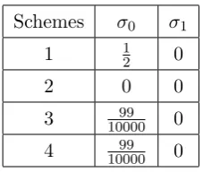
We use the variance defined in Equation (1) to measure the gray-level variation of the recovered image. σ0 denotes the variance for sharing a white pixel andσ1 denotes the variance for sharing a black pixel. The variances of Schemes 1−4 can be found in Table 6. The contrasts and average contrast ¯α of Schemes 1−4 can be found in Table 7.
Schemes σ0 σ1
1 12 0
2 0 0
3 1000099 0 4 1000099 0
Schemes αN S αV V αES αLW L α¯
1 13 201 15 194 12 2 12 101 25 45 12 3 13 201 15 194 199400 4 13 201 15 194 101400
Table 7: The contrasts and average contrast of Schemes 1−4.
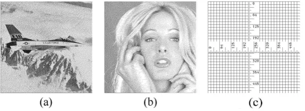
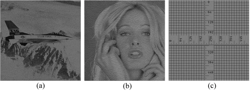
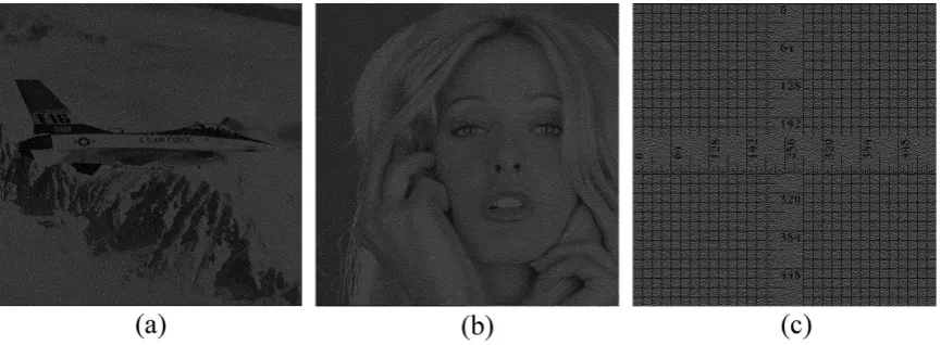
The three secret images are (a−c) in Figure 5. The visual quality of Schemes 1−4 can be found Figures 6−9 respectively.
As Schemes 1 and 2 are of the same average contrast, according to Table 6 and Figures 6−7, it is easy to see that smaller variance will result in better visual quality. From the perspective of contrastαN S orαV V orαES orαLW L, and according to Table 7, we can see that Schemes 1,
3 and 4 should have almost the same visual quality, which does not agree with the experimental results, see Figures 6, 8 and 9. Even if we combine contrastαN S orαV V orαES orαLW L with
variance, according to Tables 6 and 7, we can see that Schemes 3 and 4 should have almost the same visual quality, which also does not agree with the experimental results, see Figures 8 and 9. However, average contrast ¯α reflects the differences between Scheme 3 and Scheme 4, which agrees well with the experimental results, see Figures 8 and 9. Although from the perspective of contrast αN S or αV V or αES or αLW L, Scheme 2 is significantly better than Scheme 3,
their visual qualities are very close, see Figures 7 and 8, which on the other hand agrees well with average contrast ¯α. Hence we claim that only the combination of average contrast ¯α and variance can correctly reflect the experimental results.
Figure 5: The original four secret images: (a) air plane, (b) face, (c) ruler. All are of image size 512×512
5
Conclusions
Figure 6: The experimental results for Scheme 1. All are of image size 1024×1024
Figure 7: The experimental results for Scheme 2. All are of image size 1024×1024
Figure 9: The experimental results for Scheme 4. All are of image size 1024×1024
evaluate the visual quality of VCS.
References
[1] G. Ateniese, C. Blundo, A. De Santis, and D.R. Stinson. Visual cryptography for general access structures. InInformation and Computation, volume 129, pages 86–106, 1996.
[2] M. Bose and R. Mukerjee. Optimal (k, n) visual cryptographic schemes for general k. In
Designs, Codes and Cryptography, volume 55, pages 19–35, 2010.
[3] S. Droste. New results on visual cryptography. In CRYPTO ’96, Springer-Verlag Berlin LNCS, volume 1109, pages 401–415, 1996.
[4] P.A. Eisen and D.R. Stinson. Threshold visual cryptography schemes with specified white-ness levels of reconstructed pixels. InDesigns, Codes and Cryptography, volume 25, pages 15–61, 2002.
[5] Y.C. Hou and S.F. Tu. A visual cryptographic technique for chromatic images using multi-pixel encoding method. In Journal of Research and Practice in Information Technology, volume 37, pages 179–191, 2005.
[6] I.K. Kang, G.R. Arce, and H.K. Lee. Color extended visual cryptography using error diffusion. In IEEE Transactions on Image Processing, volume 20, NO.1, pages 132–145, 2011.
[7] F. Liu, T. Guo, C.K. Wu, and L. Qian. Improving the visual quality of size invariant visual cryptography scheme. InJ. Vis. Commun. Image R., volume 23, pages 331–342, 2012.
[9] M. Naor and A. Shamir. Visual cryptography. In EUROCRYPT ’94, Springer-Verlag Berlin, volume LNCS 950, pages 1–12, 1995.
[10] Ito. R, Kuwakado. H, and Tanaka. H. Image size invariant visual cryptography. InIEICE Transactions on Fundamentals of Electronics, Communications and Computer Science, volume E82-A.No.10, pages 2172–2177, 1999.
[11] S.J. Shyu and M.C. Chen. Optimum pixel expansions for threshold visual secret sharing schemes. InIEEE Transactions on Information Forensics and Security, volume 6, NO.3, pages 960–969, 2011.
[12] E. Verheul and H.V. Tilborg. Constructions and properties of k out of n visual secret sharing schemes. In Designs Codes and Cryptography, volume 11, No.2, pages 179–196, 1997.