Article
A Density-Based Clustering Method for Urban Scene
Mobile Laser Scanning Data Segmentation
You Li 1, Lin Li 1,2,3, *, Dalin Li 1, Fan Yang 1, and Yu Liu 1
1 School of Resource and Environment Sciences, Wuhan University, 129 Luoyu Road, Wuhan 430079, China; [email protected]
2 Collaborative Innovation Centre of Geospatial Technology, Wuhan University, 129 Luoyu Road, Wuhan 430079, China; [email protected]
3 The Key Laboratory of GIS, Ministry of Education, China, Wuhan University, 129 Luoyu Road, Wuhan 430079, China; [email protected]
* Correspondence: [email protected]; Tel.: +86-027-68778879
Abstract: The segmentation of urban scene mobile laser scanning (MLS) data into meaningful street objects is a great challenge due to the scene complexity of street environments, especially in the vicinity of street objects such as poles and trees. This paper proposes a three-stage method for the segmentation of urban MLS data at the object level. The original unorganized point cloud is first voxelized, and all information needed is stored in the voxels. These voxels are then classified as ground and non-ground voxels. In the second stage, the whole scene is segmented into clusters by applying a density-based clustering method based on two key parameters: local density and minimum distance. In the third stage, a merging step and a re-assignment processing step are applied to address the over-segmentation problem and noise points, respectively. We tested the effectiveness of the proposed methods on two urban MLS datasets. The overall accuracies of the segmentation results for the two test sites are 98.3% and 97%, thereby validating the effectiveness of the proposed method.
Keywords: mobile laser scanning; voxel; clustering; segmentation
1. Introduction
With the developing ability to acquire high-quality point cloud data, mobile laser scanning systems have been widely utilized for various applications such as 3D city modeling [1], road inventory studies [2], safety control [3], car navigation [4], and forestry management [5]. Data from mobile laser scanning (MLS) systems, airborne laser scanning (ALS) systems and terrestrial laser scanning (TLS) systems are being widely applied in urban scene analysis. However, MLS data are more suitable for urban scene information extraction for two reasons. First, compared to ALS data, MLS data are of higher density and contain more vertical information, factors that are of great importance in identifying detailed information from poles and buildings. Moreover, MLS data are more efficiently acquired than TLS data, as the latter are collected by manually positioned systems. Many researchers have studied the use of MLS data in urban scenes intensively, including in road [6,7] and road marking [8-10] detection, building detection and reconstruction [11-13], pole-like object detection [3,14,15], tree detection and modeling [16-18], and urban scene segmentation and classification [19-23].
data volume. Second, the purpose of segmentation is to find some universal criterion to segment MLS point cloud into discrete objects, although the objects often have different sizes and shapes. The last challenge is derived from the scene complexity of urban environments, where cars remain close to each other, trees and pole-like objects are tangled with each other and various objects can lie under trees and poles.
The segmentation of ALS data has been intensively studied in the past decade [1,22,25]. However, methods for the segmentation of ALS data are only partially applicable for MLS data due to differences in point densities, scanning patterns, and geometric characteristics [20]. Recently, to overcome the above-mentioned challenges, several methods have been proposed to segment MLS data. Most of these researchers have made great contributions to this area and could segment MLS data with high precision in many different scenes of urban areas. However, their methods still need further improvement to overcome under- and over-segmentation problems in complex scenes where objects are tangled with each other or where a huge variety of point density exists.
We proposed a method that can effectively segment MLS point clouds in a complex scene with tangled objects and large data density variations. This paper is organized as follows. Related work on MLS data segmentation is presented in Section 2. The proposed method is described in detail in Section 3. The results of two experiments on urban scenes and some comments of them are presented in Section 4. The conclusions about the advantages and disadvantages of the proposed method and future work in our research are discussed in Section 5.
2. Related works
Most previous works have focused on discussing the methods used to segment MLS data, and little attention has been paid to hidden cues to discriminate different objects. The cues utilized in existing methods can be categorized into three classes: Euclidean distance, geometric features and other features, including intensity and color features.
2.1. Euclidean Distance
In some relatively simple situations where there exists distinguishable space between objects, the Euclidean distance cue alone is sufficient to differentiate street objects. The traditional connected component analysis method only needs to utilize a fixed radius for segmentation. The most common workflow for these methods is to first detect ground surface and remove these corresponding points from the dataset; then, connected component analysis is applied for the remaining point set to segment objects [22]. Pu, Rutzinger, Vosselman and Oude Elberink [3] utilized a similar workflow to recognize basic structures from mobile laser scanning data for road inventory studies. Their method first partitioned the whole point cloud dataset to strips along the road directions in the pre-processing stage. Then, the whole dataset was classified into ground, off-ground and on-ground points. After removing the off-ground and ground points, the remaining on-ground points were segmented and assigned unique IDs by performing connected component analysis using the Euclidian cue. Then, a single class of objects was recognized using numerous other features of the segments. Similarly, Oude Elberink and Kemboi [26] also utilized the distance cue to distinguish objects with the connected components analysis method. However, this method could address more complicated situations because it introduced a new technique to re-segment mixed trees.
showed that their improved method was better than the connected component analysis method with the fixed radius configuration.
Other scholars have incorporated an auxiliary density with the Euclidian distance cue to segment point clouds. For example, El-Halawanya and Lichtia [28] first filtered out ground points based on density and then, based on the assumption that the distance between pole-like objects was greater than 1 meter, segmented the remaining data using a vertical region growing method. Golovinskiy, et al. [29] also utilized the Euclidian distance property with density to segment objects in urban areas. This paper proposed a four-stage workflow to segment and classify urban scene point cloud data, namely, through localization, segmentation, feature extraction and classification. The graph cut method, which is broadly used in image segmentation, is applied in the third stage. In this graph-cut-based segmentation method, objects with large distances and few points between borders were assumed to be weakly connected and were thus segmented.
Methods mainly based on the Euclidian distance cue represent quick and simple methods of segmenting point clouds because no local-neighborhood-based feature calculation is needed. However, these methods are only robust when there is a discernible distance between objects in simple situations. Furthermore, for methods based on the density cue, a global density threshold is needed to differentiate objects. Therefore, these methods are not robust for scenes with large density varieties, which is a common situation in large mobile laser scanning datasets.
2.2. Geometric features
Due to the presence of noise data and the variety of object sizes and shapes, a segmentation method using a single cue is not sufficient. To differentiate more accurately street furniture, other cues are needed besides Euclidian distance. The most frequently used cues for discriminating street objects are local-neighborhood-based geometric features, including normal vector, smoothness, roughness, major direction and dimensionality.
The normal vector cue is effective in segmenting planar street elements, such as buildings and ground planes, from the other objects. Vosselman, et al. [30] focused on the detection of surfaces from point clouds and believed that the recognition of surfaces can be regarded as a point cloud segmentation problem. Smooth surfaces were often extracted by grouping nearby points that share the same property such as the direction of a locally estimated surface normal. The proximity of points (Euclidian distance), local planarity and smooth normal vector field were considered as criteria for growing of surfaces in region growing methods. Attention has also been paid to segmenting buildings into different planes based on normal vectors [11,13]. Vo, Truong-Hong, Laefer and Bertolotto [13] presented the drawbacks of three types of time-consuming segmentation methods and increased the speed of segmentation by introducing a new octree-based method. After voxelization and saliency estimation, the actual segmentation could be roughly divided into two separate steps. The first step was to roughly cluster points from the same surface using region growing based on the normal vector cue. Then, a refining stage was applied to re-process those points that were on boundaries and un-reached points. The normal vector cue also served as an important role in merging segments in segment-based method [19]. The whole scene was partitioned into individual grids to detect ground using RANSAC. Then, the Euclidian distance was utilized as the only feature to form super-segments in the first segmentation stage. Finally, the normal vector was used to judge if neighboring super-segments could be merged.
pole-like objects in urban point cloud data. In this method, a geometric parameter called the Geometric Index (GI) was employed to segment ground and buildings from the point clouds. The normal vector and roughness values of every point were important elements of the GI. Roads were considered as having low GI values, while facades had high GI values.
Moreover, other geometric features, such as major direction and dimensionality, have been applied in other research to discriminate different objects in point cloud data. Prior to Demantké, et al. [33], geometric features based on local neighborhoods were all computed by counting a fixed number of points around every point or counting the number of points within a fixed radius, both of which were considered to be inaccurate for point clouds with uneven densities. This research therefore proposed a new method to calculate the dimensionality of every point based on optimal radius using the entropy function. The local shape of every point was calculated as linear, planar, or volumetric through a combination of the eigenvalues of the local structure tensor. Adjacent points with the same dimensionality were clustered together. Based on this method, Yang and Zhen [20] introduced a new shape-based segmentation method for mobile laser scanning data. In this method, many geometric features, including the normal vector, major direction, and dimensionality, were incorporated in the segmentation in different stages; the experimental results were reported to be better than those of most previous studies.
Geometric-feature-cue based methods are better than pure-distance-based methods on complex scenes in terms of accuracy because more clues of differences between objects are incorporated. However, they are more time consuming due to the heavy computational load resulting from the geometric feature calculation for every point. Moreover, calculating geometric features accurately in tangled situations of urban scenes remains a challenge even though the optimal-radius-based method is used. This is because, in such situations, the geometric features of points at borders of objects are difficult to compute accurately, while these points are sometimes crucial in segmenting tangled objects.
2.3. Other features
In addition to distance and geometric features, intensity and color are also widely used cues in the segmentation of point clouds. Segmenting point clouds using multiple cues and integrating variable data sources should provide richer descriptive information and have better prospects for obtaining good results. Intensity values can reveal the material information of targeted objects to some extent, while color values can provide information about the state of a target object in addition to material information.
Intensity has been a widely utilized cue in the segmentation of road markings and road signs [8-10,34-37]. Intensity values are crucial in these methods because road markings are usually made of special pavement marking material and have higher reflective ability than does the remainder of the road surface. A traditional method for the segmentation of road markings is to project the point cloud onto the horizontal plane to build feature images and perform segmentation on these images using image segmentation methods. Chen, Kohlmeyer, Stroila, Alwar, Wang and Bach [37] proposed a similar method to extract road signs and reconstruct road markings. To extract road signs, the original data were first filtered based on the distance to the sensor, sensor angle and intensity. After clustering using connected component analysis, road sign planes were fitted using the RANSAC algorithm. To extract road markings, roads were first extracted by identifying road boundaries, including raised curbs and barriers and border lines. Then, the intensity values of points were used to select possible road marking points. After the feature images were generated, road markings in the image were detected using image processing techniques. Three-dimensional road markings were obtained by back-projecting the image to the original point clouds. To summarize, intensity values were of great importance both in road sign detection and road marking extraction. Aside from road markings and road signs, intensity values also played an important role in detecting cracks on roads using mobile laser scanning data [38].
incorporating point intensity, more accurate shape estimations were obtained. Intensity, along with the principle direction and normal vector, also played an important role in the later process of merging points with identical labels, which segmented points of the same dimensionality. Barnea and Filin [24] integrated color image data into the segmentation of terrestrial laser scanning data. The integration of geometric information and color image information provided greater potential for later processing. Yang, Dong, Zhao and Dai [21] applied almost all the above-mentioned cues in their newly published research, including distance, normal vector, major direction, dimensionality, intensity and color. Color and intensity were utilized to transform neighboring homogeneous points into super-voxels in the first stage of their method. Then, the method applied a graph cut algorithm that covered various cues, including intensity, normal vector, major direction and distance, to segment three type of super-voxels. Finally, these segments were merged based on pre-defined sematic information according to their saliency values. With so many cues incorporated in the proposed method, the experimental results showed that the detection accuracy was better than that of most previous studies.
Despite the fact that objects become more differentiable when incorporating auxiliary cues, such as intensity and color information, the additional information results in more computation time and is not always accessible.
Generally speaking, current methods based on the above-mentioned cues for street furniture segmentation can perform well in many situations. However, these methods need further improvement for use on complex scenes from two aspects. First, a new definition of density is needed to address data with large density variations. Second, new segmentation cues to differentiate close and tangled objects are needed. To obtain better results, a density-based clustering method that introduces two new cues (local density and minimum distance) is presented in this paper for the segmentation of urban MLS point clouds.
3. Methods
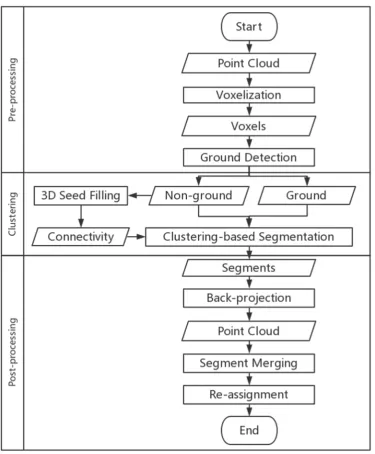
The proposed method attempts to segment MLS data from urban scenes into discernible and meaningful segments that can be applied for further street furniture extraction and classification. The method consists of three main phrases (Figure 1):
1. Pre-processing: Original un-organized MLS data are cleaned and re-organized based on voxels; then, the whole scene is classified into ground and non-ground voxels.
2. Clustering: A density-based clustering method is utilized to segment the non-ground voxels into discrete clusters.
Figure 1. The overall workflow of the proposed method.
3.1. Pre-processing
This phrase attempts to provide clean and organized data for the following clustering algorithm, including voxelization of points into voxels and detection of ground voxels. Due to the complexity of scanning environments in urban scenes, noise points that are isolated from the remaining point cloud are brought into the original MLS data. These noise points negatively affect the following algorithm; thus, they need to be detected and removed from the original MLS data. Isolated points are detected and removed using the connected component analysis method, and small clusters are considered as noise points and filtered out from the original MLS data.
3.1.1. Voxelization
re-organizes and condenses the original data into a 3D space. In this context, a voxel is a cube that records three classes of information: voxel location, voxel index and number of points in the voxel. A voxel location is represented by three numbers , , , which represent the location of the voxel relative to the minimum x, y, and z position of the original point cloud. The location of the voxel can be computed using the following equation:
= ( − ) (1)
where denotes the minimum x of all points in the point cloud and is the voxel size. and are calculated in a similar way.
After the processing step of the voxelization, all needed information for steps before the merging processing step are stored in the voxels, and all steps before merging are applied to the voxel set.
3.1.2. Ground detection
A whole urban scene point cloud can be roughly classified into off-ground points, on-ground points and ground points [3]. Segmentation targets in this paper are street furniture that stands on or close to the ground. To select these targets, the ground voxels need to first be detected. Numerous researchers have focused their effort on the detection or even reconstruction of roads from point cloud data [2,6-10,34-36]. In addition, roads can sometimes play the role of ground to provide the relative position of street furniture to the ground in situations where the ground is mainly even vertically along the trajectory. Nevertheless, in this context, complex situations of wide and uneven streets are considered. Moreover, in our next processing step for calculating parameters of the clustering algorithm, the objects’ distances to the ground rather than to the road need to be calculated. Therefore, we introduced a new ground detection method applied to the voxel set generated in the previous step.
Ground is assumed to be relatively low in a local area and erected low vertically compared to on-ground objects. Therefore, ground can be separated from the whole scene by analyzing the relative height and the vertically continuous height ( ) of each horizontally lowest voxel (HLV) in the whole voxel set. The height of a voxel is represented by , as depicted in Eq. (1). Voxels that satisfy the conditions in Eq. (2) are recognized as ground voxels:
< 1/ && < 0.5/ (2)
where is the vertically continuous height of an HLV, is the relative height of an HLV to the lowest voxel in its neighborhood, and is the voxel size. The vertical continuity analysis algorithm for calculating is depicted in detail in a previous study (Li et al., 2016). Utilizing the proposed algorithm, curbs and low-elevation bushes are also classified as ground and are thus filtered out before clustering.
3.2. Clustering
After ground voxels are detected from the original voxel set, the remaining voxels need to be segmented for further extraction or classification of street objects. To this end, we proposed a clustering-based method for segmentation. Inspired by the algorithm implementing clustering via fast search and finding density peaks [39], we also make two assumptions about cluster centers: (1) the center of a cluster is surrounded by voxels with lower local densities, and (2) the cluster centers are relatively far away from other cluster centers compared to its local neighboring voxels. Detailed information about the clustering method is descripted in the two sections below.
3.2.1. Generation of cluster centers
definition of cluster centers, and δ , which represent the local density parameter and the minimum distance parameter of a voxel .
Local density: The local density parameter mainly indicates the vertically continuous height of a voxel at one horizontal location ( , ), and it is also affected by two other factors: the vertical position of the voxel ℎ, and the number of points in the voxel . For every voxel , the density parameter can be formulated as
= − + , <
( − + ) , ≥ (3)
where depicts voxel ’s vertical distance to the ground specified by Eq. (4). In Eq. (4), is the horizontally closest voxel to in the ground voxel set. is a threshold value based on real situations, and denotes the maximum number of points in one voxel.
= − (4)
Minimum distance: The minimum distance parameter δ indicates the distance between the current voxel and the closest voxel that has a higher density as specified by Eq. (3). indicates a customized distance between voxels and . The distance can be calculated according to Eq. (5) as follows:
= , =
, ≠ (5)
where indicates the label of voxel specified by the three-dimensional seed filling algorithm, indicates the radius for searching neighbors, and is the Euclidian distance between voxels and .
For every voxel , the distance parameter δ can be measured by the following formula:
{ }
=
≠
=
∈Φ
I
D
Φ
I
,
d
δ
i S neighbor i S I j iji Si
,
min
(6)
where is a voxel set, whose elements have a higher density than voxel and lie within a neighbor distance to voxel . can be measured by the following formula:
= ∈ : > && < (7)
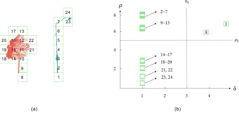
Cluster center: After the local density parameter and minimum distance parameter for every voxel have been calculated, the cluster centers can be determined. Based on the two above-mentioned assumptions, cluster centers should have both high local density value and minimum distance value. Therefore, voxels with both a higher value than the local density threshold value and minimum distance threshold value δ are considered to be cluster centers. Cluster centers in the proposed method have practical meaning; they normally depict the highest part of street objects. The local density parameter generally indicates the height of an object, and the minimum distance parameter indicates the distance between two objects in certain ways. Assume that C= represents the label of each voxel and that = represents the index of the cluster centers. The label of each voxel is determined based on the formula below:
= ,−1,∈ ( =∉ ) (8)
local densities. From the figure, it can be concluded that the two cluster centers at the bottom part of two street objects can easily be found, as they have both high local density and minimum distance values.
Figure 2. An example of selecting cluster centers: (a) voxels numbered by descending local density values; (b) local density and minimum distance values distribution of the voxels from (a).
3.2.2. Clustering
Based on the assumptions about cluster centers, they can be determined by choosing voxels that have both higher local density and minimum distance values. Then, the label of each voxel can be obtained in the sequence of local densities in descending order. Every non-center voxel’s label is determined by the neighboring voxel, which is the closest voxel having a higher local density than the current voxel within a neighboring distance. Assume that the voxel set sorted with the local density by descending order is . The neighboring voxel index of each voxel v can be specified by the following formula:
{
}
=
=
≠
>
=
< neighbor i neighbor i m m i j mD
δ
i
D
δ
i
d
n
i ij
||
1
0,
&
&
1
,
argmin
(9)where δ is the minimum distance parameter defined in Eq. (6).
When the neighbor voxel of each voxel in the voxel set is configured, the clustering procedure is performed based on the sequence of local densities in descending order, as described in detail in Algorithm 1.
Algorithm 1: Clustering Input:
: voxel set for clustering Parameters:
N: total amount of voxel
: radius for searching closest neighbors Start:
(1) Calculate R= based on Eq. (3).
(2) Sort R by descending order SR= .
(3) Calculate D= from Eq. (6).
(5) Initialize the label of each voxel from Eq. (8).
(6) for each voxel in SR repeat:
(7) if = −1:
(8) =
End
Output:
C:cluster labels of
After the clustering of the voxel set, most narrowly expanded objects, such as most trees, light poles and cars, are well segmented. However, some widely expanded objects are over-segmented, which requires further processing. Moreover, based on the clustering algorithm, some voxels that have high minimum distance values but low local density values are not labeled. These voxels are regarded as halo voxels and need to be processed in the following re-assignment step.
3.3. Post-processing
Once the clustering processing step is completed, the whole voxel set is segmented into clusters with different labels. However, the size of the cluster is constrained to a fixed size around the cluster center due to the limitation of radius in finding neighboring voxels, which leads to over-segmentation and halo voxel problems for large street objects. Therefore, further post-processing steps are needed to address these problems. First, a merging step applied to the back-projected point cloud is used to merge clusters of large objects. Then, we present a re-assignment processing step to address those halo voxels generated in the previous clustering stage, in which some of these voxels are filtered out and others are merged with nearest segments.
3.3.1. Merging of clusters
Most trees and pole-like objects are often differentiable after the clustering stage because the pole-part of these objects can always play the role of a cluster center and because the spaces between different pole-parts are recognizable. However, large street objects are often over-segmented into various parts. Consequently, a merging step is introduced in this method to address the over-segmentation problem. To improve the accuracy, the voxels are first back-projected to points. The following processing steps, including the merging and refinement step, are both applied to the point cloud instead of the voxel set. As presented in the voxelization step, a one-to-one correspondence is built between each point and each voxel; hence, we can obtain a point cloud with corresponding labels through the voxel index stored at each point and each voxel.
In the merging step, a new merging algorithm is incorporated to merge neighboring clusters via region growing. The merging criteria are the connectivity and the curvature similarity of two clusters at their common borders. The connectivity of two clusters and is measured by the distance between them, which is the distance between the closest points in two clusters defined by the following formula:
= , (10)
where and represent points in clusters and , respectively, and , denotes the Euclidean distance between two points. and can be recognized as neighboring clusters (NCs) only when is smaller than the threshold value of 0.5 meters.
have two points from two NCs, and the distance between them is lower than a threshold value. Assume that and are two NCs. The contained pair point set (PPS) can be defined as follows:
= , : , < , ∈ , ∈ (11)
where is a point in and is a point in . When the distance between them is less than (0.5 m), , is considered to be an element of the PPS.
The curvature similarity of a point can be measured change rate of normal which can be defined by the following formula:
= (12)
where , and are the eigenvalues of a point in descending order, which is calculated through Principal Component Analysis (PCA). In addition, the curvature similarity of two clusters can be measured as follows:
= 1
2 + (13)
where ( , ) is the pair point element in the pair point set , and , are the
corresponding curvatures of the pair point measured based on Eq. (12). Then, the rules for merging two clusters are as follows:
< && <
where is a threshold value already defined in Eq. (11) and is a threshold value found by analyzing thousands of sample data. The merging processing step traverses all the clusters generated in the previous step and generates new segments that correspond to street furniture at the object level by applying region growing.
3.3.2. Re-assignment
The clustering stage generates halo voxels that have high minimum distance values but low local density values. These voxels often correspond to borders of large trees that are far from the pole part of the tree and extruded parts or other parts of buildings that are not fully scanned by the laser beams. They are all not labeled in the clustering step, and they are also back-projected to points in the merging step. Therefore, we can process these halo points independently after the merging step. All these halo points are clustered using the connected component analysis algorithm, and then, the result clusters are merged with the closest segments generated in the merging step. However, those points that are far away from all segments are regarded as noise points and are filtered out.
4. Experiments
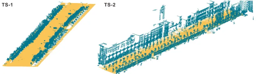
Two test sites from Wuhan city were chosen to test the effectiveness of our method. Test site 1 (TS-1) was acquired in the suburb area of Wuhan city, which has tangled street trees and poles in wide streets with high density variations. Test site 2 (TS-2) was located at Optical Valley, with substantially more street object categories; Optical Valley is a typical urban area in Wuhan City. Detailed information about the two test sites can be found in Table 1.
Table 1. Description of the test sites.
Test Sites Length(m) Average Width(m) Points(million) Density(points/m2)
TS-1 303 60 6.8 374
TS-2 285 30 2 234
According to the proposed method, the voxel size should be decided first prior to performing voxelization and then ground detection. The density of mobile laser scanning data in each test site varies substantially both in between the test sites and at each test site. The voxel size should be configured based on the overall consideration of the above-mentioned criterion, the density of the test site and the following voxel continuity judgment step of objects that are far away from the trajectory. The average point span for distant objects in the test sites is greater than approximately 0.15 m. To guarantee that distant objects have vertically continuous voxels, the voxel size was configured as two times the average point span: 0.3 m. The numbers of voxels after the voxelization of TS-1 and TS-3 are 170,864 and 157,674, respectively, with compression rates (1 - number of voxels containing data / number of original points) of 97.5% and 92.1%. After voxelization, the ground can be detected based on Eq. (2). The results for each test site after back-projection from voxels to points are presented in Figure 3, where the orange points are ground points.
Figure 3. Ground detection results after back-projecting to point clouds.
4.2. Clustering results
After filtering out ground voxels, the clustering-based segmentation processing step is then applied to the remaining voxel set, which produces cluster centers and subsequently segments from these cluster centers. The cluster centers are determined based on two key parameters, local density and minimum distance, which are defined in Eq. (3) and Eq. (6) in Section Error! Reference source not found.. The parameter configuration for the generation of cluster centers can be found in Table 2.
Table 2. Parameters configurations.
Parameters Values Number of Voxels
1.2m 4 0.9m 3 1.5m 5 3.9m 13
not over-segmented, which results in greater merging and re-assignment work during the post-processing step.
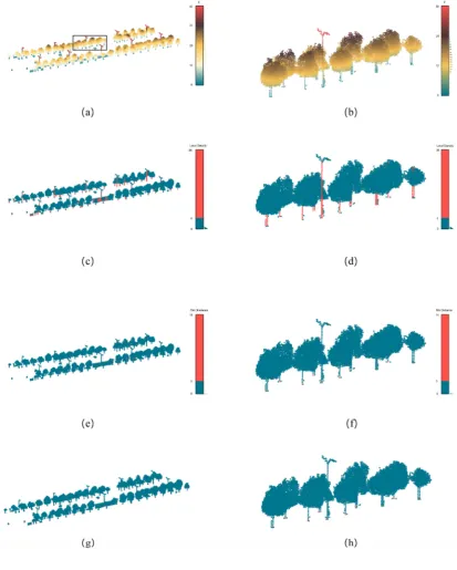
The cluster center generation results for a typical scene are presented in Figure 4. A point in the figure corresponds to a voxel and is located at the center of the voxel. The cluster center generation results of the selected part of the test area are depicted in red in Figure 4(h). From this figure, it can be concluded that all street objects can be located based on the cluster centers labeled in the figure.
Figure 4. Cluster centers generation results in a typical scene: (a) original voxel set colored by Z coordinate; (b) selected voxel set in black rectangle from (a) colored by Z coordinate; (c) local density values distribution of the original voxel set; (d) local density values distribution of the selected voxel set; (e) minimum distance values distribution of the original voxel set; (f) minimum distance values distribution of the selected voxel set; (g) cluster centers (colored in red) generation results of the original voxel set; (h) cluster centers (colored in red) generation results of the selected voxel set.
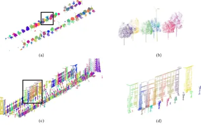
Figure 5. Clustering results after back-projection to points for the test sites: (a) an overall scene from TS-1; (b) typical tangled trees and poles that are well-segmented; (c) the overall scene of TS-2; (d) buildings that are over-segmented.
4.3. Merging and re-assignment results
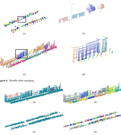
After the merging process, 202 and 380 segments were generated in TS-1 and TS-2, respectively. Figure 6 depicts the results after merging for the two test sites. We can conclude that fences were successfully merged to form meaningful street objects after our merging method was applied. Moreover, some building failed to be merged, as they were only partially reached by the laser beams because of the occlusions caused by the trees in front of them and the large space between the buildings and the laser scanner. However, it is also meaningful to segment buildings to this extent because they can also be detected in the subsequent extraction or classification stage if the overall geometry, such as the width of the segment, is not considered.
Figure 6. Results after merging.
Figure 7. Results of the re-assignment step (red colored points in (a) and (c) represent the halo points that were re-assigned to the (b) and (d) individually)
4.4. Performance analysis of final results
can conclude that these criteria can successfully reveal the quality of the results in a direct manner, as they concentrate on evaluating the results at the object level.
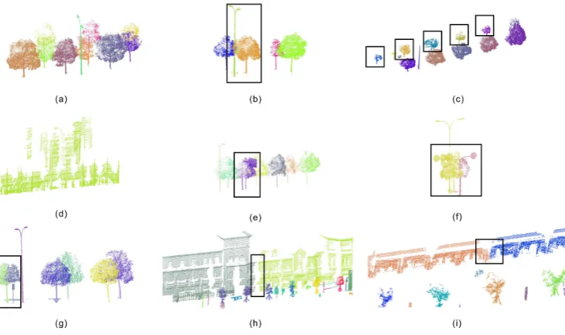
It can be seen that the proposed method can achieve high accuracy in segmenting the data of both test sites (OA of 98.3% and 97%), with tolerable minor errors. First, the method can not only perform well in simple situations with differentiable space between objects but also obtain high accuracy in complex situations where trees and poles are tangled together (Error! Reference source not found.(a), (b)). Second, TS-1 had two lines of trees along the street with large density variations; our method can overcome the uneven density problem in TS-1 and can also segment the trees laying behind with first row of trees and poles with lower density (Figure 8 (c)). Moreover, the method is also robust in terms of addressing buildings with complicated structures in TS-2 (Figure 8 (d)). Although some low density and occluded parts of the building were recognized as noise points at the clustering stage, they are re-assigned to the building successfully at the final stage of the method. The segmentation errors in TS-1 mainly result from under-segmentation problems, mainly caused by the nesting of objects. For example, two under-segmented trees are tangled with traffic signs in TS-1, and the pole parts are nested within each other, which makes it difficult to differentiate them correctly (Figure 8 (e), (f)). One tree was over-segmented because one traffic sign with a low height was laid right down upon it (Figure 8 (g)). Two similar under-segmentation results also existed in TS-2, namely, those present in Figure 8 (e) and (f). One tree was over-segmented for a reason similar to that in Figure 8 (g). The major over-segmentation originates from the buildings in TS-2, where three buildings are over-segmented for two reasons. First, some building segments are far away from the segments in the same building because of the absence of laser beams in certain parts of the segments due to occlusions (Figure 8 (h)). The other source of errors is the irregular distribution of the points at the common border of two over-segmented building parts, which lead to the unsuccessful merging of two segments in one building (Figure 8 (i)). However, most of the buildings in the test sites are well segmented if they are not occluded excessively. In addition, these over-segmentation errors will not inhibit the recognition of these segments as buildings as long as the sizes of these segments are not used as the segment features.
= ℎ ℎ
= ℎ
= 1 − +
2
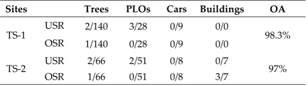
Table 3. Performance analysis for segmentation results of two test sites.
Sites Trees PLOs Cars Buildings OA
TS-1 USR 2/140 3/28 0/9 0/0 98.3%
OSR 1/140 0/28 0/9 0/0
TS-2 USR 2/66 2/51 0/8 0/7 97%
Figure 8. Typical scenes in the test sites.
5. Conclusions
This paper proposes a three-stage density-based clustering approach to segment urban scene MLS data. First, after filtering out noisy points, the original point cloud dataset is voxelized, and the ground voxels are detected based on the assumptions that we make about them. In the second stage, the key clustering processing step is performed. The cluster centers are found based on two key parameters: local density and minimum distance. In addition, the labeling process is performed in descending order of each voxel’s local density value. In the final stage, a merging step is first applied to the back-projected point cloud to merge those segments generated in the second stage. Finally, a re-assignment step for processing the noise points is conducted to produce the final segmentation results. Situations where large density variations exist in mobile laser scanning data are also fully considered in the proposed method. Moreover, the proposed method does not require additional information except for the coordinates of the point clouds. The experimental results show that our method can effectively segment urban mobile laser scanning data in variable cases, with an overall accuracy of greater than 97% based on our proposed criteria. The results also indicate that the proposed method can perform well not only in simple situations where there is discernible space between objects but also in complicated scenes where trees and poles are tangled together. However, as presented in Section 4.4, poles and trees that are too nested with each other cannot be segmented well; this requires further improvement in our future studies.
Acknowledgments: This study is funded by Scientific and Technological Leading Talent Fund of National Administration of Surveying, mapping and geo-information (2014), the Wuhan ‘Yellow Crane Excellence’ (Science and Technology) program (2014) and the Fundamental Research Funds for the Central Universities (2012205020211).
Author Contributions: All authors contributed to the design of the methodology and the validation of experimental exercise; You Li and Lin Li wrote the paper.
Conflicts of Interest: The authors declare no conflict of interest.
References
1. Sampath, A.; Shan, J. Segmentation and reconstruction of polyhedral building roofs from aerial lidar point clouds. IEEE Transactions on geoscience and remote sensing 2010, 48, 1554-1567.
3. Pu, S.; Rutzinger, M.; Vosselman, G.; Oude Elberink, S. Recognizing basic structures from mobile laser scanning data for road inventory studies. ISPRS Journal of Photogrammetry and Remote Sensing 2011, 66, S28-S39.
4. Brenner, C. Global localization of vehicles using local pole patterns. In Pattern recognition, Springer: 2009; pp 61-70.
5. Zhang, C.; Zhou, Y.; Qiu, F. Individual tree segmentation from lidar point clouds for urban forest inventory.
Remote Sensing 2015, 7, 7892-7913.
6. Yang, B.; Fang, L.; Li, J. Semi-automated extraction and delineation of 3d roads of street scene from mobile laser scanning point clouds. ISPRS Journal of Photogrammetry and Remote Sensing 2013, 79, 80-93.
7. Chen, D.; He, X. Fast automatic three-dimensional road model reconstruction based on mobile laser scanning system. Optik-International Journal for Light and Electron Optics 2015, 126, 725-730.
8. Yang, B.; Fang, L.; Li, Q.; Li, J. Automated extraction of road markings from mobile lidar point clouds.
Photogrammetric engineering and remote sensing 2012, 78, 331-338.
9. Li, L.; Zhang, D.; Ying, S.; Li, Y. Recognition and reconstruction of zebra crossings on roads from mobile laser scanning data. ISPRS International Journal of Geo-Information 2016, 5, 125.
10. Guan, H.; Li, J.; Yu, Y.; Wang, C.; Chapman, M.; Yang, B. Using mobile laser scanning data for automated extraction of road markings. ISPRS Journal of Photogrammetry and Remote Sensing 2014, 87, 93-107.
11. Pu, S.; Vosselman, G. Knowledge based reconstruction of building models from terrestrial laser scanning data. ISPRS Journal of Photogrammetry and Remote Sensing 2009, 64, 575-584.
12. Jochem, A.; Höfle, B.; Rutzinger, M. Extraction of vertical walls from mobile laser scanning data for solar potential assessment. Remote Sensing 2011, 3, 650-667.
13. Vo, A.-V.; Truong-Hong, L.; Laefer, D.F.; Bertolotto, M. Octree-based region growing for point cloud segmentation. ISPRS Journal of Photogrammetry and Remote Sensing 2015, 104, 88-100.
14. Li, L.; Li, Y.; Li, D. A method based on an adaptive radius cylinder model for detecting pole-like objects in mobile laser scanning data. Remote Sensing Letters 2016, 7, 249-258.
15. Cabo, C.; Ordóñez, C.; García-Cortés, S.; J, M. An algorithm for automatic detection of pole-like street furniture objects from mobile laser scanner point clouds. Isprs Journal of Photogrammetry and Remote Sensing
2014, 87, 47 - 56.
16. Li, L.; Li, D.; Zhu, H.; Li, Y. A dual growing method for the automatic extraction of individual trees from mobile laser scanning data. ISPRS Journal of Photogrammetry and Remote Sensing 2016, 120, 37-52.
17. Wu, B.; Yu, B.; Yue, W.; Shu, S.; Tan, W.; Hu, C.; Huang, Y.; Wu, J.; Liu, H. A voxel-based method for automated identification and morphological parameters estimation of individual street trees from mobile laser scanning data. Remote Sensing 2013, 5, 584-611.
18. Rutzinger, M.; Pratihast, A.; Oude Elberink, S.; Vosselman, G. Detection and modelling of 3d trees from mobile laser scanning data. Int. Arch. Photogramm. Remote Sens. Spat. Inf. Sci 2010, 38, 520-525.
19. Zhou, Y.; Yu, Y.; Lu, G.; Du, S. Super-segments based classification of 3d urban street scenes. Int J Adv Robotic Sy 2012, 9.
20. Yang, B.; Zhen, D. A shape based segmentation method for mobile laser scanning point clouds. Isprs Journal of Photogrammetry and Remote Sensing 2013.
21. Yang, B.; Dong, Z.; Zhao, G.; Dai, W. Hierarchical extraction of urban objects from mobile laser scanning data. ISPRS Journal of Photogrammetry and Remote Sensing 2015, 99, 45-57.
22. Vosselman, G. Point cloud segmentation for urban scene classification. ISPRS-International Archives of the Photogrammetry, Remote Sensing and Spatial Information Sciences 2013, 1, 257-262.
23. Aijazi, A.; Checchin, P.; Trassoudaine, L. Segmentation based classification of 3d urban point clouds: A super-voxel based approach with evaluation. Remote Sensing 2013, 5, 1624-1650.
24. 24. Barnea, S.; Filin, S. Segmentation of terrestrial laser scanning data using geometry and image information. ISPRS Journal of Photogrammetry and Remote Sensing 2013, 76, 33-48.
25. Filin, S.; Pfeifer, N. Segmentation of airborne laser scanning data using a slope adaptive neighborhood.
ISPRS journal of Photogrammetry and Remote Sensing 2006, 60, 71-80.
27. Zhou, Y.; Wang, D.; Xie, X.; Ren, Y.; Li, G.; Deng, Y.; Wang, Z. A fast and accurate segmentation method for ordered lidar point cloud of large-scale scenes. In IEEE GEOSCIENCE AND REMOTE SENSING LETTERS, 2014; Vol. 11.
28. El-Halawanya, S.I.; Lichtia, D.D. Detecting road poles from mobile terrestrial laser scanning data. GIScience & Remote Sensing 2013, 50.
29. Golovinskiy, A.; Kim, V.G.; Funkhouser, T. Shape-based recognition of 3d point clouds in urban environments. In International Conference on Computer Vision (ICCV), 2009; pp 2154 - 2161.
30. Vosselman; Gorte, B.G.H.; Sithole, G.; Rabbani. Recognising structure in laser scanner point clouds.
International Archives of Photogrammetry, Remote Sensing and Spatial Information Sciences 2004.
31. Rabbani, T.; van den Heuvel, F.; Vosselmann, G. Segmentation of point clouds using smoothness constraint.
International Archives of Photogrammetry, Remote Sensing and Spatial Information Sciences 2006, 36, 248-253. 32. Rodríguez-Cuenca, B.; García-Cortés, S.; Ordóñez, C.; Alonso, M. Automatic detection and classification of
pole-like objects in urban point cloud data using an anomaly detection algorithm. Remote Sensing 2015, 7, 12680-12703.
33. Demantké, J.; Mallet, C.; David, N.; Vallet, B. Dimensionality based scale selection in 3d lidar point clouds. 2011.
34. Toth, C.; Paska, E.; Brzezinska, D. Using road pavement markings as ground control for lidar data.
International Archives of Photogrammetry, Remote Sensing and Spatial Information Sciences 2008, 37, 189-195. 35. Riveiro, B.; González-Jorge, H.; Martínez-Sánchez, J.; Díaz-Vilariño, L.; Arias, P. Automatic detection of
zebra crossings from mobile lidar data. Optics & Laser Technology 2015, 70, 63-70.
36. Kumar, P.; McElhinney, C.P.; Lewis, P.; McCarthy, T. Automated road markings extraction from mobile laser scanning data. International Journal of Applied Earth Observation and Geoinformation 2014, 32, 125-137. 37. Chen, X.; Kohlmeyer, B.; Stroila, M.; Alwar, N.; Wang, R.; Bach, J. In Next generation map making:
Geo-referenced ground-level lidar point clouds for automatic retro-reflective road feature extraction, Proceedings of the 17th ACM SIGSPATIAL International Conference on Advances in Geographic Information Systems, 2009; ACM: pp 488-491.
38. Guan, H.; Li, J.; Yu, Y.; Chapman, M.; Wang, H.; Wang, C.; Zhai, R. Iterative tensor voting for pavement crack extraction using mobile laser scanning data. 2015.
39. Rodriguez, A.; Laio, A. Clustering by fast search and find of density peaks. Science 2014, 344, 1492-1496. 40. Serna, A.; Marcotegui, B. Detection, segmentation and classification of 3d urban objects using mathematical
morphology and supervised learning. ISPRS Journal of Photogrammetry and Remote Sensing 2014, 93, 243-255.