Volume 2007, Article ID 31951,12pages doi:10.1155/2007/31951
Research Article
gpICA: A Novel Nonlinear ICA Algorithm
Using Geometric Linearization
Thang Viet Nguyen, Jagdish Chandra Patra, and Sabu Emmanuel
School of Computer Engineering, Nanyang Technological University, Singapore 639798
Received 30 September 2005; Revised 21 March 2006; Accepted 11 June 2006
Recommended by Frank Ehlers
A new geometric approach for nonlinear independent component analysis (ICA) is presented in this paper. Nonlinear environment is modeled by the popular post nonlinear (PNL) scheme. To eliminate the nonlinearity in the observed signals, a novel linearizing method named as geometric post nonlinear ICA (gpICA) is introduced. Thereafter, a basic linear ICA is applied on these linearized signals to estimate the unknown sources. The proposed method is motivated by the fact that in a multidimensional space, a nonlinear mixture is represented by a nonlinear surface while a linear mixture is represented by a plane, a special form of the surface. Therefore, by geometrically transforming the surface representing a nonlinear mixture into a plane, the mixture can be linearized. Through simulations on different data sets, superior performance of gpICA algorithm has been shown with respect to other algorithms.
Copyright © 2007 Hindawi Publishing Corporation. All rights reserved.
1. INTRODUCTION
Independent component analysis (ICA), a technique of sep-arating the unknown source signals from their mixtures, has been extensively studied in the last two decades [1] and suc-cessfully applied in many fields such as signal processing, biomedical engineering, medical imaging, speech enhance-ment, remote sensing, and data mining [2]. With a single hy-pothesis of the statistical independence of source signals, an ICA algorithm is able to estimate the unknown sources with-out any training data or a prior knowledge of these signals.
The simple linear ICA model where original signals are assumed to be linearly mixed by a mixing matrix was the first approach to ICA problem. Until now, linear ICA has become relatively well established with many effective algo-rithms [3–7]. However, because of its nature, linear model can perform well in the linear environment only. This draw-back limits the use of linear ICA in various practical appli-cations whose environment is naturally a nonlinear mixing system. Therefore, a general nonlinear ICA model, in which the mixing matrix is replaced by a nonlinear multidimen-sional mixing function, was introduced. The early methods for general model were proposed in [8,9] with the use of self-organizing maps to estimate the independent compo-nents. Another method called LOCOCODE [10,11] that ap-plies minimum description length principle to optimize the
number of bits used to encode data can also be considered as one of the pioneers in nonlinear ICA. The problems of general nonlinear ICA, however, are the computational com-plexity and the nonuniqueness of solutions [2,12]. Without any constraint to the model, there always exists an infinite number of solutions [13]. Therefore, researchers in recent years have focused on the submodels, that is, a variation of general model with constraints, in order to develop nonlin-ear ICA algorithms that yield unique solution.
The post nonlinear (PNL) model introduced by Taleb and Jutten [14] is among the most popular submodels. PNL model limits the mixing system to a linear mixing stage fol-lowed by a nonlinear one-dimensional distortion for each mixture. Therefore, the model is much simpler and pro-vides a unique solution. It has attracted the interest of var-ious researchers [12,14–16] and has found many applica-tions, for example, sensor array processing [17], digital satel-lite and microwave communications [18], and biological sys-tems [19].
is a nonlinear surface. In special case, when the mixture is a linear one, its graph becomes a plane. Hence, the objec-tive of converting a given nonlinear mixture to a linear one can be achieved by transforming a nonlinear surface (the ge-ometric representation of the nonlinear mixture) to a plane (the geometric representation of the linear mixture). There-after, any algorithm which is applicable to linear ICA can be applied on the linearized mixtures to extract the original signals.
Our geometric approach was first introduced in [20] in which only midpoint transformation was used. A prelimi-nary version of the current multiarbitrary point transforma-tion was proposed in [21]. Compared to the previous mid-point technique, the utilization of multiarbitrary mid-point trans-formation enhances the ability of gpICA in many hard non-linear situations. In this paper, more details on theoretical de-velopment and performance comparison are provided. With the novel geometric technique, gpICA possesses the follow-ing advantages.
(1) Linearization can be done without any knowledge or assumption on the number or distribution of the un-known sources, the mixing system, or the observed sig-nals.
(2) After completion of the linearizing phase, one can choose the most suitable linear ICA method to accom-plish the demixing process. It is very useful as each ICA method works well only on specific type of applica-tions.
(3) The linearization is carried out geometrically, there-fore, gpICA does not have any constraint on the non-linear distortion.
This paper is organized as follows. An overview of ICA models is shown inSection 2. Principles of the geometric ap-proach are introduced inSection 3and the details of gpICA are presented inSection 4. We provide the computer simu-lation results inSection 5. Finally, inSection 6, we conclude and discuss the issues related to the proposed algorithm.
2. OVERVIEW OF ICA MODELS
2.1. Linear ICA model
Consider a system withnobservations which are mixtures of
nunknown signals. Letsibe the unknown sources and letxi be the observations (i=1, 2,. . .,n). Linear ICA model pre-sumes that thensource signals are statistically independent and each observed signal is a linear mixture of thensources. The mixing system, therefore, is described by
x=As, (1)
where x = [x1,x2,. . .,xn]T and s = [s1,s2,. . .,sn]T are
the vectors representing the observed signals and unknown source signals, respectively, andA, termed as mixing matrix, is a full rank matrix of sizen×n. The elements ofA,aij (i,j=1, 2,. . .,n), can have any scalar value.
After modeling the system, our objective is to estimate these unknown signals,si, only from the knowledge of the
observed signals,xi. Letyi(i=1, 2,. . .,n) denotenestimates
of the unknown signals. These estimates,yi, can be obtained
by finding an inverse matrixWofA, that is,W≈A−1, such
that
y=Wx≈A−1As=s, (2)
wherey = [y1,y2,. . .,yn]T is a vector of the estimated sig-nals. The matrixWof sizen×nis termed as demixing matrix. The process to findW, called separating process, is accom-plished by maximizing the statistical independence among thenestimated outputs, yi. For more details on linear ICA methods, see [1,2].
2.2. General nonlinear model
General nonlinear ICA model is a natural extension of the linear model in which the mixing matrix is replaced by a non-linear mixing function. The mixing process (1), therefore, is reformulated as
x=F(s), (3)
where F is an unknown real-valued n-component mixing
function [12]. This extended model can be applied for the mixing environment that cannot be modeled by a linear mix-ing system. For example, the multiplicative mixtures xj =
n
i=1siwhich are used for modeling the gray level image as a
product of incident light and reflected light [22]. Obviously, linear ICA is a special case of (3) whenF(s)=As.
To find the estimates of the original signals,yi, we have
to build a separating system. That is, to find a mappingG:
Rn→Rnsuch that
y=G(x)≈s. (4)
Some of the early approaches to nonlinear ICA can be found in [8,9]. The authors tried to apply self-organizing maps (SOM) [8] and later, the generative topographic mapping (GTM) [9] to the model in (3). However, these approaches to general model do not yield satisfactory result. They need a lot of computation and do not provide a unique solution. It is shown that the solutions of the general nonlinear model always exist, but they are nonunique and without any con-straint to the model, there are infinite number of solutions [1,13].
2.3. Post nonlinear (PNL) model
To overcome the nonuniqueness issue, recent studies on non-linear ICA are focused on specific subclasses of the general model. Some constraints are applied on the mixing function
F or the source signals in order to eliminate the nonunique-ness [12]. One of the important subclasses is the post non-linear (PNL) model, introduced by Taleb and Jutten [14].
s1
s2 . . . sn
A v1
v2
vn
f1
f2
fn
x1
x2 . . . xn
g1
g2
gn
z1
z2
zn
W y1
y2 . . . yn
Mixing system Observedsignals Separating system
Figure1: The post nonlinear (PNL) mixing-separating system.
Mathematically, the PNL mixing model can be specified as
v=As, (5)
xi= fivi, i=1,. . .,n, (6)
wherev=[v1,v2,. . .,vn]T is a vector of linear mixtures, and
fiare nonlinear functions. Because of its simplicity and plau-sibility, the PNL approach is the subject of many studies [14–
16] and has found several applications [17–19].
In order to estimate the unknown source signals, a two-stage PNL separating model is applied. The PNL separating system can be model as
zi=gixi, i=1,. . .,n,
y=Wz, (7)
where z = [z1,z2,. . .,zn]T and gi are the single variate functions. In the first stage, termed as linearizing stage, the method attempts to transform the observed signals into lin-ear mixtures. Then in the second stage, a basic linlin-ear ICA algorithm is applied to estimate the unknown sources from those linearized mixtures.
3. GEOMETRIC APPROACH FOR PNL MODEL
As we can see, linearization of observed signals is the most important task that all the PNL-tailored methods have to solve. In the early approach introduced by Taleb and Jutten [14], independent criteria were used in both stages. There-fore, the algorithm may not work well with the hard nonlin-ear distortions. In Howard et al.’s approach [16], the model required a lot of computation. Recently, Ziehe et al. [15] pro-posed a simple and effective PNL method but required the mixtures to have Gaussian or Gaussian-like distributions. In this paper, we propose a new geometric approach for the lin-earizing process. The proposed method does not impose any additional assumption and works effectively with the hard nonlinear distortions as well.
To begin with, we first represent the PNL problem un-der geometric viewpoint. The nonlinear and linear mixtures are represented in terms of nonlinear surfaces and planes in a multidimensional space. The linearizing process that changes PNL mixtures into linear ones is presented as a transforma-tion of nonlinear surfaces into planes. The approach is first described in the case of two sources and two observed sig-nals (the 2×2 case) so that it can be illustrated in a three-dimensional (3D) space. A solution for a general PNL case
s1
s2 A Sv1
Sv2 f1
f2
Sx1
Sx2 g1
g2
Sz1
Sz2 W
y1
y2
Mixing system Observedsignals Separating system
Figure2: Geometric description of a PNL mixing and separating system in a 3D space.
(more than two sources and observations) will be given later inSection 4.
Now let us recall the two concepts which will be used ex-tensively in our method, the definitions of a surface and a plane.
Definition 1. Givenz = f(x,y), a graph of f(x,y) is a set of all points (x,y,f(x,y)) in a 3D spaceXYZ and is called a surface. The function f(x,y) can be any arbitrary function ofxandy.
Definition 2. In a special case, when the function f(x,y) is a linear one, that is, f(x,y)=ax+by+c, the graph of f(x,y) in the 3D space is then called a plane.
Let us look at a specific 2×2 case of the PNL problem. The linear mixtures in (5),vi, can be expressed as
vi=ai1s1+ai2s2 (8)
and the PNL mixtures in (6),xi, can be expressed as
xi= fivi= fiai1s1+ai2s2, (9)
wherei= 1, 2. Let us consider a 3D spaceXYZ, where the valuess1 ands2are shown on X- andY-axes, respectively. The values of vi or zi are shown on Z-axis. Let us denote
Svi andSxi as the graphs ofvi andxi, respectively. Sincevi
is described as a linear (8), its graph,Svi, in this 3D space is
clearly a plane. The PNL mixture,xi, on the other hand, is
represented by a nonlinear function (9) and its graph,Sxi,
is in the form of a nonlinear surface. Therefore, PNL mix-ing model can be viewed as a creation of the planes followed by a surface-transforming process from these planes. Con-sequently, PNL separating system, as a reverse process, is to transform the input surfaces back to the planes and then uses these planes to estimate the original coordinates. An illustra-tion of the PNL model is shown and described inFigure 2in terms of the transformation from planes to surfaces and vice versa.
InFigure 2, a planeSv1, the set of points having coordi-nates (s1,s2,v1), is drawn as a graph of the linear function
1 0.5 0 0.5
1 s2
1 0.5 0 0.5 1
s1 1 0.5 0 0.5 1
Sv1 Sv2
(a)
1 0.5 0 0.5
1 s2
1 0.5 0 0.5 1
s1 1 0.5 0 0.5 1
Sx1
Sx2
(b)
Figure3: Example of a PNL mixing system in 3D space. (a) Planes Sv1andSv2correspond to linear mixturesv1andv2. (b) Nonlinear surfacesSx1andSx2correspond to PNL mixturesx1andx2.
of random signalss1ands2, the graphs of two linear mixtures
v1=0.1s1+0.3s2andv2=0.2s1−0.7s2are created and shown inFigure 3(a). Next, the PNL mixturesx1 =tanh(10v1) and
x2 = v3
2 are constructed and their graphs,Sx1 andSx2, are shown inFigure 3(b).
Before going into the details of the PNL separating sys-tem, we need to describe the characteristics of the observed graphs. Sinces1ands2are unknown in a PNL problem, the observed graphSxi, in fact, is a set of points having
coor-dinates ( , ,xi), where the symbol “ ” denotes an unknown value. In other words, we are given two graphs and the value of their points on the third coordinate. Our objective is to es-timate the values on the first two coordinates of these points. To achieve this objective, we apply a two-stage scheme. In the first stage, the critical linearizing process is accomplished by geometric transformation. The surfacesSxi (i =1, 2) are
transformed to planesSziwhich correspond to the linearized
mixtureszi. In the second stage, a basic ICA algorithm is
ap-plied onzito estimate the unknown sources.Figure 4
illus-trates a geometric view of the PNL separating system. Note that the labelss1ands2which appeared inFigure 3have been removed fromFigure 4in order to reflect the unavailability of the knowledge of source signals.
The problem of transforming surface to plane would be quite easy if the valuess1ands2were known. The
construc-1 0.5 0 0.5 1
Sx1
Sx2
(a)
1 0.5 0 0.5 1
Sz1 Sz2
(b)
Figure4: Example of the PNL separating system in 3D space. (a) Nonlinear surfaceSx1andSx2correspond to the observations. (b) PlanesSz1andSz2correspond to linearized mixturesz1andz2.
tion ofSzi can be achieved by lettingzi =wi1s1+wi2s2and
selecting any nonzero scalar value forwi1andwi2(i=1, 2). In PNL problem described above, however, this kind of infor-mation is not available. Thus, to carry out the transforinfor-mation
SxiintoSzi, the following issues need to be resolved.
(1) To identify whether a given graphSzis a plane without prior knowledge ofs1ands2.
(2) To evolve a mechanism to generateSzi fromSxi, also
without knowledge ofs1ands2.
3.1. Identification of a plane
From the nature of plane and surface in 3D space, the follow-ing property is observed.
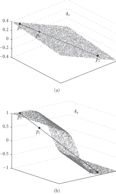
Proposition 1. Letp1andp2denote two arbitrary points lying
on a surface Sin a 3D space and let pc denote an arbitrary point lying on a straight line joiningp1andp2.Sis a plane if and only if for allp1,p2∈S,pclies onS.
An illustration ofProposition 1is shown inFigure 5. In
Figure 5(a), two pointsp1andp2are lying onSvandpcis an arbitrary point onp1p2. SinceSvis a plane (v=0.1s1+ 0.3s2
0.4 0.2 0 0.2 0.4
Sv
pc
p1
p2
(a)
1 0.5 0 0.5
1 Sx
pc
p1
p2
(b)
Figure5: An example showing the difference between a plane and a nonlinear surface. (a) A plane: arbitrary pointpc ∈ p1p2lies on Sv. (b) A nonlinear surface: the pointpc∈p1p2falls out ofSx.
sinceSx is not a plane (z = tanh(10v) = tanh(10(0.1s1+ 0.3s2)) in the example),pcdoes not lie onSx.
3.2. Transformation of a nonlinear surface to a plane
In order to construct a planeSz from a given nonlinear sur-faceSx, we propose a heuristic method that utilizes proper-ties of the straight line in a 3D space. Given anXYZ coor-dinate system, the following definitions and propositions are observed.
Definition 3. The equation of a line containing a point
p1(x1,y1,z1) can be written as (x−x1)/a = (y−y1)/b = (z−z1)/c, where a,b,c are the scalars and are not all zeros.
Definition 4. Letp1(x1,y1,z1) andp2(x2,y2,z2) be two arbi-trary points. The pair {p1,p2}is called a companion pair,
Cp1,p2, if and only ifx1 = x2 andy1 = y2. The point p1 is then called a companion ofp2and vice versa.
Proposition 2. Given an arbitrary point,p1( , ,zp1), and its companion point, q1( , ,zq1), let p2( , ,zp2)be another ar-bitrary point and let q2( , ,zq2)be its companion point. Let
pc( , ,zpc)andqc( , ,zqc)be the two arbitrary points lying on p1p2andq1q2, respectively. Ifpcis the companion ofqc, then the following expression holds true:
zpc−zp1 zp2−zp1 =
zqc−zq1
zq2−zq1. (10)
The proposition is a direct consequence of Thales’ theo-rem. Its proof is provided in the appendix.
Proposition 2 is the key of our technique. Given five pointsp1,p2,q1,q2, andpc, we can locate the position of the sixth point,qc, by using (10). Now assume that a reference
planeSv is known, and our task is to transform a
nonlin-ear surfaceSxinto a planeSz. The following transformation
scheme will detail our technique to transformSxintoSzwith
the help of the reference planeSv.
Transformation scheme
(1) Pick up any two arbitrary points p1 and p2 on the
reference planeSv. Locate their respective companion pointsq1andq2onSx.
(2) Select an arbitrary pointpconp1p2. Find a companion
point,qc∈q1q2, ofpcby using (10).
(3) LocateqxonSxsuch that{pc,qx}is a companion pair.
(4) Pullqxtowardqc.
(5) UseProposition 1to check whetherSxis a plane. (6) Repeat steps (1) to (5) if it is not a plane, otherwise
stop.
Figure 6illustrates a change of pointqxin one iteration. The old location ofqxis shown inFigure 6(a). After a
trans-formation iteration,qxis changed toqc(Figure 6(b)) which lies on the same straight line joiningq1andq2. The transfor-mation is repeated for every pointqx ∈ Sx and at the end, the surfaceSxis transformed to a planeSz.
4. gpICA ALGORITHM
In this section, the above transformation scheme will be ap-plied to create our geometric linearizing technique. However, the following issues have to be solved due to the unavailabil-ity ofs1ands2.
(1) Since the values ofs1 ands2 are not known, the first two coordinates of a point are not available. Therefore, we cannot applyDefinition 4directly to identify the companion of a given point.
(2) In PNL problem, a reference plane is also not available.
(3) The ambiguity of the point qc ∈ q1q2. Since the
first two coordinates are unknown, we cannot en-sure whether pc ∈ p1p2. Therefore, the reverse of Proposition 2does not always hold, that is, there may be more than one point that satisfy (10) but are not the companion ofpc.
1 0.5 0 0.5 1
Sx Sv
p1 pc
p2 q1
qx
q2
(a)
1 0.5 0 0.5 1
Sx Sv
p1 pc
p2 q1
qx=qc
q2
(b)
Figure6: An illustrative example of linearizingSx using reference
planeSv. (a) The pointqx∈Sxbefore transformation. (b) After the
transformation,qxwas pulled toqc∈q1q2.
t = t1, the coordinates of the corresponding points on the surfacesSv2,Sx1, andSx2 are given by (s1(t1),s2(t1),v2(t1)), (s1(t1),s2(t1),x1(t1)), and (s1(t1),s2(t1),x2(t1)), respectively. Considering PNL problem modeled by (8) and (9), the fol-lowing proposition is observed.
Proposition 3. Given the time instantt=t1, then all the points p1v( , ,v1(t1))∈Sv1,q1v( , ,v2(t1))∈Sv2,p1( , ,x1(t1))∈
Sx1, andq1( , ,x2(t1))∈Sx2are the companions.
An example ofProposition 3is shown inFigure 7. In 3D space,p1and its companionq1are shown inFigure 7(a)as the two points having the same values on the first two co-ordinates. Meanwhile, this companion property is shown in the time series plots inFigure 7(b)as the two signal samples having the same time instantt=t1. Thus withProposition 3, companion points can be identified without knowing the co-ordinatess1ands2.
For the second issue of finding a reference plane, a pro-posed solution is to employ a “fake plane,” that is, to as-sume one surface as reference plane and use it to trans-form the other surface. The role of “fake plane” will be alternatively changed from one surface to another during
1 0.5 0 0.5 1
Sx1
Sx2 p1
q1
(a)
520 510
500 490
480 1 0.5 0 0.5 1
x1
520 510
500 490
480 0.4 0.2 0 0.2
x2
t1=500 p1 q1
(b)
Figure7: Example of a companion pairCp1,q1. (a) In a 3D space,
p1andq1have the same values on the coordinatess1ands2. (b) In time series plots,p1andq1are at the same time instant.
the transformation process. For this reason, the transforma-tion process mentransforma-tioned in Section 3 is modified to adapt with the fake plane. Let us chooseSx2as the fake plane and
Sx1 as the surface that needs to be transformed. Given two pointsp1( , ,x2(t1)) andp2( , ,x2(t2)) lying onSx2and the other two points q1( , ,x1(t1)) and q2( , ,x1(t2)) lying on
Sx1, letpc be a point being located at ( , ,x2(tc)). Then the value on the third coordinate of the companion point ofpc, qc( , ,z1(tc)), can be computed from (10) as
z1tc=x2
tc−x2t1 x2t2−x2t1
x1t2−x1t1+x1t1. (11)
The last issue is the ambiguity of the pointqc ∈ q1q2.
Proposition 2implies that ifpc∈p1p2andpcandqcare the companion points, then (10) holds true, but the reverse is not always true. There may be more than one pointqcthat satisfy
1 0.5 0 0.5 1
Sx1
Sx2
p1 pc
p2 q1
qx
q2
(a)
1 0.5 0 0.5 1
Sx1
Sx2
p1 pc
p2
q1 qx
qc
q2
(b)
Figure8: An example of gpICA method. The surfaceSx1is trans-formed using the fake planeSx2. Position ofqx(a) before and (b) after the transformation. Becauseμ <1,qxis pulled to a new posi-tion nearqc.
the surface is divided into small cells and the transformation process is carried out within these cells. In addition, instead of pullingqxright toqc, we apply a learning rateμ <1 to
up-dateqxposition. By doing this way, the transformation will take a longer time but will steadily converge to a plane. The updating function is formulated as
xnew 1
tc=μz1tc+ (1−μ)x1old
tc. (12)
Figure 8shows an example of our proposed method in an iteration. The two surfacesSx1andSx2represent two non-linear mixturesx1andx2, respectively. The surfaceSx2is as-sumed to be a “fake plane” and is used to transformSx1into a plane. The position of the selected point, qx, before the change is illustrated in Figure 8(a). The new location ofqx after the change is shown inFigure 8(b). With the learning rateμ <1,qxdoes not move right toqcbut to a location near qc.
After the proposed linearizing process, we obtained two planes, Sz1 andSz2, which represent the linearized signals z1 andz2, respectively. To improve the smoothness of these surfaces, a smoothing function is applied. In this work, we use an averaging function to smooth the signals. The signal is sorted in an ascending order, and the sorted signal,zs, is
smoothed using the function
zi(t)=1L
(L−1)/2
j=−(L−1)/2 zs
i(t+j). (13)
Then ziis restored to the original order to produce signals zi. These smoothed signals,zi, are used as the inputs for the
linear ICA algorithm applied in the demixing stage.
Finally, the algorithm is extended for the case ofn > 2 observations. Each signalxi(i=1, 2,. . .,n) is represented by a surfaceSxi. In an iteration, a surfaceSxkis randomly chosen
and used as the “fake plane” to transform the other surfaces. Equation (11), therefore, is updated to
zitc=xk
tc−xkt1 xkt2−xkt1
xit2−xit1+xit1. (14)
Likewise, the updating equation (12) is modified as
xnew i
tc=μzitc+ (1−μ)xioldtc. (15)
The stopping criteria “Sx is a plane” of the transformation
scheme inSection 3also need to be realized into a precise condition in order to complete the gpICA algorithm. In this work, we measure the difference (error) between the values of the signal after and before the change in one iteration. In each iteration, these errors are accumulated and compared to a thresholdξ. The accumulated error,, is computed by
=nN1
k n
i=1 Nk
j=1
xnew
i (j)−xoldi (j)2, (16)
wherexnew
i (j) andxiold(j) are the signal values after and
be-fore the change, respectively, andNk is the number of up-dated samples in each iteration. The linearizing process is stopped when goes below a threshold ξ. After that a ba-sic linear ICA algorithm is applied on the linearized signals,
zi(i=1, 2,. . .,n), to produce the estimates of source signals, yi. A framework of gpICA is described by the following pseu-docode.
5. SIMULATION RESULTS
To evaluate the performance of gpICA, several computer simulations have been carried out on different data sets. The first test was done on a simple case of two sinusoidal sources. The sources, mixtures, and estimated signals, therefore, can be visualized in a 3D space. To assess the performance of the gpICA in a multiple-source PNL problem, we carried out the second simulation with four speech signals.
We have applied several typical linear ICA methods for the linear demixing stage (step (5)), such as SOBI (second-order blind identification) [5], JADETD (joint approximate diagonalization of eigen matrices with time delays) [23], and FPICA (fixed-point ICA) [6]. As results of these methods were almost identical, we only provide the outcomes that were carried out with SOBI during the simulation.
Input
x1,x2,. . .,xn:nobserved signals withNsamples each.
Parameter
μ: learning rate.
ξ: threshold to stop the linearization.
Nk: number of points to be updated in each iteration.
Output
z1,z2,. . .,zn:nlinearized signals.
y1,y2,. . .,yn:nestimated signals.
function gpICA()
{
Repeat{
Randomly select fake planexk.
Fori=1 ton{ Forj=1 toNk{
Randomly generate time indicest1,t2, andtc.
Computezi(tc) using (14).
Updatexi(tc) using (15).
} /∗end ofjloop∗/
} /∗end ofiloop∗/ Computeusing (16).
}Until (< ξ)
Fori=1 tonassignzi=xi.
Fori=1 tonsmoothziusing (13).
Apply a linear ICA algorithm onzito extractyi. } /∗end of gpICA∗/
Algorithm1: The Geometric PNL Algorithm: gpICA
choose SOBI, and for the PNL one, we choose Gauss-TD [15], one of the effective reported PNL methods. The perfor-mance was measured by the correlation coefficient between an original source,s, and an output signal,y. The correlation coefficient betweensandy,r(x,y), is computed by
r(s,y)=
N t=1
s(t)−sy(t)−y N
t=1
s(t)−s2N t=1
y(t)−y2, (17)
wheres = (1/N)Nt=1s(t), y = (1/N) N
t=1y(t), withNas
the number of samples.
5.1. Experiment 1: mixture of two sinusoidal signals
Using two sinusoidal signals in (18), two linear mixturesv1 andv2 were generated by a mixing matrixAwhose entries were the random numbers in the range of [−1, 1]. The linear mixtures were then distorted by two nonlinear functions in (20) to produce the observationsx1andx2. The source sig-nals, mixing matrix, and nonlinear functions are given be-low:
s1(t)=sin(0.22t),
s2(t)=sin2π(0.1t) + 6 cos2π(0.02t), (18)
A= −0.605 0.152 0.625 0.056
, (19)
x1(t)=3v1(t)3,
x2(t)=tanh10v2(t). (20)
At first, the linearizing process was run on 3000
sam-ples (N = 3000) with the window size of the smoothing
function L = 151, the learning rate μ = 0.2, and the er-ror thresholdξ =0.002. The 3D plots of the linearized sig-nals,zi, are shown inFigure 9(c)and are compared with the plots of linear mixtures,vi, (Figure 9(a)) and PNL mixtures,
xi, (Figure 9(b)). As it is expected, the graphs of gpICA’s
re-sult, zi, are similar to the graphs of unknown linear mix-tures,vi. Clearly, the nonlinearity inxihas been eliminated inzi. Whereas, some nonlinearity is still visible in the graphs (Figure 9(d)) of the competitive Gauss-TD algorithm.
In the next stage, a linear ICA method, SOBI, was applied onzito extract the estimates of original signals,yi. The plots
of these estimates, yi, are illustrated in Figure 10, together with plots of source signals, linear mixtures, PNL mixtures, and Gauss-TD and SOBI estimates. Compared with those of SOBI and Gauss-TD, gpICA’s results resemble much more to the original source signals. The linear ICA algorithm pro-vided the worst performance (Figure 10(d)). A quantitative performance was measured in terms of the correlation co-efficient between a source signal and its estimate si, r(si,si).
The estimate of theith source signal,si, is one of the out-puts yj (j = 1, 2,. . .,n) whose absolute correlation
coef-ficient, |r(yj,si)|, is the highest one. Using this index, r(si,si),
comparisons between gpICA and SOBI, and Gauss-TD were carried out and are reported in Table 1. As it is shown in the table, the result obtained by gpICA is better than both SOBI and Gauss-TD results, providing high correlation coef-ficients,|r(si,si)| ≈1.
5.2. Experiment 2: mixture of four speech signals
In this simulation, 5000 samples of four speeches (taken from [24]) were chosen as the original sources. Their linear and nonlinear mixtures are given by
A=
⎡ ⎢ ⎢ ⎢ ⎣
−0.087 0.714 −0.835 0.448 0.283 −0.560 −0.842 −0.130 −0.086 0.093 −0.061 0.522 −0.483 −0.751 0.531 0.202
⎤ ⎥ ⎥ ⎥ ⎦,
x1(t)=tanh10v1(t),
x2(t)=0.1v2(t) +v2(t)3, x3(t)=tanh2v3(t)+v3(t)3,
x4(t)=v4(t) + tanh7v4(t).
(21)
The plots of the original speeches, linear mixtures, and PNL mixtures are shown inFigure 11. Our proposed algorithm, gpICA, was executed on these PNL mixtures with parame-tersL =151,μ =0.5, andξ = 0.01. The final outputs, yi, are plotted inFigure 11(f), next to the outputs of SOBI and Gauss-TD. The correlation coefficients between the estimates
siand their original signalssiof gpICA, SOBI, and Gauss-TD
are provided inTable 2.
1 0.5 0 0.5
1 s1
1 0.5 0 0.5 1
s2 1 0.5 0 0.5 1
Sv1
Sv2
(a)
1 0.5 0 0.5
1 s1
1 0.5 0 0.5 1
s2 3 2 1 0 1 2 3 Sx
1
Sx2
(b)
1 0.5 0 0.5
1 s1
1 0.5 0 0.5 1
s2 100
50 0 50 100
Sz1
Sz2
(c)
1 0.5 0 0.5
1 s1
1 0.5 0 0.5 1
s2 3 2 1 0 1 2 3
Sz1
Sz2
(d)
Figure9: Geometric representation of signals in a 3D space. (a) Linear mixturesv1andv2. (b) PNL mixturesx1andx2. (c) gpICA’s linearized signalsz1andz2. (d) Linearized signals using Gauss-TD.
Table 1: Experiment 1: mixture of two sinusoidal signals— correlation coefficient between the original sources and their esti-mates.
Method r(s1,s1) r(s2,s2)
SOBI 0.887 0.582
Gauss-TD −0.982 0.888
gpICA −0.999 −0.966
Table2: Experiment 3: mixture of four speech signals—correlation coefficient between the original sources and their estimates.
Method r(s1,s1) r(s2,s2) r(s3,s3) r(s4,s4)
SOBI −0.404 0.816 0.590 0.695
Gauss-TD −0.770 0.984 −0.956 0.611
gpICA −0.724 0.946 −0.875 -0.926
speech signals effectively. Our proposed algorithm continued to provide good performance with high-quality estimated signals; even the poorest output of gpICA still has correla-tion coefficient of over 0.72. Compared with the Gauss-TD
algorithm which uses additional assumption of the Gaus-sianity of the mixtures, gpICA provided a similar perfor-mance.
6. CONCLUSION
A geometric approach called gpICA for the post nonlin-ear independent component analysis has been presented in this paper. By considering the characteristics of a plane and a nonlinear surface in a multidimensional space, a sim-ple linearizing process has been developed to transform the post nonlinear mixtures into linear mixtures without any additional assumption. From the linearized signals, the unknown sources can be estimated by any linear ICA algo-rithm. Throughout extensive experiments, gpICA was able to perform well in all the simulations without changing the algorithm configuration and parameters. With the two-stage separating model and a novel geometric linearizing tech-nique, gpICA possesses the following several advantages.
200 180 160 140 120 100 80 60 40 20 0 1 0.5 0 0.5 1 s1 200 180 160 140 120 100 80 60 40 20 0 1 0.5 0 0.5 1 s2 (a) 200 180 160 140 120 100 80 60 40 20 0 1 0.5 0 0.5 1 v1 200 180 160 140 120 100 80 60 40 20 0 1 0.5 0 0.5 1 v2 (b) 200 180 160 140 120 100 80 60 40 20 0 10 5 0 5 10 x1 200 180 160 140 120 100 80 60 40 20 0 1 0.5 0 0.5 1 x2 (c) 200 180 160 140 120 100 80 60 40 20 0 2 0 2 y1 200 180 160 140 120 100 80 60 40 20 0 1 0 1 y2 (d) 200 180 160 140 120 100 80 60 40 20 0 2 1 0 1 2 y1 200 180 160 140 120 100 80 60 40 20 0 3 2 1 0 1 2 y2 (e) 200 180 160 140 120 100 80 60 40 20 0 2 1 0 y1 200 180 160 140 120 100 80 60 40 20 0 1 0 1 y2 (f)
Figure10: Plots of 200 signal samples. (a) Unknown sources. (b) Linear mixtures. (c) PNL mixtures. (d) SOBI estimates. (e) Gauss-TD estimates. (f) gpICA estimates.
unlike Gauss-TD, gpICA does not use the Gaussianity assumption about the linear mixtures.
(2) The linearization and demixing processes are indepen-dent. The users can choose any suitable linear ICA algorithm for demixing stage. Thus, it increases the performance and adaptation of gpICA in a specific en-vironment.
(3) With a single fixed configuration, gpICA can perform the extraction effectively in various simulations with different data sets.
However, several issues still exist and require further investi-gations to improve the algorithm. The first issue comes from the heuristic criterion in (10). A possible solution could be another version with multiple updating points or multiple “fake planes.” The convergence conditions and the criteria for selecting the algorithm’s parameters are also other issues that need more study. Geometric approach to nonlinear ICA is not constrained to PNL model, an extended version of gpICA
for a broader nonlinear ICA submodel is being carried out. Finally, the question of whether gpICA can be applied for optimizing the data encoding (like the LOCOCODE method [10]) is an interesting issue for the future study.
APPENDIX
PROOF OFPROPOSITION 2
Since p1 and q1 are the companion points, their
coor-dinates are specified as (x1,y1,zp1) and (x1,y1,zq1), re-spectively. Similarly, p2 and q2 are located at (x2,y2,zp2) and (x2,y2,zq2), pc and qc are located at (xc,yc,zpc) and (xc,yc,zqc).
FromDefinition 3, as pclies on p1p2, we derive the fol-lowing equation:
xc−x1 x2−x1 =
yc−y1 y2−y1 =
zpc−zp1
5000 4000
3000 2000
1000 0
10 0 10
s4 5 0 5
s3 5 0 5
s2 10
0 10
s1
(a)
5000 4000
3000 2000
1000 0
5 0 5
v4 5 0 5
v3 5 0 5
v2 5 0 5
v1
(b)
5000 4000
3000 2000
1000 0
10 0 10
x4 200 20
x3 50
0 50
x2 1 0 1
x1
(c)
5000 4000
3000 2000
1000 0
0.2 0 0.2
y4 0.05
0 0.05
y3 0.2
0 0.2
y2 0.20 0.2
y1
(d)
5000 4000
3000 2000
1000 0
0.1 0 0.1
y4 0.1
0 0.1
y3 0.1
0 0.1
y2 0.05
0 0.05
y1
(e)
5000 4000
3000 2000
1000 0
0.1 0 0.1
y4 0.05
0 0.05
y3 0.05
0 0.05
y2 0.05
0 0.05
y1
(f)
Figure11: Plots of the speech signals. (a) Unknown sources. (b) Linear mixtures. (c) PNL mixtures. (d) SOBI estimates. (e) Gauss-TD estimates. (f) gpICA estimates.
Similarly, sinceqc lies onq1q2, we have the following equa-tion:
xc−x1 x2−x1 =
yc−y1 y2−y1 =
zqc−zq1
zq2−zq1. (.23)
Combining (.22) and (.23) yields
zpc−zp1 zp2−zp1 =
zqc−zq1
zq2−zq1. (.24)
REFERENCES
[1] A. Hyv¨arinen, J. Karhunen, and E. Oja,Independent Compo-nent Analysis, John Wiley & Sons, New York, NY, USA, 2001. [2] A. Cichocki and S.-I. Amari,Adaptive Blind Signal and Image
Processing, John Wiley & Sons, New York, NY, USA, 2002. [3] P. Comon, “Independent component analysis, a new
con-cept?”Signal Processing, vol. 36, no. 3, pp. 287–314, 1994.
[4] A. J. Bell and T. J. Sejnowski, “An information-maximization approach to blind separation and blind deconvolution,” Neu-ral Computation, vol. 7, no. 6, pp. 1129–1159, 1995.
[5] A. Belouchrani, K. Abed-Meraim, J.-F. Cardoso, and E. Moulines, “A blind source separation technique using second-order statistics,”IEEE Transactions on Signal Processing, vol. 45, no. 2, pp. 434–444, 1997.
[6] A. Hyv¨arinen, “Fast and robust fixed-point algorithms for in-dependent component analysis,”IEEE Transactions on Neural Networks, vol. 10, no. 3, pp. 626–634, 1999.
[7] D.-T. Pham and J.-F. Cardoso, “Blind separation of instanta-neous mixtures of non stationary sources,”IEEE Transactions on Signal Processing, vol. 49, no. 9, pp. 1837–1848, 2001. [8] P. Pajunen, A. Hyv¨arinen, and J. Karhunen, “Nonlinear blind
[9] P. Pajunen and J. Karhunen, “A maximum likelihood ap-proach to nonlinear blind source separation,” inProceedings of 7th International Conference on Artificial Neural Networks (ICANN ’97), pp. 541–546, Lausanne, Switzerland, October 1997.
[10] S. Hochreiter and J. Schmidhuber, “Feature extraction through LOCOCODE,”Neural Computation, vol. 11, no. 3, pp. 679–714, 1999.
[11] S. Hochreiter and J. Schmidhuber, “LOCOCODE performs nonlinear ica without knowing the number of sources,” in Pro-ceedings of the 1st International Workshop on Independent Com-ponent Analysis and Signal Separation (ICA ’99), pp. 149–154, Aussois, France, January 1999.
[12] C. Jutten and J. Karhunen, “Advances in nonlinear blind source separation,” in Proceedings of the 4th International Workshop on Independent Component Analysis and Signal Sep-aration (ICA ’03), pp. 245–256, Nara, Japan, April 2003. [13] A. Hyv¨arinen and P. Pajunen, “Nonlinear independent
com-ponent analysis: existence and uniqueness results,”Neural Net-works, vol. 12, no. 3, pp. 429–439, 1999.
[14] A. Taleb and C. Jutten, “Source separation in post-nonlinear mixtures,” IEEE Transactions on Signal Processing, vol. 47, no. 10, pp. 2807–2820, 1999.
[15] A. Ziehe, M. Kawanabe, S. Harmeling, and K.-R. M¨uller, “Blind separation of post-nonlinear mixtures using linearizing transformations and temporal decorrelation,”Journal of Ma-chine Learning Research, vol. 4, no. 7-8, pp. 1319–1338, 2003. [16] H. Y. Howard, S.-I. Amari, and A. Cichocki,
“Information-theoretic approach to blind separation of sources in non-linear mixture,”Signal Processing, vol. 64, no. 3, pp. 291–300, 1998. [17] A. Parashiv-Ionescu, C. Jutten, A. Ionescu, A. Chovet, and A.
Rusu, “High performance magnetic field smart sensor arrays with source separation,” inProceedings of the 1st International Conference on Modeling and Simulation of Microsystems (MSM ’98), pp. 666–671, Santa Clara, Calif, USA, April 1998. [18] S. Prakriya and D. Hatzinakos, “Blind identification of
LTI-ZMNLLTI nonlinear channel models,”IEEE Transactions on Signal Processing, vol. 43, no. 12, pp. 3007–3013, 1995. [19] M. J. Korenberg and I. W. Hunter, “The identification of
non-linear biological systems: LNL cascade models,”Biological Cy-bernetics, vol. 55, no. 2-3, pp. 125–134, 1996.
[20] T. V. Nguyen, J. C. Patra, and A. Das, “A post nonlinear geo-metric algorithm for independent component analysis,” Digi-tal Signal Processing, vol. 15, no. 3, pp. 276–294, 2005. [21] T. V. Nguyen, J. C. Patra, A. Das, and G. S. Ng, “Post
non-linear blind source separation by geometric non-linearization,” in Proceedings of the International Joint Conference on Neural Net-works (IJCNN ’05), vol. 1, pp. 244–249, Montreal, Canada, July-August 2005.
[22] J. Eriksson and V. Koivunen, “Blind identifiability of class of nonlinear instantaneous ica models,” inProceedings of the 11th European Signal Processing Conference (EUSIPCO ’02), vol. 2, pp. 7–10, Toulouse, France, September 2002.
[23] P. Georgiev and A. Chichocki, “Robust independent compo-nent analysis via time-delayed cumulant functions,” IEICE Transactions on Fundamentals of Electronics, Communications and Computer Sciences, vol. E86-A, no. 3, pp. 573–579, 2003. [24] A. Cichocki, S.-I. Amari, K. Siwek, et al., Icalab toolboxes,
2003,http://www.bsp.brain.riken.jp/ICALAB.
Thang Viet Nguyen received his B.S. de-gree in computer science from the Viet-nam National University, Hanoi, VietViet-nam, in 2000. He is currently pursuing the Ph.D. degree at the School of Computer Engineer-ing, Nanyang Technological University, Sgapore. His research interests include in-dependent component analysis, neural net-works, and genetic algorithm.
Jagdish Chandra Patraobtained the B.S. (Eng) and M.S. (Eng) degrees, both in elec-tronics and telecommunication engineering from Sambalpur University, India, in 1978 and 1989, respectively. He received his Ph.D. degree in electronics and communication engineering from the Indian Institute of Technology, Kharagpur, in 1996. Currently he is serving as an Assistant Professor in the School of Computer Engineering, NTU,
Singapore. His research interests include intelligent signal process-ing usprocess-ing neural networks, fuzzy sets, and genetic algorithms in the area of data security, sensor networks, image processing, and bioin-formatics. He is a Member of IEEE (USA) and Institution of Engi-neers (India).
Sabu Emmanuelreceived his B.E. degree (electronics and communication engineer-ing) from Regional Engineering College, Durgapur (1988), M.E. degree (electrical communication engineering) from Indian Institute of Science, Bangalore (1998), and Ph.D. degree (computer science) from Na-tional University of Singapore (2002). He is an Assistant Professor at the School of Com-puter Engineering, Nanyang Technological