Exploiting Temporal Feature Integration for Generalized Sound Recognition

Volume 2009, Article ID 807162,12pages doi:10.1155/2009/807162

Research Article

Exploiting Temporal Feature Integration for

Generalized Sound Recognition

Stavros Ntalampiras,

_{Ilyas Potamitis (EURASIP Member),}

_{and Nikos Fakotakis}

1_{Electrical and Computer Engineering Department, University of Patras, 26500 Rio-Patras, Greece} 2_{Department of Music Technology and Acoustics, Technological Educational Institute of Crete,}

Daskalaki-Perivolia, Crete 74100, Greece

Correspondence should be addressed to Stavros Ntalampiras,[email protected]

Received 13 July 2009; Revised 25 September 2009; Accepted 18 November 2009

Recommended by Douglas O’Shaughnessy

This paper presents a methodology that incorporates temporal feature integration for automated generalized sound recognition. Such a system can be of great use to scene analysis and understanding based on the acoustic modality. The performance of three feature sets based on Mel filterbank, MPEG-7 audio protocol, and wavelet decomposition is assessed. Furthermore we explore the application of temporal integration using the following three different strategies: (a) short-term statistics, (b) spectral moments, and (c) autoregressive models. The experimental setup is thoroughly explained and based on the concurrent usage of professional sound effects collections. In this way we try to form a representative picture of the characteristics of ten sound classes. During the first phase of our implementation, the process of audio classification is achieved through statistical models (HMMs) while a fusion scheme that exploits the models constructed by various feature sets provided the highest average recognition rate. The proposed system not only uses diverse groups of sound parameters but also employs the advantages of temporal feature integration.

Copyright © 2009 Stavros Ntalampiras et al. This is an open access article distributed under the Creative Commons Attribution License, which permits unrestricted use, distribution, and reproduction in any medium, provided the original work is properly cited.

1. Introduction

Humans have the ability to detect and recognize a sound event quite effortlessly. Moreover we can concentrate on a particular sound event, isolating it from background noise, for example, focus on a conversation while loud music is playing. During the last decades emphasis has been placed upon methods for automated speech/speaker recognition. This is due to the fact that speech plays an important role as regards to both human-human and human-machine interac-tions. While this area has reached the maturity of launching commercial products, the area of nonspeech audio process-ing still needs attention since it has the potential to provide solutions to a number of various applications. The domain of audio recognition is currently dominated by techniques which are mainly applied to speech technology [1]. This fact is based on the assumption that all audio streams can be processed in a common manner, even if they are emitted by different sources. In general, the goal of generalized audio recognition technology is the construction of a system that can efficiently recognize its surrounding environment

by solely exploiting the acoustic modality (computational auditory scene analysis [2]). Every sound source exhibits a consistent acoustic pattern which results in a specific way of distributing its energy on its frequency content. This unique pattern can be discovered and modeled by utilizing statistical pattern recognition algorithms. However there exists a vari-ety of obstacles that need to be tackled when such a system operates under real world conditions. When we have to deal with a large number of different sound classes, the recogni-tion performance is decreased. Moreover, the categorizarecogni-tion of sounds into distinct classes is sometimes ambiguous (an audio category may overlap with another) while composite real-world sound scenes can be very difficult to analyze. This fact has led to solutions which target specific problems while a generic system is still an open research subject.

diverse domains and properties for identifying a wide variety of sound classes. Furthermore three types of early integration methodologies are employed. We first analyze their perfor-mance before utilizing them to solve a real-world problem. The closest paper to our work is [9] which examines MPEG-7 audio standard upon the classification of ten sound cate-gories. The low-level descriptor audio spectrum projection is explained and combined with a generative approach (hidden Markov models), while the audio corpus consisted of a sound effects database. With a conventional maximum log-likelihood estimation, a class is assigned to all test samples and high recognition rates are achieved. Kim and Sikora [10] evaluate the performance of MPEG-7 Audio Spectrum Projection (ASP) descriptors which are extracted by utilizing several basis decomposition methods (principal component analysis, independent component analysis, and nonnegative matrix factorization) for automatic indexing of video sound tracks. MFCC parameters are employed in parallel while the probability density functions of both sets are estimated using continuous hidden Markov models. The data were acquired from a speech database and general sound effects library. They conclude that MFCC parameters demonstrate better performance under several practical constraints, that is, simplicity as well as time and memory consumption.

The next two approaches do not employ a generative pat-tern recognition technique but are based on either distance or heuristic measures. Wold et al. [11] present a framework for audio classification using a variety of acoustical features (loudness, pitch, brightness, bandwidth, and harmonicity). Their mean and covariance matrices are calculated over the training set while test sounds are classified using two distance measures (weighted L2 or Euclidean distance). Audio data

from various sound effects and musical instrument libraries are used to make up several sound classes which represent animals, machines, musical instruments, speech, and nature. An online audio analysis system is explained in [12] where audio recordings are identified as speech, music, silence, and several types of environmental sounds. The authors used statistical and morphological features of the temporal curves of the energy function, zero-crossing rate, and fundamental frequency while identification is based on a threshold heuristic procedure. Another kind of approach which tries to optimize the feature extraction stage with respect to a given classification problem is given in [13]. The authors apply two dissimilarity measures for selecting the time-frequency subspaces with the highest discrimination power. The outcome of their algorithm is the construction of a new wavelet packet tree. Subsequently, on the basis of this tree, the features are extracted and sent to a linear discriminant-based classifier for a three-level hierarchical classification of audio signals into ten classes. The audio database consists of 213 audio signals almost equally divided amongst artificial (113) and natural (100) sounds.

While the issue of generalized sound recognition has been addressed by quite a lot of studies, temporal integration of features has been covered by only a few studies, which are mainly focused on processing of music audio signals. In [14] Meng et al. explore the usage of two integration methods: simple statistics and autoregressive models for classification

of musical genres. Their dataset is divided into two parts: (a) 100 sound clips distributed equally among rock, classical, pop, jazz, and techno music genres and (b) 1210 music clips representative of 11 music genres. Four classifiers were used (linear mode, Gaussian with full covariance, Gaussian mixture model with full covariance, and a generalized linear model) which were trained with the first six coefficients of MFCC parameters. Joder et al. [15] utilized both early (on the feature level) and late (on the classifier level) temporal integration methodologies that are applied to the problem of musical instrument recognition on solo musical phrases. A total of 162 features of different domains are computed which are fed to the Fisher feature selection algorithm. For pattern recognition they used support vector machines and hidden Markov models while their database contained recordings of 8 different instruments which describe the main categories of instruments.

The main contribution of the present work is the appli-cation of temporal integration of features to the case of gen-eralized sound recognition. Ten audio classes were organized while feature sets of different domains were evaluated. Our database is thorough and concise after combining several well-documented professional sound effect collections which contain audio of high quality. A complete explanation is given inSection 4while we believe that there exists a need for a reference generic audio database in order to compare results between different approaches. In addition to MPEG-7 audio standard and Mel filterbank, we investigated a novel method which encompasses the usage of multiresolution analysis of audio signals using critical-band-based wavelet packets. The experimental protocol was carefully designed while the parameters of each stage were selected after con-ducting extensive experimentations. Lastly, a fusion schema which exploits three feature sets, each one temporarily inte-grated in an optimal way, is proposed. Our main objective is to study and understand the effect of temporal integration of sound parameters which belong to different domains—

frequencyandwavelet—for classifying generic sound events. Utilizing the results of this study we should be able to apply the described techniques to a number of diverse applications that generalized sound recognition technology can address.

The rest of this paper is organized as follows: inSection 2

a complete overview of the system is given along with a description of all sets of sound parameters. Section 3

describes the temporal integration methods and Section 4

explains the experimental protocol and reports detailed classification results, while our conclusions are drawn in

Section 5.

2. System Design Analysis

Testing audio corpus

Training audio corpus

Signal pre processing (dc-offset removal, windowing)

Perceptual wavelet packets

Mel filterbank

MPEG-7

Early (temporal) integration

Bases computation

from the training data

Obtain dimensions of

high variance

Maximum log-likelihood model selection

HMM construction from each class

· · ·

Multidomain audio processing

×

Figure1: Block diagram of the audio classification system.

domain are calculated. The different feature coefficients are not juxtaposed but used in parallel for constructing three separate models for each sound class. Subsequently three types of temporal integration methodologies are utilized: (a) statistical, (b) spectral, and (c) two autoregressive functions. They are applied to all three groups of descriptors while the probabilistic models are created for each group and for each temporal integration methodology. At this stage a dimensionality reduction technique was applied (principal component analysis) to the extracted feature values following MPEG-7 standard recommendation. A basis called audio spectrum basis is created out of the training data for all of the sound classes. This phase serves also the decrement of the computational complexity that is inserted during the creation of the statistical models. PCA technique has the ability to efficiently maintain the variance of the data while using a relatively small number of feature coefficients. The approach described here is equivalent to identifying asetof uncorrelated sound parameters for the specific task, instead of selecting the best individual parameters and combining them.

The probability density function of the sound categories descriptors is approximated by hidden Markov models [16]. HMMs constitute a powerful technique for modeling not only the static aspects of a feature sequence but also its temporal behavior. Finally the prediction on the test samples is made by selecting the density function which outputs the highest likelihood to have generated the particular feature sequence. The next paragraph analyzes the procedures that were followed during the different feature extraction methods.

2.1. Feature Extraction Analysis. Three types of sound

parameters were computed: (a) Mel-scale filterbank was selected because of its ability to sustain the most important information as regards human perception. (b) The MPEG-7 standard is currently considered to be the state-of-the-art methodology for automatic content-based sound

recog-nition, while (c) the third set is based on multiresolution analysis. The parameters that were used (frame, overlap, FFT size) were identical for having a reliable comparison between the sets. However a direct comparison between MFCC and MPEG-7 descriptor would not be fair since a data-dependent technique (PCA) is involved during the computation of the standard’s descriptor. Hence, we altered the algorithm as regards the MFCC extraction and replaced the discrete cosine transform (DCT) stage with PCA, inspired by Audio Spectrum Basis (ASB; seeFigure 2). PCA was also used for the extraction of our third group of parameters.

2.1.1. Audio Spectrum Projection (ASP). MPEG-7

Audio signal frames

ASE

extraction dB scaling

L2norm

÷ computationPCA basis (ASB)

×

Spectrum projection features Audio spectrum

envelope normalization

Figure2: Block Diagram of ASP extraction.

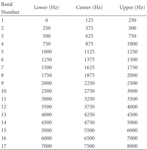
Table 1: Frequency limits used for perceptual wavelet packet integration analysis.

Band

Lower (Hz) Center (Hz) Upper (Hz) Number

1 0 125 250

2 250 375 500

3 500 625 750

4 750 875 1000

5 1000 1125 1250

6 1250 1375 1500

7 1500 1625 1750

8 1750 1875 2000

9 2000 2250 2500

10 2500 2750 3000

11 3000 3250 3500

12 3500 3750 4000

13 4000 4250 4500

14 4500 4750 5000

15 5000 5500 6000

16 6000 6500 7000

17 7000 7500 8000

2.1.2. Mel Filterbank-Based Features. For the derivation of this feature set, twenty three Mel filterbank log energies are utilized. The extraction method is the following: firstly the STFT is computed for every frame while its outcome is filtered using triangular Mel-scale filterbank. This process is proven to emphasize components which play an important role to human perception [17]. Consecutively we obtain the logarithm to adequately space the data. At this point we explore the usage of an orthogonal decomposition technique instead of DCT. PCA is employed to reduce the dimensionality of the data while projecting them on axes derived from the data. The basic kernel, which is composed of all the eigenvectors, is computed from the feature values coming from the training set. With this procedure the data are mapped onto a new coordination system based on the relationships between them. It should be noted that PCA is

adata-drivenprocedure unlike DCT which compacts data’s

energy with a standard weighting schema.

2.1.3. Perceptual Wavelet Packets Integration Analysis. Rega-rding the third feature set, we introduce the usage of critical-band-based multiresolution analysis for automated sound classification. Lately, digital signal processing using wavelets has become a common tool in many diverse research areas. Some examples are bioacoustic signal enhancement [18], applications in geophysics (tropical convection, the disper-sion of ocean waves, etc.) [19], speech/music discrimination [20], voice activity detection [21], audio coding [22], audio watermarking [23], audio fingerprinting [24], and a lot more. The main advantage of the wavelet transform is that it can process time series, which include nonstationary power at many different frequencies. The fundamental property of the Fourier transform is the usage of sinusoids with infinite duration. While they are smooth and predictable, wavelets tend to be irregular and asymmetric. They comprise a dynamic windowing technique which can treat with different precision low- and high-frequency information. The first step of the wavelet packet analysis is the choice of the original (or mother) wavelet, and by utilizing this function, the transformation breaks up the signal into shifted and scaled versions of it. In this paper we utilized Daubechies 1 (or Haar) function as the original wavelet while its optimal choice will be a subject of our future work. Unlike discrete wavelet transform (DWT), when wavelet packets (WPs) are employed, both low- and high-frequencies coefficients are kept. In our case the DWT is applied three subsequent times and consists of three-stage filtering of the audio signals as we can see inFigure 3.

The idea behind the third set is the production of a vector that provides a complete analysis of the audio signal across different spectral areas while they are approximated by WP. We should also take into account that not all parts of the spectrum affect human perception in the same way (which is crucial for sound recognition). Consequently, the division of the spectrum requires a fine partitioning. In [25, 26] it is observed that the human auditory system filters the entire audible spectrum into many critical bands. Based on this observation, we employed a critical-band-based filterbank with the frequency ranges denoted in

Input audio

signal Gabor filters, critical band

analysis CB1 CB2 . . . CB17

For each spectral band

· · ·

D1

A1 Wavelet packet

transform, Daubechies 1

(Haar)

DD2

AD2

DA2

AA2

DDD3 ADD3 DAD3 AAD3 DDA3 ADA3 DAA3 AAA3

For each wavelet

packet coefficient

· · ·

Segmentation and autocorrelation

calculation

Area under envelope of autocorrelation

Output feature vector

Figure3: Perceptual wavelet packet integration audio analysis.

then segmented and the autocorrelation envelope area is computed and normalized by half the segment size. N -normalized integration parameters are calculated for each frame, whereNis the total number of the frequency bands multiplied by the number of the wavelet coefficients (17×

8 = 136). This series of parameters comprises the PWP-integration feature vector and the entire calculation process is depicted in Figure 3. These parameters reflect upon the degree of variability of a specific wavelet coefficient within a frequency band. Since the audio signals we try to classify exhibit great differences among the critical bands, we decided to utilize the normalized autocorrelation envelope area.

2.2. Construction of Probabilistic Models. Automatic sound recognition is based on the assumption that each sound event follows a distinct pattern across different frequencies, which is often called audio signature. The aforementioned audio feature vectors try to capture this property and, subsequently, can be utilized by statistical pattern recognition algorithms in order to be used to categorize unknown sound events. A powerful technique that approximates the probability density function which is followed by the descriptor values is hidden Markov models. With this procedure a probabilistic model is constructed for each sound class using the training data. This model contains the a priori knowledge that we have about the class, and as long as the data are representative of the particular sound class, the model is considered to be an adequate description of such audio events. Unlike Gaussian mixture models which do not have the ability to model the temporal evolution of a sound, HMMs break up the feature sequence into a predefined number of states and learn the associations between them. This results in a

k ×k transition matrix whereas each one of its elements reflects upon the probability of transition across different states. Thus, the element (i, j) is the probability of moving to state jat timet+ 1 given stateiat timet. In the current paper we use left-right HMMs which means that there are no directed loops in the automation while the distribution of each state is modeled by one GMM with diagonal covariance matrix. During classification the trained models are used

for computing a degree of resemblance (e.g., log likelihood) between each model and an unknown input signal. The model that generates the highest probability comprises the system’s prediction regarding the input signal. This pattern recognition technique belongs to the generative approaches, whose main property is that they handle the samples of each class independently of the other classes.

Torch [27] implementation of HMM, written in C++, was used during training and testing. The maximum number of k-means iterations for initialization was 50 while the Baum-Welch algorithm had and upper limit of 25 iterations with a threshold of 0.001 between subsequent iterations. Extensive experiments were conducted: (a) for constructing the model of each sound class with respect to each feature set, (b) to test each temporal integration method, as well as to (c) decide on the size of the temporal integration window (the number of frames that were merged). In particular the range of the number of states was between 3 and 7 while the numbers of Gaussian components tested, respectively, was

{2, 4, 8, 16, 32, 64, 128}. The final values of these parameters were chosen using the highest recognition rate criterion.

3. Strategies for Temporal Feature Integration

frames to be integrated with respect to audio feature sets of different domains as well as various integration strategies.

More specifically, we study the effect of temporal integra-tion of features in order to achieve a global representaintegra-tion of an audio sequence using a smaller number of time instances. By integrating the features in the temporal sense we capture a more characteristic-global view of the signal which can be more representative than frame values of small duration. Thus the within-class variability is reduced which results in finer modeling of the shared characteristics amongst the samples of the same sound category. The time slot over which the integration takes place is called texture window. This technique belongs to theearlyintegration category since the integration does not take place on the classifier level but on the feature extraction level.

Each integration function is applicable to a predefined number of frames and transforms them according to the following equation:

Xk=F

xt,. . .,xt+p−1

, (1)

where Xk denotes the integrated vector of thekth texture

window and xi is the value of feature x at frame t. The

number of frames over which the integration is applied is denoted as p. This equation provides a higher-level description of the feature series. Several integration strategies are based on the computation of statistics over the texture window. Other strategies are based on the assumption that the feature sequence can be viewed as a random process (e.g., autoregressive models). The three different integration strategies which are investigated in this work are explained below.

3.1. Computation of Short-Term Statistics. A relatively simple way to merge the information which is provided by many subsequent frames into one is the computation of their statistical instances. We consider the next five statistical measurements: mean (or expected value), variance, median, as well as the first and third quartiles over each texture window. Although they are relatively simple to calculate, they can be representative of the feature sequence. Except for mean and variance, which are of high importance (see [30,

31]), we also make use of three percentiles. They reflect upon the value below of which a certain percent of observations may be found. The first, second (median), and third quartiles correspond to 25, 50, and 75 percent, respectively. The short-term statistics integration function is the following:

Fstat

xt,. . .,xt+p−1

=meanxt,. . .,xt+p−1

, varxt,. . .,xt+p−1

,

q1xt,. . .,xt+p−1

,. . ., medianxt,. . .,xt+p−1

,

q3xt,. . .,xt+p−1

.

(2)

Its outcome is a vector with size five times the initial dimension (R = 5×D). The main disadvantage of simple statistics is their inadequacy to capture the dynamicity

of an audio signal since another combination of several observations can result in the same integrated vector. The next two integration strategies share the fact that they try to capture the temporal behavior of a given series.

3.2. Spectral Moments. The temporal dependency between

successive feature observations can be extracted using the information provided by the spectrum of these features. The method employed here was used in [14] for automatic musical genre classification and is an extension of the modulation energy of several features used by McKinney and Breebaart [32]. Initially the STFT of the sound parameters is calculated over the texture window. Its outcome forms the basis for calculating the spectral moments and includes the entire information which is provided by the spectrum of each feature. In this way we can determine the sinusoidal frequency and phase content of local sections of a given feature sequence as it changes over time. It should be noted that here another parameter is inserted; the size of the FFT which is irrelevant to the FFT employed by the feature extraction algorithms comprises the number of frames that can be included in the texture windows.

First, the power spectrum in dB of the series of a particular descriptor is calculated and its mean value μ is stored. Subsequently the next four statistics over the texture size of the amplitude spectrum are calculated: the mean

m, variance v, skewness γ, and kurtosis κ. The last two measurements are taken because they basically express the dispersion of the instance across their expected value. If skewness is negative, the data are spread out more to the left of the mean than to the right. If skewness is positive, the data are spread out more to the right. For a perfectly symmetric distribution, it is zero. Kurtosis describes the pdf of a random variable while emphasis is placed upon the deviation that its variance exhibits. If the case is that the variance exhibits infrequent extreme deviations, then kurtosis is more than 3. On the contrary when the variance is of frequent small-sized deviations, kurtosis is characterized by lower values. Conclusively the final integrated vector has five times larger dimension than the starting one like the previous strategy (R=5×D) as

Fspec

xt,. . .,xt+p−1

=μ,m,v,γ,κ. (3)

3.3. Autoregressive Models (AR). Another methodology for

the coefficients of an autoregressive model of order O is shown below:

x[t]=w+

O

n=1

x[t−n]An+et, (4)

wherewis the intercept vector,Anare theD×Dcoefficient

matrices of the autoregressive model, andetis a white noise

vector of dimensionD. Thus the integrated feature vector is

FMAR

xt,. . .,xt+p−1

= w,A1,. . .,

AO

, (5)

which is of dimensionR =D(O×D+ 1). The same least-square approximations are computed for the case of DAR but a further assumption is made: the sound descriptors are independent with respect to each other. As a result the constraint exists that the model coefficients should be diagonal matrices. Hence, we calculate the parameters for each feature alone each time and the outcomes are concatenated. In this case we have a vector of significantly lower dimension,R=D(O+ 1), as

FDAR

xt,. . .,xt+p−1

= w,D1,. . .,

DO

. (6)

4. Experimental Setup and Comparative

Evaluation

This section covers the details regarding both testing and training phases of our experimentations. Our aim is to assess the performance of the three different feature sets on the same database when they have been temporarily integrated. For each classification stage the left-right HMMs were optimized in terms of number of states and components. The data were split into 70% for training and 30% for testing in a random way while these sequences were the same for all stages. Our corpus consists of audio acquired from professional sound effects collections which are of high quality and are mainly employed by the movie industry. They are used to process or even replace the audio stream that was recorded at the actual scene. These sources combined com-prise a vast corpus of vocal and nonvocal audio events which can be utilized for the construction of trained probabilistic classification models. We should underline the fact that there is a need for a common database in order to be able to directly compare the performance of different frameworks. We believe that the audio corpus used here has the potential to become a reference database which is essential for reliable comparison of related papers. Our corpus is acquired from the following collections: (i) BBC Sound Effects Library, (ii) Sound Ideas Series 6000, (iii) TIMIT, and (iv) Sony Sound Effects Library. The following ten audio classes were organized: bird call, applause, dog bark, explosion, footstep, cat meowing, gunshot, speech of both genders, laughter, and telephone ring. Our intention was to have as many common categories to previous studies as possible. A dataset that would be fully identical with other publications could not be formulated due to the different databases that have been utilized in other papers and/or their unavailability. The main

Table2: Statistics of the final dataset.

Audio category No. of sound Duration (sec) samples

Bird call 55 7,913.4

Applause 64 1,467.5

Dog barking 102 1,103.6

Explosion 131 1,803.9

Foot step 152 4,865.5

Cat meowing 141 977.1

Gunshot 187 2,290.8

Male and female

1680 5,174.4

Speech

Laughter 118 941.64

Telephone 89 1,629.59

Total 2719 28,167.4

difference is that we decided not to use the category glass smash (as used in [9]) since glass breaking sounds are present in many explosion sound events. Instead, we decided to add another animal sound category: cat meowing. Care has been taken in order to include sounds from all the databases in both train and test sets so that the models do not depend on the acoustics conditions of each database. Statistics of the final corpus are tabulated in Table 2. The sound files were downsampled to 16 KHz with 16-bit quantization while they were preprocessed so that any possible dc offset would be canceled. The databases were exhaustively searched for samples that correspond to our problem and all the relevant parts were identified and isolated for later usage. Our main concern was for the sample to be “clean” without any type of background noise. Lastly a statistical-model-based silence elimination algorithm described in [34] was used so that the pdf estimation techniques can elaborate on the structure of a particular sound event alone.

4.1. Parameters for Feature Extraction and Temporal

Inte-gration. Following the MPEG-7 standard recommendation,

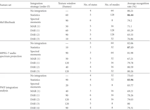
Table3: System’s performance with respect to each feature set and the integration window with the best accuracy.

Feature set Integration

strategy (orderO)

Texture window

(frames) No. of states No. of modes

Average recognition rate (%)

Mel filterbank

No integration — 4 64 80.21

Statistics 60 5 128 86.44

Spectral

moments 90 6 8 79.2

MAR (1) 50 5 16 71.1

DAR (1) 60 5 128 85.29

DAR (2) 90 5 128 83.55

DAR (3) 10 6 32 76.86

MPEG-7 audio spectrum projection

No integration — 5 64 82.06

Statistics 10 3 32 87.13

Spectral

moments 90 3 64 81.98

MAR (1) 50 5 32 67.21

DAR (1) 120 3 16 79.78

DAR (2) 40 4 16 80.59

DAR (3) 120 5 32 80.26

PWP integration analysis

No integration — 4 32 75.63

Statistics 90 4 32 83.96

Spectral

moments 20 5 8 83.77

MAR (1) 40 3 16 69.21

DAR (1) 90 6 16 78.26

DAR (2) 120 4 16 79.03

DAR (3) 120 5 8 80

DAR (4) 90 4 8 79.31

length for integrating a given feature sequence using the spectral moments strategy was set to 128. In this way the system can integrate up to 128 frames which corresponds to about 2.5 seconds. The values of the frames that are to be integrated into a texture window were taken from the set

{10, 20, 30, 40, 50, 60, 90, 120} while a constant hop size of 10 frames was adopted, so that the final number of texture windows was kept the same independently of the included number of frames. In case the sound sample is of smaller duration, then it is integrated into one texture window only. It should be mentioned that for each experimental phase the performance of the system is measured using per frame (or texture window) analysis. For the MAR method the lower limit of frames that are to be integrated is 30 since this method requires a larger number of subsequent observations for estimating the model coefficients.

4.2. Classification Results. This section presents the classifica-tion results over the different levels of our study. We first compare the performance of the feature sets that were emp-loyed to model each sound class as well as the integration strategy. Subsequently the effect of the length of the texture window is discussed. Finally we draw our conclusions as

re-gards the integration strategy that provides the best per-formance in terms of both computational complexity and recognition rate. The performance of the system with respect to each feature set using the texture window length that provided the best average recognition rate is tabulated in

confirm that MPEG-7 audio protocol provides for each audio class a representation that follows a consistent pattern which can be modeled by left-right HMMs and used afterwards for classification of novel data.

A property that is shared by all the groups of the sound parameters is that they exhibit their best performance when the short-term statistics method for temporal integration is employed. Although this method is relatively simple and does not take under consideration the possibility of temporal dependency among the feature values, it was proven to enhance the recognition performance in a domain indepen-dent way. The spectral moments method demonstrates the second best results as regards PWP integration and MPEG-7 ASP descriptors on the contrary to Mel-filterbank-based set where this is achieved by the first-order DAR method. The lowest recognition rates across all feature sets are given by the MAR method: 71.1%, 67.21%, and 69.29% for Mel, MPEG-7, and PWP groups, respectively, despite its high dimensionality needs.

Furthermore it should be emphasized that the classifiers which are trained on temporarily integrated data perform better in almost every case (exception is the MAR method). This clearly reveals that the integrated vector better captures the aspects of an audio class which are needed for recog-nition. The improvement reaches 6.23%, 5.7%, and 8.33% for Mel, MPEG-7, and PWP integration sets, respectively. Thus the usage of temporal integration techniques is useful for generalized sound recognition unlike musical instrument classification where almost identical results are obtained [15].

An interesting observation is that as we increase the order of the autoregressive processes we obtain lower classification accuracies as regards Mel and MPEG-7 sets. However the PWP integration set was providing better performance, so we decided to carry out an additional experiment using a 4th-order DAR model. Unfortunately this process provided lower accuracy than the 3rd-order one. These facts lead to the conclusion that autoregressive functions are not able to capture the temporal behavior of the feature sequence of an audio signal.

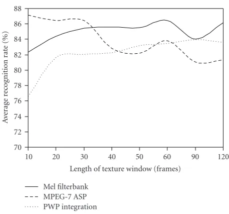
One can make the logical assumption that the larger the value of the integration window, the higher the recognition rates will be, since more information can be exploited. However this assumption is not true in every case. During this phase of the experimental results analysis, we isolated the best recognition rate for each texture window with respect to each group of parameters according to the short-term statistics method. Figure 4illustrates the variation that the average recognition rate exhibits when the length of the texture window changes. The set based on multiresolution analysis exhibits a big improvement as the length increases up to the value of 90 frames and then the performance falls. The opposite case is that of the MPEG-7 ASP descriptor where its maximum discrimination capability is when only 10 frames are integrated. Mel filterbank comprises the intermediate case while it presents maximum performance when 60 frames are integrated. During our experimentations the number of the training texture windows that were employed for HMM construction was constant due to the fixed value

70 72 74 76 78 80 82 84 86 88

A

ver

age

rec

og

nition

rat

e

(%)

10 20 30 40 50 60 90 120

Length of texture window (frames) Mel filterbank

MPEG-7 ASP PWP integration

Figure4: Average recognition rate as a function of the length of texture window with respect to each feature set.

of the hop size; hence, we avoided overfitting because of insufficient data.

Figure 5depicts the classification results in more details as regards the best overall performance that each feature set achieved. As we can see there are some sound classes that are recognized with high accuracy by all the groups of descriptors, like explosion, speech, and laughter sound events. On the other hand several sound events are correctly classified by one or two feature sets but not by the third one. Mel filterbank demonstrated its best performance in speech (98%) and bird call (94.44%) classification while it cannot recognize cat meowing (75.77%) and footstep (78.34%) sound events adequately. ASP descriptor recognized correctly all (100%) sound samples of speech and dog bark categories but achieved the lowest rate as regards the bird call class. We obtained the highest score for footstep sound recognition from the group of descriptors which is based on wavelet packet analysis. These observations indicate that the feature sets share some common characteristics but exhibit many differences when it comes to discriminate particular sound classes. Hence we decided to explore the usage of several fusion techniques which elaborate on the HMMs outputs. This experimental phase is described in the next paragraph.

0 20 40 60 80 100 Bi rd ca ll Ap p la u se Dog bar k Explosion Fo o ts te p Cat m eo w G u nshot _Speec h Laug ht er Te le p h o n e

94.44 92.3 _{88 91}.11

78.34 75.77 79.07 98

84.9 82.5

(a) Mel-filterbank-based feature set

0 20 40 60 80 100 Bi rd ca ll Ap p la u se Dog bar k Explosion Fo o ts te p Cat m eo w G u nshot _Speec h Laug ht er Te le p h o n e

73.27 82.61 100

81.22 87.32 82.85 82.54 100 94.34 87.14

(b) MPEG-7 audio spectrum projection

0 20 40 60 80 100 Bi rd ca ll Ap p la u se Dog bar k Explosion Fo o ts te p Cat m eo w G u nshot _Speec h Laug ht er Te le p h o n e

89 86.92 75.2

87.95 88.73

74.07 76.55 99.41

83.49 _78.23

(c) Perceptual wavelet packet integration analysis

Figure5: Recognition rates per sound class for (a) Mel filterbank, (b) MPEG-7 ASP, and (c) PWP Integration sets using the param-eters (length of texture window, number of states, and number of modes) that demonstrated the best overall accuracy.

4.3. Fusion of HMM Outputs. Following the conclusions of

the previous section we experimented on fusing the outputs of the HMMs build by utilizing different feature sets which are integrated over the texture window length that provided the highest recognition rate. The same data were used during both training and testing procedures. The difference is that instead of having sequences of features, this time we only elaborated on the probability that is generated by each HMM. We evaluated the performance of two fusion schemes: J48 tree and multilayer perceptron [35]. Decision trees can be easily constructed in a supervised way while no assumption is made a priori about the distribution of the data. Their main disadvantage is that slight alterations of the training set can result to a decision tree structure that exhibits a large number of differences. However we reduce this risk since we elaborate on probabilities of feature sequences and not on the features themselves. Multilayer perceptron (MLP) method follows the logic of the linear perceptron while it employs nodes with nonlinear activation functions for discriminating data that are not linearly separable. Additionally, artificial neural networks can be very useful where the patterns are

Table 4: Average recognition rates reached by the four fusion methods.

Fusion method Recognition rate (%)

Majority voting 79.48

Simple concatenation 85.12

(no temporal integration) (4 states, 32 modes)

J48 tree 95.67

MLP 96.95

not evident. The backpropagation algorithm was used to train the neural network with one hidden layer of twenty nodes (half the total of the number of features plus the number of classes) at a learning rate of 0.3. These methods were chosen because of their ability to handle redundant data, which means that in the case where the feature sets capture overlapping information of the acoustic signal that they represent, the algorithm can effectively exploit it and the performance of the recognizer is usually increased when compared to employing each feature set alone. A redun-dant feature set may provide improved performance under adverse conditions (where parts of the signal’s spectrum are absent or distorted) as in the case of real life. Two simpler approaches were also evaluated: majority voting and simple concatenation of all the parameters before the temporal integration stage. Regarding the case of majority voting, if an agreement was not reached, that is, if we resulted into having three different decisions for the same test sequence, then the decision was made in a random way.

In Table 4 the average recognition rates that were achieved while fusing the HMM outputs with four different methods are illustrated. The highest performance is reached by MLP-based fusion (96.95%) while the J48 decision tree method reached the second best score (95.67%). The HMMs that were constructed by concatenating all the feature sets into one provided a considerable improvement of 3.06% when compared to the MPEG-7 set alone (82.06%). The majority voting method exhibited the worst performance (79.48%) since it suffers from the fact that the first-stage HMM classifiers tend to disagree.

A direct comparison of the proposed framework with other sound classification systems is not feasible due to the different datasets that are employed by each of these works. In [9] they use the MPEG-7 ASP feature set without temporal integration reaching 82.06% on our dataset, which is considerably lower than the recognition rate achieved by the MLP-based fusion scheme.

Table5: Confusion matrix of the final system with MLP-based fusion of probabilities (%).

Presented

Responded Bird

Applause Dog barking Explosion Footstep Cat Gunshot Speech Laughter Telephone

call meowing

Bird call 95.3 0 0 0 0 2.7 2 0 0 0

Applause 0 100 0 0 0 0 0 0 0 0

Dog

0 0 96.2 0 0 0 0 0 4.8 0

barking

Explosion 0 0 0 94.89 0 2.11 3 0 0 0

Footstep 0 0 0 0 97.52 0 2.28 0 0 0

Cat

0 1.1 1.5 0 0 95.4 0 1.3 0 0.7

meowing

Gunshot 0 0 0 2.1 0 0.1 97.8 0 0 0

Speech 0 0 0 0 0 0 0 100 0 0

Laughter 0 1.2 0 0 0 0.6 1.3 0 96.9 0

Telephone 0 0 0 0 0 3.2 1.3 0 0 95.5

5. Conclusions

A framework for generalized sound recognition which leads to high accuracy was proposed. A combination of several well-documented sources of high quality was employed for coming up with a thorough dataset. The merits of temporal feature integration were exhibited as regards different audio features. The experimental protocol was carefully designed and all the aspects of the suggested methodology were evaluated in details. The results reveal that different texture windows are appropriate for each feature set while the temporal integration strategy based on short-term statistics demonstrated the best average recognition rates. The rest of the techniques, although more complex and computational intensive, could not provide a representation of the structure of the audio signals that can be modeled and subsequently identified efficiently. The first stage of the system utilizes left-right HMMs for estimating the distribution of the features that belong to each sound class. Following the outcomes of the extensive experimentations, a further step was investigated: the concurrent usage of sound parameters based on spectral and multiresolution analysis. The MLP-based fusion scheme elaborated on the probabilities that were generated by the previously constructed HMMs and provided high classification rates as regards to all the sound categories that were considered in our study. This indicates that automated generalized sound recognition is better addressed while utilizing multidomain groups of descriptors. Sound classes which are currently not included in our work can be easily incorporated as long as a sufficient amount of training data is collected. The same methodology can be used for processing the unseen audio sequences (feature extraction with temporal integration) and a probabilistic model for each new sound class can be constructed. The proposed implementation is flexible and can facilitate many sound recognition applications.

The aim of this work was the evaluation of various integration techniques for automatic audio classification.

The objective now is to use the results reported in this work to build up autonomous systems able to form an accurate description of the surrounding space based solely on their “auditory sense”. Such systems could ease our everyday life by providing solutions to a number of real-world applications. Our next step is to integrate the proposed methodology into the framework of the Prometheus project which aims at the analysis of human behavior in unrestricted environments, including recognition of their activities using heterogeneous sensors.

Acknowledgment

This work was supported by the EC FP 7th Grant Prometheus 214901 “Prediction and Interpretation of human behaviour based on probabilistic models and heterogeneous sensors”.

References

[1] J. Foote, “Overview of audio information retrieval,” Multime-dia Systems, vol. 7, no. 1, pp. 2–10, 1999.

[2] D. Wang and G. J. Brown,Computational Auditory Scene Anal-ysis: Principles, Algorithms and Applications, Wiley-Blackwell, Oxford, UK, 2006.

[3] A. T. Watson, M. A. O’Neill, and I. J. Kitching, “A quali-tative study investigating automated identification of living macrolepidoptera using the Digital Automated Identification SYstem (DAISY),”Systematics and Biodiversity, vol. 1, no. 3, pp. 287–300, 2003.

[4] K. J. Gaston and M. A. O’Neill, “Automated species identifica-tion: why not?”Philosophical Transactions of the Royal Society B, vol. 359, no. 1444, pp. 655–667, 2004.

[5] C.-H. Lee, C.-H. Chou, C.-C. Han, and R.-Z. Huang, “Automatic recognition of animal vocalizations using averaged MFCC and linear discriminant analysis,”Pattern Recognition Letters, vol. 27, no. 2, pp. 93–101, 2006.

[7] G. Tzanetakis and P. Cook, “Musical genre classification of audio signals,” IEEE Transactions on Speech and Audio Processing, vol. 10, no. 5, pp. 293–302, 2002.

[8] S. Chu, S. Narayanan, and C.-C. Jay Kuo, “Content analysis for acoustic environment classification in mobile robots,” in Proceedings of the AAAI Fall Symposium, Aurally Informed Performance: Integrating Machine Listening and Auditory Pre-sentation in Robotic Systems, Arlington, Va, USA, 2006. [9] M. Casey, “MPEG-7 sound-recognition tools,”IEEE

Transac-tions on Circuits and Systems for Video Technology, vol. 11, no. 6, pp. 737–747, 2001.

[10] H. G. Kim and T. Sikora, “Comparison of MPEG-7 audio spectrum projection features and MFCC applied to speaker recognition, sound classification and audio segmentation,” inProceedings of IEEE International Conference on Acoustics, Speech, and Signal Processing (ICASSP ’04), Montreal, Canada, May 2004.

[11] E. Wold, T. Blum, D. Keislar, and J. Wheaton, “Content-based classification, search, and retrieval of audio,”IEEE Multimedia, vol. 3, no. 3, pp. 27–36, 1996.

[12] T. Zhang and C.-C. J. Kuo, “Content-based classification and retrieval of audio,” inProceedings of the 43rd Annual Confer-ence on Advanced Signal Processing Algorithms, Architectures, and Implementations VIII, Proceedings of SPIE, San Diego, Calif, USA, July 1998.

[13] K. Umapathy, S. Krishnan, and R. K. Rao, “Audio signal feature extraction and classification using local discriminant bases,” IEEE Transactions on Audio, Speech and Language Processing, vol. 15, no. 4, pp. 1236–1246, 2007.

[14] A. Meng, P. Ahrendt, J. Larsen, and L. K. Hansen, “Temporal feature integration for music genre classification,”IEEE Trans-actions on Audio, Speech and Language Processing, vol. 15, no. 5, pp. 1654–1664, 2007.

[15] C. Joder, S. Essid, and G. Richard, “Temporal integration for audio classification with application to musical instrument classification,”IEEE Transactions on Audio, Speech and Lan-guage Processing, vol. 17, no. 1, pp. 174–186, 2009.

[16] L. R. Rabiner, “Tutorial on hidden Markov models and selected applications in speech recognition,”Proceedings of the IEEE, vol. 77, no. 2, pp. 257–286, 1989.

[17] B. Verma and M. Blumenstein,Pattern Recognition Technolo-gies and Applications: Recent Advances, Information Science Reference, 2008.

[18] Y. Ren, M. T. Johnson, and J. Tao, “Perceptually motivated wavelet packet transform for bioacoustic signal enhancement,” Journal of the Acoustical Society of America, vol. 124, no. 1, pp. 316–327, 2008.

[19] C. Torrence and G. P. Compo, “A practical guide to wavelet analysis,”Bulletin of the American Meteorological Society, vol. 79, no. 1, pp. 61–78, 1998.

[20] E. Didiot, I. Illina, O. Mella, D. Fohr, and J.-P. Haton, “A wavelet-based parameterization for speech/music segmenta-tion,” in Proceedings of the European Conference on Speech Communication and Technology (Interspeech ’06), Pittsburg, Pa, USA, September 2006.

[21] J. F. Wang and S. H. Chen, “A voice activity detection algorithm based on perceptual wavelet packet transform and Teager energy operator,” in Proceedings of the International Symposium on Chinese Spoken Language Processing (ICSLP ’02), Taipei, Taiwan, August 2002.

[22] M. Erne, G. Moschytz, and C. Faller, “Best wavelet-packet bases for audio coding using perceptual and rate-distortion criteria,” in Proceedings of IEEE International Conference on

Acoustics, Speech, and Signal Processing (ICASSP ’99), Phoenix, Ariz, USA, March 1999.

[23] X. Quan and H. Zhang, “Perceptual criterion fragile audio watermarking using adaptive wavelet packets,” inProceedings of the International Conference on Pattern Recognition (ICPR ’04), Cambridge, UK, August 2004.

[24] S. Baluja and M. Covell, “Waveprint: efficient wavelet-based audio fingerprinting,”Pattern Recognition, vol. 41, no. 11, pp. 3467–3480, 2008.

[25] B. Scharf, “Critical bands,” inFoundations of Modern Auditory Theory, J. V. Tobias, Ed., vol. 1, pp. 157–202, Academic Press, New York, NY, USA, 1970.

[26] W. A. Yost, Fundamentals of Hearing, Academic Press, New York, NY, USA, 3rd edition, 1994.

[27] Torch Machine Learning Library,http://www.torch.ch. [28] J.-J. Aucouturier, B. Defreville, and F. Pachet, “The

bag-of-frames approach to audio pattern recognition: a sufficient model for urban soundscapes but not for polyphonic music,” Journal of the Acoustical Society of America, vol. 122, no. 2, pp. 881–891, 2007.

[29] K. E. Maleh, A. Samouelian, and P. Kabal, “Frame level noise classification in mobile environments,” inProceedings of IEEE International Conference on Acoustics, Speech, and Signal Processing (ICASSP ’09), Phoenix, Ariz, USA, March 2009. [30] G. Tzanetakis, G. Essl, and P. Cook, “Audio analysis using

the discrete wavelet transform,” inProceedings of the WSES International Conference on Acoustics and Music: Theory Applications, Skiathos, Greece, September 2001.

[31] M. K. S. Khan, W. G. Al-Khatib, and M. Moinuddin, “Automatic classification of speech and music using neural networks,” inProceedings of the 2nd International Workshop on Multimedia Databases, Washington, DC, USA, November 2004.

[32] M. F. McKinney and J. Breebart, “Features for audio and music classification,” inProceedings of the International Symposium on Music Information Retrieval, pp. 151–158, 2003.

[33] T. Schneider and A. Neumaier, “Algorithm 808: ARFIT— a Matlab package for the estimation of parameters and eigenmodes of multivariate autoregressive models,” ACM Transactions on Mathematical Software, vol. 27, no. 1, pp. 58– 65, 2001.

[34] J. Sohn, N. S. Kim, and W. Sung, “A statistical model-based voice activity detection,”IEEE Signal Processing Letters, vol. 6, no. 1, pp. 1–3, 1999.