ABSTRACT
RANSHOUS, STEPHEN MICHAEL. Scalable Algorithms for Mining Dynamic Graphs and Hypergraphs with Applications to Anomaly Detection. (Under the direction of Dr. Nagiza F. Samatova.)
Graph data mining has become a ubiquitous tool for researchers and practitioners in numerous domains, including social sciences, financial markets, and computer security. In particular, mining dynamic graphs has gained substantial interest in the past decade, due to their robust expressiveness and natural ability to represent complex relationships that evolve over time. Traditional graph mining tasks, such as community detection, frequent subgraph mining, and anomaly detection, often operate on entire graph snapshots at a time, where a snapshot may consist of an entire day or week of activity. However, as the volume and velocity of data continues to increase, it is no longer feasible to analyze entire datasets at once, or even assume that the datasets will fit into memory. In this work we focus on developing efficient algorithms for mining dynamic graphs. We use anomaly detection as an exemplar task, but believe that our cross-cutting ideas and applications of efficient data structures apply much more broadly.
We propose two changes for how anomaly detection is performed over large-scale dynamic graphs to cope with the growing constraints. First, we transition from the traditional approach of analyzing graph streams, where each object in the stream is a full graph, to analyzing graph edgestreams. An immediate benefit of this transition is a smaller unit of analysis, as well as more fine-grained attribution for anomalies. Second, instead of storing exact information, we utilize approximation, heuristics, and probabilistic data structures for retaining the salient information from the stream. This results in dramatically reduced time and space complexities for our algorithms. In this dissertation we develop anomaly detection algorithms for increasingly complex graph edge stream models and show their effectiveness, both theoretically and empirically.
In our first component, based on our extensive survey and gap analysis of the field, we begin with the simplest case, undirected graph edge streams. Key graph properties necessary for our anomaly detection algorithm are approximated from the stream using Count-Min (CM) sketches. Theoretical and empirical results show that the error of our approximations is minimal, while enabling constant time operations. Experiments on synthetic and real-world datasets show the effectiveness of our approach, yielding high precision and recall, as well as interesting case studies.
no longer use CM sketches. Instead, we use MinHash and locality sensitive hashing to quickly and accurately estimate historical vertex co-occurrences. Experimental results show processing speedups between 33-750x compared to exact analysis, while maintaining comparable accuracy.
©Copyright 2018 by Stephen Michael Ranshous
Scalable Algorithms for Mining Dynamic Graphs and Hypergraphs with Applications to Anomaly Detection
by
Stephen Michael Ranshous
A dissertation submitted to the Graduate Faculty of North Carolina State University
in partial fulfillment of the requirements for the Degree of
Doctor of Philosophy
Computer Science
Raleigh, North Carolina 2018
APPROVED BY:
Dr. Dennis R. Bahler Dr. R. Raju Vatsavai
Dr. Steffen Heber Dr. Nagiza F. Samatova
DEDICATION
BIOGRAPHY
ACKNOWLEDGEMENTS
Completing this dissertation would not have been possible without the guidance, support, and encouragement from a number of people and institutions. Above all, I am eternally grateful to my advisor, Dr. Nagiza Samatova, without whom I would not have become the person and researcher I am today. Her enthusiasm and drive in has been infectious, and helped raise me to levels I did not think possible. By always placing her students first, she created a cooperative and collaborative environment that fostered intellectual growth, teamwork, and personal development.
In addition, I am grateful to all the faculty at NCSU that helped me along the way. In particular I would like to the members of my PhD committee, Professors Steffen Heber, Raju Vatsavai, and Dennis Bahler, for their valuable time and insightful feedback regarding my dissertation. I would also like to thank Dr. Douglas Reeves for my admission into the program and initial financial support.
Throughout my completion of this dissertation, I have been fortunate to have a number of collaborations with exceptionally gifted researchers, spread across top institutions across the nation. I would like to thank Tom Peterka at Argonne National Laboratory, for helping ease my transition from academics into my first true multi-disciplinary environment. I would like to thank Danai Koutra and Dr. Christos Faloutsos from CMU for their contributions to the survey performed in Chapter 2. From Pacific Northwest National Lab I would like to thank first and foremost Cliff Joslyn, for being a phenomenal mentor, host, and thought leader. Additionally, I would like to thank Sean Kreyling, Samuel Winters, Curt West, Svitlana Volkova, Sutanay Choudhury, Arun Sathanur, Katie Nowak, Brenda Praggastis, Chase Dowling, Amanda White, and Emilie Purvine. It is through this collaboration, and the computing resources provided by PNNL, that I was able to complete much of Chapter 5.
Additionally, I would like to thank the other members of Dr. Samatova’s research group for their support, comradery, and collaborations: Steve Harenberg, Mandar Chaudhary, Gonzallo Bello, Changsung Moon, Shiou “Claude ” Tian Hsu, David “Drew” Boyuka. The work done in this dissertation, and many works outside the scope of this dissertation, would not have been possible without their help.
Finally, I would like to thank my family for their love and support over the years. Their constant encouragement has helped motivate me, and helped me push through challenging times.
TABLE OF CONTENTS
List of Tables . . . ix
List of Figures . . . xi
Chapter 1 Introduction . . . 1
1.1 Graph Based Anomaly Detection . . . 3
1.1.1 Anomaly Detection in Dynamic Graphs . . . 4
1.1.2 Anomaly Detection in Edge Streams . . . 4
1.1.3 Anomaly Detection in Hyperedge Streams . . . 5
1.1.4 Fraudulent Pattern Mining in Directed Hypergraphs . . . 6
1.2 Approximation, Heuristics, and Probabilistic Data Structures . . . 6
1.2.1 Approximation . . . 7
1.2.2 Heuristics . . . 7
1.2.3 Probabilistic Data Structures . . . 7
Chapter 2 Survey and Analysis of Anomaly Detection in Dynamic Graphs . . 8
2.1 Introduction . . . 8
2.2 Background . . . 9
2.3 Types of anomalies . . . 11
2.3.1 Type 1: Anomalous vertices . . . 11
2.3.2 Type 2: Anomalous edges . . . 12
2.3.3 Type 3: Anomalous subgraphs . . . 14
2.3.4 Type 4: Event and change detection . . . 15
2.4 Methods . . . 17
2.4.1 Community Detection . . . 18
2.4.2 Compression . . . 20
2.4.3 Matrix/Tensor Decomposition . . . 22
2.4.4 Distance Measures . . . 24
2.4.5 Probabilistic Models . . . 27
2.5 Discussion . . . 30
2.6 Conclusion . . . 33
Chapter 3 Anomalies in Graph Edge Streams . . . 35
3.1 Introduction . . . 35
3.2 Problem Statement and Model . . . 36
3.2.1 Data Model . . . 37
3.2.2 Edge Scoring and Outlier Detection . . . 37
3.3 Model Approximation . . . 40
3.3.1 The CountMin Sketch . . . 41
3.3.2 Sample Score . . . 42
3.3.3 Preferential Attachment Score . . . 43
3.3.5 Total Score . . . 47
3.4 Complexity Analysis . . . 47
3.4.1 Time . . . 48
3.4.2 Space . . . 48
3.5 Experiments . . . 48
3.5.1 Experimental Setup . . . 48
3.5.2 Dataset Descriptions . . . 49
3.5.3 Scalability . . . 50
3.5.4 Identifying Injected Outliers . . . 51
3.5.5 Real-World Outliers . . . 53
3.6 Related Work . . . 55
3.7 Conclusion . . . 55
Chapter 4 Anomalies in Hypergraph Edge Streams . . . 56
4.1 Introduction . . . 56
4.2 Related Work . . . 57
4.3 Problem Statement and Model . . . 58
4.3.1 Data Model . . . 59
4.3.2 Hyperedge Scoring and Outlier Detection . . . 59
4.4 Model Approximation . . . 61
4.4.1 MinHash . . . 61
4.4.2 LSH . . . 63
4.4.3 Hyperedges Streams, MinHash, and LSH . . . 64
4.5 Complexity Analysis . . . 65
4.5.1 Time . . . 65
4.5.2 Space . . . 66
4.6 Experiments . . . 66
4.6.1 Dataset Descriptions . . . 66
4.6.2 Scalability . . . 68
4.6.3 Identifying Injected Outliers . . . 71
4.7 Conclusion . . . 73
Chapter 5 Fraudulent Pattern Mining in the Bitcoin Directed Hypergraph . . 74
5.1 Introduction . . . 74
5.2 Background . . . 75
5.3 Bitcoin Transaction Motifs in a Directed Hypergraph . . . 76
5.4 Descriptive Statistics . . . 80
5.5 Classifying and Labeling Exchange Addresses . . . 84
5.6 Conclusions and Future Work . . . 88
Chapter 6 Conclusion . . . 89
6.1 Future Work . . . 90
LIST OF TABLES
Table 2.1 Introductory and overview references . . . 10 Table 2.2 Notation Summary . . . 10 Table 3.1 Notation. . . 41 Table 3.2 ROC AUC comparisons for vertex and edge weight sketch parameters
ε= .000001, with the length of the shared sketch size shown above, all sketches set δ=.001 . . . 51 Table 3.3 Approximation error as a result of using sketches. The values shown for
IMDB and DBLP aremedian×106 (±std×103), for the Enron datasets (Full and Half datasets) the values shown aremedian×106(±std×109). For all runs, the vertex and edge weight sketches hadε= 10−6 andδ = 10−3. Median and standard deviation taken over 10 runes. . . 52 Table 4.1 Results of vertex independence tests for neighbors in each dataset. To test
if two vertices were independent of each other, we ran Fisher’s exact test on their hyperedge incidence vectors and tested at a significance level of 0.05. Each dataset had 10,000 pairs of neighbors randomly sampled and tested. . . 59 Table 4.2 Average run time and peak memory usage over 10 runs using the real-world
datasets. DNF indicates the method did not complete after 24 hours of run time. The run time for the exact version is an order of magnitude or more greater across all datasets, with DBLP not completing after 24 hours. Peak memory usage shows that there is a tradeoff, drastically reducing run time at the cost of memory. Within the approximation, using shorter MinHash signatures clearly has a large impact on both run time and memory. . . 69 Table 4.3 ROC AUC for each method and dataset. Datasets are labeled E = Enron,
M = Movielens, I = IMDB, D = DBLP. Dataset suffix indicates injection type: 1 percent outliers, 5 percent outliers, or Bursty outliers. . . 72 Table 5.1 Participation of addresses in a 2-motif. . . 79 Table 5.2 Comparing labeled and unlabeled address’ degrees and weights. . . 82 Table 5.3 Results for exchange address classification. All results shown aremean+
−stdover the 10 runs. . . 85 Table 5.4 Results for exchange vertex classification when features related to exchanges
are removed. All results shown are mean+−stdover the 10 runs. . . 86 Table 5.5 Percent of addresses classified as exchanges. . . 87 Table A.1 Algorithm Complexity Notation . . . 107 Table A.2 Summary of Methods. Checkmarks indicate type of anomaly found by each
Table A.3 Summary of Methods. Checkmarks indicate type of anomaly found by each method.∗The complexity stated is, in some cases, a coarse approximation provided for comparative purposes, and is for the entire graph series. . . . 109 Table A.4 Public Datasets;†Data may not already be in network format;∗Synethic
instead of real data; 1Many more datasets are available from the 2008, 2009, and 2010 challenges; 2See [161] for one example of creating climate networks from raw data. . . 110 Table A.5 Methods with open source code, the types of graphs they work on, the
LIST OF FIGURES
Figure 1.1 Example graph containing two primary groups of co-authors, one group from computer science (blue), and one group from geriatric research (orange). Each author is a vertex, and edges connect authors who have co-published. The bridging edge between Stephen and Todd shows an interesting collaboration between computer science and geriatric research that may warrant further investigation. . . 2 Figure 1.2 Overview of the main dissertation Chapters, and how they incorporate
our solutions to the driving research objectives of efficiency and increased model complexity. . . 3 Figure 1.3 Each figure shows an example of a different streaming model. Figure (a)
shows a graph stream, where each incoming object is an entire graph snapshot, in this example representing a day of activity. Figure (b) shows an edge stream, where each incoming object is an individual graph edge, labeled with the time it was generated. Figure (c) shows a hyperedge stream, where each incoming object is a hyperedge, which may have any positive number of vertices incident on it. . . 5 Figure 2.1 Example of an anomalous vertex. A dynamic graph with two time steps
showing a vertex, v6, that is found to be anomalous based on its change
in community involvement. Note that communities can be overlapping. In time step 1, v6 is only part of community 2, whereas in time step 2
it is part of both communities 1 and 2. As no other vertexs community involvement changes,v6 is deemed anomalous. . . 12
Figure 2.2 An illustration of anomalous edges that occur because of an irregular pattern of their weight over time, with anomalous edges highlighted. At each time step, a vertex’s weight typically shifts by±0.05 at most. However, edge (3,4) has a spike in its weight at time step 2, unlike any other time in the series. Similarly, at time step 3, edge (1,4) spikes in value. These spikes cause the edges to be considered anomalous . . . 13 Figure 2.3 Two different types of anomalous subgraphs. Figure 2.3a shows a shrunken
community, where a community loses members from one time step to the next. Figure 2.3b shows a split community, where a single community breaks into several distinct smaller communities. . . 14 Figure 2.4 Illustration of the difference between an event and change point. An event
(Figure 2.4a) is isolated in time, unlike the preceding or subsequent time point. A change point (Figure 2.4b) marks a point in time where the graph undergoes a substantial change, but the change then persists. . . 16 Figure 3.1 Example graph and table illustrating the scores each edge incident on vertex
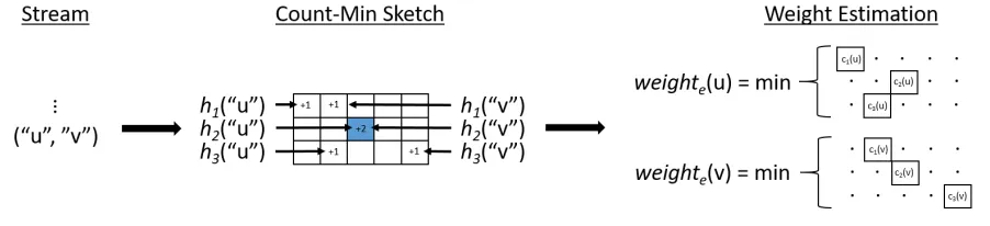
Figure 3.2 How we use a CM sketch for approximating edge weights. . . 42 Figure 3.3 Run times for various approximation parameters compared to the
ex-act implementation. For all approximations, the vertex and edge weight sketches had ε= 10−6 and δ = 10−3. The shared sketch heuristic runs both had a length of l=d e
.0001e. . . 50
Figure 4.1 Example of scoring hyperedges in a stream using hard matching. Hard matching is too constrained for obtaining meaningful results. Even though vertices{1, 3}co-occur inhe1, he2 is given an outlier score of 1. Similarly, he3 is given a score of 1 even though {2, 3} co-occur inhe1. . . 60
Figure 4.2 Example of scoring hyperedges in a stream using soft matching with τ = 0.5. The co-occurrences of vertices is now taken into account, and the hyperedges he2 and he3 are deemed normal. . . 61
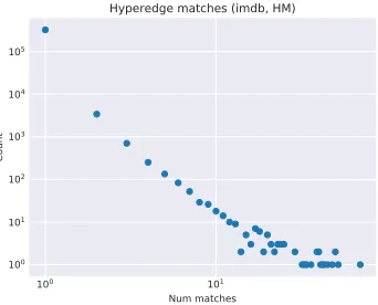
Figure 4.3 How many times each hyperedge is repeated, i.e. it’s count, in the Enron dataset. Figure 4.3a shows hard count, Figure 4.3c shows soft count with τ = 0.25. . . 62 Figure 4.4 Example of computing a single MinHash value for a set. The MinHash
value is the minimum value of the set with respect to the chosen hash function h. . . 63 Figure 4.5 MinHash signatures are formed by kminhash values, each generated by a
different hash function. Signatures are then broken into bbands of length r for storing in the hash tables comprising LSH index. In this figure we show a single hash table for every band, but in reality each band has it’s own hash table. . . 64 Figure 4.6 Average time taken to process “batches” of 1,000 hyperedges. No model
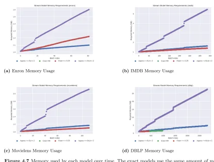
uses batch analysis, times were simply aggregated into batches for illustra-tive purposes. In DBLP the Exact versions were unable to complete in 24 hours, processing less than half the stream. . . 68 Figure 4.7 Memory used by each model over time. The exact models use the same
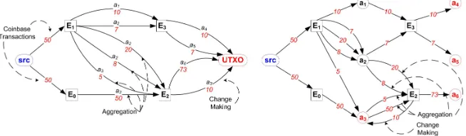
amount of memory, so one time series line is not visible. “Batches” are used for illustrative purposes only, each batch representing the processing of 1,000 hyperedges. . . 70 Figure 5.1 (Left) Bitcoin transactions as a labeled multigraph. (Right) Bitcoin
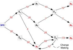
trans-actions as a bipartite multigraph. . . 76 Figure 5.2 Bitcoin transactions as a directed hypergraph. . . 77 Figure 5.3 Graph motifs: (Far Left) The single undirected graph 2-motif (above) with
its three directed motifs α, β, andγ (below), including the two isomorphic α, α0 patterns. (Right) The three undirected 3-motifs and their directed versions. . . 77 Figure 5.4 A 2-motif in a dirhypergraph: Two transactions E1, E2 with sets of tail
and head vertices T1, H1, T2, H2 respectively. (Left) Generic. (Center) A
linear STB. (Right) A circular STB. . . 78 Figure 5.5 (Left) Generic 2-motif. (Right) Instantiated with counts for days 2200-2299
Figure 5.6 Daily activity in each dirhypergraph. . . 81 Figure 5.7 Cumulative percent of addresses with total (left) or average (right) input
and output weights. . . 83 Figure 5.8 Counts (left) and proportions (right) of labeled addresses on the inputs
and outputs of STBs. . . 83 Figure 5.9 Distribution of how many exchange addresses siblings (left) or total siblings
(right) each address has. These distributions were drawn from a random sample of 100K exchanges and 100K non-exchanges. . . 85 Figure B.1 Frequency of exchanges in STBs. . . 113 Figure B.2 Relationship between the number of vertices owned by each exchange and
CHAPTER
1
INTRODUCTION
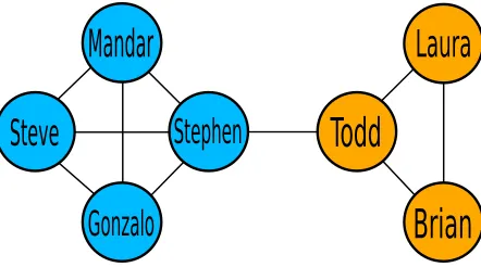
Graphs have gained immense popularity in the research and data science communities, given their ability to represent complex systems and relationships. Each object in the system is a vertex in the graph, and relationships among the objects form theedgesof the graph, connecting vertices. For example, in climate science, regions of the Earth are represented as vertices, and edges connect vertices (regions) which have highly correlated weather variables, such as sea surface temperature. Here edges have a physical interpretation–the correlation between regions of the Earth–but this is not always the case. In social networks, where users are vertices in the graph, edges can represent more abstract relationships, such as friendship, communication, or shared interests. Figure 1.1 shows an example of a co-author graph, where vertices are researchers who have published papers, and two authors share an edge if they have co-published before.
Stephen
Mandar
Steve
Gonzalo
Todd
Laura
Brian
Figure 1.1 Example graph containing two primary groups of co-authors, one group from computer science (blue), and one group from geriatric research (orange). Each author is a vertex, and edges connect authors who have co-published. The bridging edge between Stephen and Todd shows an interesting collaboration between computer science and geriatric research that may warrant further investigation.
entire day, week, or year of activity, many assumptions, such as the graph fitting into memory, or thatO(n2) algorithms will terminate in reasonable time, must be revisited. In this dissertation we focus on developing efficient ways of analyzing large-scale dynamic graphs, with a focus on techniques for anomaly detection. While our specific focus is anomaly detection, we believe the approaches proposed for retaining salient information about the underlying graph is applicable to many other tasks.
Anomaly detection, also referred to as outlier detection, tries to identify data, here graph structures, that are rare, isolated, and/or surprising [11]. For example, edges that act as a “bridge” between groups of vertices often indicate interesting phenomena [5, 58, 139], such as multi-disciplinary collaborations among researchers from otherwise disparate fields, as shown in Figure 1.1. A similar idea has been leveraged to identify unlikely or disallowed paths in system call and program execution graphs, for the purpose of intrusion detection [184]. We focus on developing algorithms for accurate and efficient anomaly detection that directly address two challenges in particular: (1) the increased complexity of the systems being modeled; (2) the growing gap between computing and storage capability, and the volume of data being generated. We address these challenges by designing our algorithms around two cross-cutting ideas. First, we transition from analyzinggraphstreams and series, toedge streams. Second, recognizing that exact analysis is often no longer feasible, we leverage approximation, heuristics, and probabilistic data structures. Specifically, in this dissertation we explore solutions for the following three research objectives.
Figure 1.2 Overview of the main dissertation Chapters, and how they incorporate our solutions to the driving research objectives of efficiency and increased model complexity.
3. Fraudulent pattern mining in the dynamic Bitcoin directed hypergraph (Chapter 5) Figure 1.2 illustrates how each research objective addresses the two cross-cutting challenges outlined above. In Chapter 2 we perform an extensive survey of anomaly detection in dynamic graphs. From this, we identify two important challenges, which lay the foundation for this dissertation. Chapter 3 proposes the first algorithm for outlier detection in graph edge streams. In addition to a fundamentally sound exact model based on link prediction techniques, we show an efficient approximation algorithm that uses probabilistic data structures to provide theoretical error bounds. Similar to Chapter 3, Chapter 4 is the first proposed algorithm for identifying outliers in hyperedge streams. The increased complexity of transitioning from edges to hyperedges necessitates a new form of approximation be used. Finally, Chapter 5 performs a case study on fraudulent pattern mining in the Bitcoin directed hypergraph. Again we increase the complexity, from undirected to directed hypergraphs, but this time rely on heuristics instead of approximation for identifying patterns of interest.
1.1
Graph Based Anomaly Detection
With these advantages, however, come additional challenges. Given such a rich model, it is perhaps obvious that anomalies may be defined in a nearly endless number of ways. Anomalies could be defined at the vertex, edge, or even subgraph level, using topological, attribute, or label information, and be defined locally, e.g. comparing a vertex to its neighbors, or globally, e.g. comparing a vertex to every other vertex in the graph. Moreover, even in plain graphs, which have no attributes or label information on vertices and edges, enumerating the search space is a combinatorially challenging problem. As the substructure(s) of interest grow in complexity, the search space grows superlinearly, in the worst case exponentially.
1.1.1 Anomaly Detection in Dynamic Graphs
In the past decade, focus has shifted from static to dynamic graphs. Unlike static graphs, dynamic graphs allow for modifications to their structure and attributes. For example, in a dynamic graph edges can be inserted or deleted, where a static graph is a snapshot of the system in time, therefore the edge set is fixed. When considering the dynamic nature of the data, new challenges are introduced, such as new types of anomalies, increased storage and processing requirements, and differentiating between organic graph evolution and slow-to-develop anomalies. In Chapter 2 we perform a qualitative comparison and gap analysis of the existing methods. Chapter 2 lays the foundation for the rest of our dissertation, by defining classes of anomalies in dynamic graphs, identifying and mathematically formalizing a two-stage approach that is common among all papers we review, and most importantly identifying open questions and areas of research. The findings of this Chapter were published in [140].
1.1.2 Anomaly Detection in Edge Streams
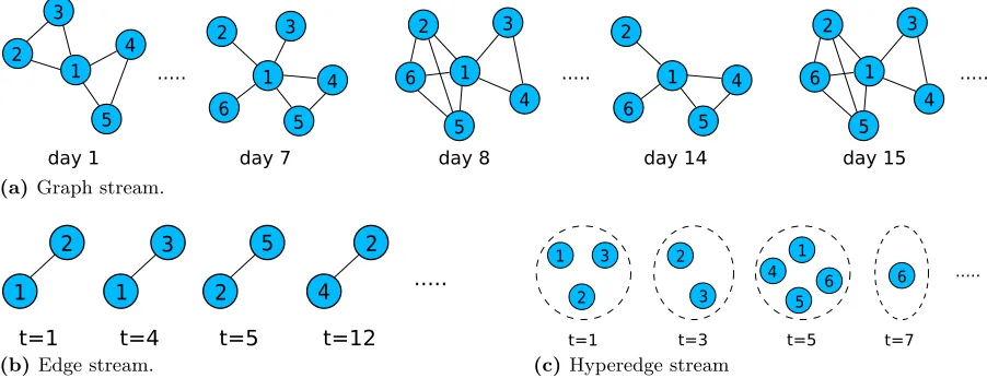
All the methods examined in Chapter 2 represented a dynamic graph using streams or series of graph objects, i.e. each object in the stream was a (static) graph snapshot. Analyzing entire graph snapshots at a time, and comparing adjacent snapshots in the stream, has several drawbacks. First, it requires that entire graphs be stored in main memory for analysis. Second, much or all of the historical information from the stream is lost, as only the most recent snapshots are considered. Third, snapshot comparison often precludes, or severely hinders, the ability to perform fine-grained attribution of detected anomalies. In response to these limitations, we propose a transition from graph stream analysis, to edge streamanalysis, i.e. each object in the stream is a graph edge. Figure 1.3 illustrates the differences between the streaming models discussed.
day 1
...
day 7 day 8
...
day 14 day 15 2 3 1 4 5 1 2 3 4 5 6 1 2 3 4 5 6 1 2 4 5 6 1 2 3 4 5 6 ...
(a) Graph stream.
t=1 t=4 t=5 t=12
... 1 2 1 3 2 5 4 2
(b) Edge stream.
t=1 t=3 t=5 t=7
... 1 2 3 2 3 4 1 6 5 6
(c) Hyperedge stream
Figure 1.3 Each figure shows an example of a different streaming model. Figure (a) shows a graph stream, where each incoming object is an entire graph snapshot, in this example representing a day of activity. Figure (b) shows an edge stream, where each incoming object is an individual graph edge, labeled with the time it was generated. Figure (c) shows a hyperedge stream, where each incoming object is a hyperedge, which may have any positive number of vertices incident on it.
still a challenging problem. We propose a model for calculating an outlier score for each edge in the stream, and utilize Count-Min (CM) sketches to approximate the structural properties of the stream that are relevant to our model. Using CM sketches, we are able to prove theoretical probabilistic error bounds on our edge scores. Results on synthetic and real-world datasets demonstrate empirically the low error rate resulting from approximation, and ability of our method to identify outliers–both quantitatively and qualitatively. All findings from this chapter were published in [139].
1.1.3 Anomaly Detection in Hyperedge Streams
Restricting, or reducing, edges to be pairwise does not faithfully represent numerous types of relationships and interactions, and results in a loss of information. For example, if three researchers co-author a paper together, a graph represents this with three pairwise edges. In Chapter 3 this would result in three new edges in the stream. However, it is possible this same edge configuration may have been the result of every author pair publishing a paper together, and never having published a paper with all three of them. Hyperedges, which can be incident on any positive number of vertices, enable higher order relationships such as these to be captured. In Chapter 4 we propose a method for identifying outliers inhyperedge streams.
combat these challenges. In particular, we use MinHash and locality sensitive hashing (LSH) to facilitate efficient storage and analysis of the stream. Experimental results show that our model is effective in identifying outliers, and support our hypothesis that exact hyperedge matching is too constrained. Moreover, our approximation provides stream processing speedups between 33-750x compared to exact analysis, while maintaining comparable accuracy. The results of this work were published in [141].
1.1.4 Fraudulent Pattern Mining in Directed Hypergraphs
As edges can be directed and undirected in graphs, hyperedges can be directed and undirected in hypergraphs. Directed edges, or arcs, have a single tail vertex and a single head vertex. Directed hyperedges, which we will call hyperarcs from here onward, have a set of tail vertices and a set of head vertices. Directed hypergraphs have been used to model a wide array of domains, from propositional logic [61] to chemical reactions [68]. In Chapter 5 we perform a case study in the Bitcoin network for identifying and reporting potential fraudulent behavior.
Bitcoin is most naturally represented as a directed hypergraph, with each transaction generating a hyperarc in the network. In collaboration with financial forensic experts, we consider what money laundering behavior may look like in the directed hypergraph model. Our analysis focuses on two central topics: exchanges, the entrance and exit from the Bitcoin world; and a specific 2-path pattern we posit could be laundering behavior. Results show we are capable of identifying exchanges in the network with over 80% accuracy using purely structural features of the graph, and that our chosen 2-pattern is exceptionally rare compared to the number of 2-paths in the dirhypergraph. More details can be found in the original publication [142].
1.2
Approximation, Heuristics, and Probabilistic Data
Structures
be leveraged to trade accuracy, precision, or completeness of the solution, with the time and space required to find a solution.
1.2.1 Approximation
We differ in how we use approximation from the conventional use in computer science. Tradi-tionally, approximation refers to algorithms which solve optimization problems, most commonly NP-hard problems, within a provable error bound. A canonical example is a 2-approximation for the minimum vertex cover of a graph, meaning the solution found is guaranteed to be at most twice as large as an optimal solution. On the other hand, when we talk about approximation, we will use it in the context of approximating graph properties or count values. For example, if we want to approximate the degree of a vertex we will try to constrain it to a fixed, known bound. Ifdeg(u) is the true degree of a vertex, we will bound the approximationdege(u) and
use the following notationdeg(u)≤dege(u)≤deg(u) +.
1.2.2 Heuristics
Heuristics are decision making rules chosen for speed, practicality, and intuition, over the global optimality of the choice. While approximation algorithms may employ heuristics, heuristics in general have no requirement to provide error bounds. One of the main heuristics we employ is setting thresholds for labeling outliers. More sophisticated statistical methods, such as auto-regressive moving averages, could be used for calculating outlier threshold values; however, we opt to simply set a threshold value, e.g.score <= 0.05→ outlier.
1.2.3 Probabilistic Data Structures
CHAPTER
2
SURVEY AND ANALYSIS OF ANOMALY
DETECTION IN DYNAMIC GRAPHS
2.1
Introduction
Anomaly detection is an important problem with multiple applications, and thus has been studied for decades in various research domains. In the past decade there has been a growing interest in anomaly detection in data represented as graphs, largely due to their robust expressiveness and their natural ability to represent complex relationships. Examples include global financial systems connecting banks across the world, electric power grids connecting geographically distributed areas, and social networks that connect users, businesses, or customers using relationships such as friendship, collaboration, or transactional interactions. These are examples ofdynamic graphs, which, unlike static graphs, are constantly undergoing changes to their structure or attributes. Possible changes include insertion and deletion of vertices (objects), insertion and deletion of edges (relationships), and modification of attributes (e.g., vertex or edge labels).
events in communication networks [136, 178]; and detecting civil unrest using twitter feeds [39]. The ubiquitousness and importance of anomaly detection in dynamic graphs has led to the emergence of dozens of methods over the last five years (see Tables A.2 and A.3). These methods complement techniques for static graphs [12, 54, 55, 125], as the latter often cannot be easily adopted for dynamic graphs. When considering the dynamic nature of the data, new challenges are introduced, including:
• New types of anomalies are introduced as a result of the graph evolving over time, for example, splitting, disappearing, or flickering communities.
• New graphs or updates that arrive over time need to be stored and analyzed. Storing all the new graphs in their entirety can vastly increase the size of the data. Therefore, typical offline analysis, where multiple passes over the data are acceptable and all of the data are assumed to fit into memory, becomes infeasible. Conversely, storing only the most recent graph or updates restricts the analysis to a single point in time.
• Graphs from different domains, such as social networks compared to gene networks, may exhibit entirely different behavior over time. This divergence in evolution can lead to application-specific anomalies and approaches.
• Anomalies, particularly those that are slow to develop and span multiple time steps, can be hard to differentiate from organic graph evolution.
Although anomaly detection has been surveyed in a variety of domains [23, 34–36, 80], it has only recently been touched upon in the context of dynamic graphs [9, 26, 77]. In this chapter, we hope to bridge the gap between the increasing number of methods for anomaly detection in dynamic graphs and the lack of their comprehensive analysis. In particular, we formalize four types of anomalies in dynamic graphs, develop and fit a taxonomy to all methods analyzed, identify a two-step approach commonly utilized, and qualitatively compare dozens of state-of-the-art methods.
2.2
Background
Table 2.1 Introductory and overview references
Method References
Community detection Fortunato [60], Lancichinetti and Fortunato [100], Reichardt and Bornholdt [144], Harenberg et al. [78]
MDL and Compression Rissanen [147–149], Gr¨unwald [72]
Decomposition Golub and Reinsch [69], Klema and Laub [91], Kolda and Bader [92]
Distance Gao et al. [64], Rahm and Bernstein [137], Cook and Holder [47]
Probabilistic Koller and Friedman [94], Glaz [67]
and well beyond. Cook and Holder [47] show how the theoretical concepts can be applied for graph mining, and Samatova et al. [155] provide an overview of many graph mining techniques as well as implementation details in the R programming language1. For brevity we do not provide an introduction to the fundamentals of the types of methods we discuss, so we provide references for introductory and overview material for each of them in Table 2.1.
It is important to note that in many domains the data are naturally represented as a graph, with the vertices and edges clearly defined. However, in some cases, how to represent the data as a graph is unclear and can depend on the specific research question being asked. The conversion processes used in specific domains are outside the scope of this work, and we assume all data are already represented as dynamic graphs.
Table 2.2 Notation Summary
Symbol Meaning
G Graph series with a fixed number of time points Gt Snapshot of the graph series at timet
Gs The sth graph segment, a grouping of temporally adjacent graphs
It Vertex partitioning at time t, separating all the vertices into disjoint sets
Vt Vertex set for the graph at time pointt
vi Vertexi
Et Edge set for the graph at time pointt
ei,j Edge betweenvi andvj
c0 Threshold value for normal versus anomalous data
1Information on the R programming language can be found at
2.3
Types of anomalies
In this section, we identify and formalize four types of anomalies that arise in dynamic graphs. These categories represent the output of the methods, not the implementation details of how they detect the anomalies, e.g., comparing consecutive time points, using a sliding window technique. Note that often times in real-world graphs (e.g., social and biological networks) the vertex set V is called a set of nodes. However, to avoid confusion with nodes in a physical computer network, and to align with the abstract mathematical representation, we call it a set of vertices.
Because the graphs are assumed to be dynamic, vertices and edges can be inserted or removed at every time step. For the sake of simplicity, we assume that the vertex correspondence and the edge correspondence across different time steps is resolved due to unique labeling of vertices and edges, respectively. We define a graph series G as an ordered set of graphs with a fixed number of time steps. Formally, G = {Gt}Tt=1, where T is the total number of
time steps, Gt = (Vt, Et ⊆(Vt×Vt)), and the vertex setVt and edge set Et may be plain or
attributed (labeled). Graph series where T → ∞ are called graph streams. In the following subsections we start with an intuitive explanation of the problem definition, then give a general formal definition of the anomaly type, continue with some applications, and conclude with a representative example.
2.3.1 Type 1: Anomalous vertices
Anomalous vertex detection aims to find a subset of the vertices such that every vertex in the subset has an “irregular” evolution compared to the other vertices in the graph. Optionally, the time point(s) where the vertices are determined to be anomalous can be identified. What constitutes irregular behavior is dependent on the specific method, but it can be generalized by assuming that each method provides a function that scores each vertex’s behavior, e.g., measuring the change in the degree of a vertex from time step to time step. In static graphs, the single snapshot allows only intra-graph comparisons to be made, such as finding vertices with an abnormal egonet density [12]. Dynamic graphs allow the temporal dynamics of the vertex to be included, introducing new types of anomalies that are not present in static graphs. A high level definition for a set of anomalous vertices is as follows.
Definition 2.1(Anomalous vertices). GivenG, the total vertex setV =ST
t=1Vt, and a specified
scoring function f : V → R, the set of anomalous vertices V0 ⊆ V is a vertex set such that ∀v0∈V0, |f(v0)−fˆ|> c0, where fˆis a summary statistic of the scores f(v), ∀v∈V.
1 2 3 4 5 6 10 9 8 7 1 2 3 4 5 6 10 9 8 7
Time step 1 Time step 2
Community 1
Community 2
Figure 2.1 Example of an anomalous vertex. A dynamic graph with two time steps showing a vertex, v6, that is found to be anomalous based on its change in community involvement. Note that
commu-nities can be overlapping. In time step 1,v6 is only part of community 2, whereas in time step 2 it is
part of both communities 1 and 2. As no other vertexs community involvement changes,v6 is deemed
anomalous.
a substantial change in their community involvement compared to the rest of the vertices in the graph. As v6 is the only vertex that has any change in its community involvement, it is
labeled as an anomaly. Formally, we can measure the change in community involvement between adjacent time stepst andt−1 by lettingf(v) =P|C|
i=1c
t−1
i,v ⊕cti,v, where C={c1, c2, . . . , c|C|} is the set of communities,cti,v = 1 ifv is part of community ci at time steptand 0 otherwise,
and ⊕is the xoroperator.
The scoring functionf will depend on the application. In the example shown in Figure 2.1, the vertices were scored based on the change in community involvement. However, if the objective is identifying computers on a network that become infected and part of a botnet, then an appropriate scoring function might be measuring the change in the number of edges each vertex has between time steps, or the change in the weights of the edges.
Typical applications of this type of anomaly detection are identifying vertices that contribute the most to a discovered event (also known as attribution), such as in communication networks [7], and observing the shifts in community involvement [63, 88].
2.3.2 Type 2: Anomalous edges
abnormal edge weight evolution [105], where the weight of a single edge fluctuates over time and has inconsistent spikes in value, and (ii) appearance of unlikely edges in a graph between two vertices that are not typically connected or part of the same community [1, 143]. Anomalous edge detection can be formally defined as follows.
Definition 2.2 (Anomalous edges). Given G, the total edge set E=ST
t=1Et, and a specified
scoring functionf :E→R, the set of anomalous edgesE0 ⊆E is an edge set such that∀e0 ∈E0,
|f(e0)−fˆ|> c0, where fˆis a summary statistic of the scores f(e), ∀e∈E.
0.45 0.85 0.22 0.45 0.48 0.90 0.77 0.47 0.93 0.87 0.23 0.51 0.47 0.88 0.20
1 1 1 1
2
3
4 2 4 2 4 2 4
3 3 3
t = 1 t = 2 t = 3 t = 4
0.49 0.50
0.91 0.18
1
2 4
3 t = 5 0.50
Figure 2.2 An illustration of anomalous edges that occur because of an irregular pattern of their weight over time, with anomalous edges highlighted. At each time step, a vertex’s weight typically shifts by±0.05 at most. However, edge (3,4) has a spike in its weight at time step 2, unlike any other time in the series. Similarly, at time step 3, edge (1,4) spikes in value. These spikes cause the edges to be considered anomalous
Figure 2.2 shows an example of edges that exhibit irregular edge weight evolutions. Over the five time steps there are two anomalous edges, both having a single time point that is unlike the rest of the series. Letting f(e) =|wt(e)−wt−1(e)|+|wt(e)−wt+1(e)|, where wt(e) is the
edge weight at time step t, each edge is scored based on its current weight compared to the previous and following weight. Abnormally large changes in the weight of an edge results in it being flagged as anomalous. For example, at time step 2, using the mean change in weights
ˆ
f = 0.43 as a summary statistic and c0 = 0.10 as a threshold, results in edge (3, 4) being
declared anomalous.
based on the change in the similarity between itself and every other edge [105].
2.3.3 Type 3: Anomalous subgraphs
Finding subgraphs with irregular behavior requires an approach different from the ones for anomalous vertices or edges, since enumerating every possible subgraph in even a single graph is an intractable problem. Hence, the subgraphs that are tracked or identified are typically constrained, for example, to those found by community detection methods. In these cases, matching algorithms are required to track the subgraphs across time steps, such as the community matching technique used in [70]. Once a set of subgraphs has been determined, intra-graph comparisons or inter-time point comparisons can be made to assign scores to each subgraph, e.g., measuring the change in the total weight of the subgraph between adjacent time steps. Typical intra-graph comparison methods, such as finding unique substructures in the graph that inhibit compressibility [125], must be extended to incorporate the additional information gained by using a dynamic network. Instead of finding structures that are unique withina single graph, structures that are uniqueto a single graphwithin a series of graphs can be found. Anomalies of this type, unique to dynamic networks, include communities that split, merge, disappear and reappear frequently, or exhibit a number of other behaviors.
Definition 2.3 (Anomalous subgraphs). GivenG, a subgraph setH =ST
t=1Ht whereHt⊆Gt,
and a specified scoring functionf :H→R, the set of anomalous subgraphsH0⊆H is a subgraph
set such that ∀h0 ∈ H0, |f(h0)−fˆ| > c
0, where fˆis a summary statistic of the scores f(h), ∀h∈H.
1
2
4
5
6
3
t = 1
1
4
5
3
t = 2
(a) Shrunken Community
1
2
4
5
6
3
t = 1
1
2
4
5
6
3
t = 2
(b) Split Community
Figure 2.3 Two different types of anomalous subgraphs. Figure 2.3a shows a shrunken community, where a community loses members from one time step to the next. Figure 2.3b shows a split commu-nity, where a single community breaks into several distinct smaller communities.
Figure 2.3a, is when a single community loses a significant number of its vertices between time steps. Assuming that a matching of communities between adjacent time stepstandt−1 is known, shrunken communities can be identified by measuring the decrease in the number of vertices in the community, f(h) =|ht∩ht−1| − |ht−1|. Figure 2.3b is an example of asplit community,
when a single community divides into several distinct communities. Split communities will have a high matching score or probability for more than one community in the next graph of the series. Therefore, split communities can be found by examining two adjacent time steps and letting f score each community int−1 as the number of communities it is matched to int.
What constitutes an anomalous subgraph is heavily dependent on the application domain. Automatic identification of accidents in a traffic network can be done by letting edge weights represent outlier scores, then mining the heaviest dynamic subgraph [119]. Similarly, changes and threats in social networks can be found by running community detection on a reduced graph composed of suspected anomalous vertices [82] and performing an eigen decomposition on a residual graph [116].
2.3.4 Type 4: Event and change detection
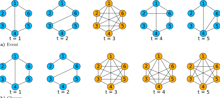
Unlike the previous three types of anomalies, the two types discussed here are exclusively found in dynamic graphs. We start by defining the problem of event detection, which has attracted much interest in the data mining community. Event detection has a much broader scope compared to the previous three types of anomalies, aiming to identify points in time that are significantly different from the rest. Isolated points in time where the graph is unlike the graphs at the previous and following time points represent events. One approach to measuring the similarity of two graphs is comparing the signature vector of summary values extracted from each graph, such as average clustering coefficient. The task of attribution—finding the cause for the event—is not required as part of event detection, and is often omitted. However, once the time points for events have been identified, potential causes can be found by applying techniques for anomaly detection in static graphs [12, 54, 55, 125].
Definition 2.4 (Event detection). Given G and a scoring functionf :Gt→ R, an event is
defined as a time point t, such that|f(Gt)−f(Gt−1)|> c0 and |f(Gt)−f(Gt+1)|> c0.
One of the simplest similarity metrics for graphs is comparing the number of vertices and edges in them. In Figure 2.4a, the event at time step 3 can be found by counting the edges in each graph,f(Gt) =|Et|, and comparing the adjacent time points. The number of edges in each
1 2 4 5 6 3 1 2 4 5 6 3
t = 1 t = 2
1 2 4 5 6 3
t = 3
1 2 4 5 6 3
t = 4
1 2 4 5 6 3
t = 5
(a) Event 1 2 4 5 6 3 1 2 4 5 6 3
t = 1 t = 2
1 2 4 5 6 3
t = 3
1 2 4 5 6 3
t = 4
1 2 4 5 6 3
t = 5
(b) Change
Figure 2.4 Illustration of the difference between an event and change point. An event (Figure 2.4a) is isolated in time, unlike the preceding or subsequent time point. A change point (Figure 2.4b) marks a point in time where the graph undergoes a substantial change, but the change then persists.
Event detection, while providing less specific information than vertex, edge, or subgraph detection, is highly applicable in many areas. Approximating the data available using a tensor decomposition, then scoring the time point as the amount of error in the reconstruction, has been shown to effectively detect moments in time when the collective motions in molecular dynamics simulations change [138]. Other applications include finding frames in a video that are unlike the others [154, 174], and detecting disturbances in the ecosystem (e.g., wildfires) [43].
Now, we move on to the problem of change detection, which is complementary to event detection. It is important to note the distinction between event and change detection. While events represent isolated incidents, change points mark a point in time where the entire behavior of the graph changes, and the difference is maintained until the next change point. Figure 2.4 illustrates the difference between the two. The distinction between events and change points manifests in the modification of the constraint that the value of the scoring function at t be more than a threshold value away from botht−1 andt+ 1, to being more than a threshold value away fromonly t−1.
Definition 2.5 (Change detection). Given Gand a scoring function f :Gt→R, a change is
defined as a time point t, such that|f(Gt)−f(Gt−1)|> c0 and |f(Gt)−f(Gt+1)| ≤c0.
at time step 4, instead of the graph reverting back to its original structure, the added edges are persistent and the graph has a new “normal” behavior. The persistence of the new edges indicates that at t= 3 a change was detected, not an event.
One of the most popular applications of change detection is in networks modeling human interactions, such as communication and co-authorship networks. Authors that act as a “bridge” between different conferences, or switch areas of interest throughout their career, will exhibit a number of change points in their publication records [96]. Additionally, change detection has been applied to communication graphs [7] and network traffic [87] by measuring the change in the eigen decompositions.
2.4
Methods
A common two-stage methodology was found among the papers reviewed. In the first stage, data-specific features are generated by applying a mapping from the domain-specific representation, graphs, to a common data representation, a vector of real numbers. A simple example is taking a single static graph as input and outputting its diameter. In the second stage, an anomaly detector is applied, taking the output from stage one, and optionally some historical data, and mapping it to a decision on the anomalousness of the data. Anomaly detectors, such as support vector machines (SVMs) [167] or the local outlier factor (LOF) algorithm [29], are general methodologies that are domain independent, since they operate on the common data representation that is output from stage one. Hence, stage two consists of identifying outlier points in a multi-dimensional space [4, 13, 14, 29, 133]. The two stages can be formally defined as follows:
Stage one ⇒ Ω :D→Rd
Stage two ⇒ f :{[Rd]∗,[Rd]t} → {0,1}
where D is the domain-specific representation, dis the number of feature dimensions, [Rd]∗
denotes the history of the data, and [Rd]t denotes the current time point. Often times, stage one
maps the domain-specific data to a single value, d= 1, such as the graph diameter example. Additionally, stage two can be generalized to mapping to [0, 1] instead of {0, 1}, representing the probability that the data are anomalous or a normalized outlier score assigned to the data.
are proposing methodologies for stage one, and applying existing methodologies for stage two. A complete list of the methods surveyed is provided in Tables A.2 and A.3.
2.4.1 Community Detection
Community based methods track the evolution of communities and their associated vertices in the graphs over time [168–170]. While the data-specific features generated by the methods discussed in this section are all derived using the community structure of the graphs, the various approaches differ in two main points: (i) in the aspects of the community structure they analyze, e.g., the connectivity within each community vs. how the individual vertices are assigned to the communities at each time step; and (ii) in the definitions of communities they use, e.g., soft communities, where each vertex has a probability of belonging to each community vs. hard, specifically disjoint, communities, where each vertex is placed into at most one community in the graph. Moreover, based on how the community evolution is viewed, it can be applied to the detection of different anomaly types. For example, a rapid expansion or contraction of a community could indicate that the specific subgraph for that community is undergoing drastic changes, whereas a drop in the number of communities by two corresponds to an abnormal event.
2.4.1.1 Vertex detection
Main Idea: A group of vertices that belong to the same community are expected to exhibit similar behavior. Intuitively this means that if at consecutive time steps one vertex in the community
has a significant number of new edges added, the other vertices in the community would also
have a significant number of new edges. If the rest of the vertices in the community did not have new edges added, the vertex that did is anomalous.
Based on this logic, using soft community matching and looking at each community individ-ually, the average change in belongingness (the probability the vertex is part of the community) for each vertex can be found for consecutive time steps. Vertices whose change in belongingness is different from the average change of the vertices in the community are said to beevolutionary community outliers [76].
is anomalous. Later extended to static networks derived from heterogeneous data sources [74], the two step approach in [75] is modified to an alternating iterative approach in [76]. Instead of extracting patterns first and then identifying outliers, the patterns and outliers are found in an alternating fashion (pattern extraction → outlier detection→pattern extraction → · · ·) until the outliers discovered do not change on consecutive iterations. By alternating back and forth between pattern extraction and outlier detection, the algorithm accounts for the affect the outliers have on the communities discovered.
In [88], communities manifest in the form of corenets. Instead of defining the corenet (community) based solely on density, modularity, or hop distance (as egonets are [12]), the definition is based on the weighted paths between vertices. More formally, a vertex’s corenet consists of itself and all the vertices within two hops that have a weighted path above a threshold value. If the edge weight between two vertices is considered the strength of their connection, then intuitively the vertices connected with higher weight edges should be considered part of the same community. Consequently, if a vertex has two neighbors removed, one connected with a high edge weight and the other connected with a low edge weight, then the removal of the vertex connected by the higher edge weight should have more of an impact. At each time step every vertex is first given an outlier score based on the change in its corenet, and the top k outlier scores are then declared anomalous.
2.4.1.2 Subgraph detection
Main Idea: Instead of looking at individual vertices and their community belongingness,
en-tire subgraphs that behave abnormally can be found by observing the behavior of communities themselves over time.
Conversely, instead of finding changes, communities that are conserved, or stable, can be identified. Constructing multiple networks at each time step based on different information sources, communities can be conserved across time and networks. Networks that behave similarly can be grouped using clustering or prior knowledge. In [42], if a community is conserved across time steps and the networks within its group, but has no corresponding community in any other group of networks, then the community is defined as anomalous; two communities are considered corresponding communities if they have a certain percentage of their vertices in common.
Unlike [17, 41, 42] that consider only the structure of the network, in social networks there is often more information available. For example, in the Twitter user network, clusters can be found based on the content of tweets (edges), as well as the users (vertices) involved. If the fraction of the tweets (edges) added during the recent time window for a cluster is much larger than the fraction of tweets (edges) added anytime before the window, then this influx is declared as an evolution event for that cluster [3]. A cluster that experiences an evolution event is marked as an anomalous subgraph at the time when the evolution event occurs. Although the authors did not use labeled datasets in [17], the proposed algorithm can be applied to such data by appropriately incorporating the information in the tensor.
2.4.1.3 Change detection
Main Idea: Changes are detected by partitioning the streaming graphs into coherent segments based on the similarity of their partitionings (communities). The beginning of each segment
represents a detected change.
The segments are found online by comparing the vertex partitioning of the newest graph to the partitioning found for the graphs in the current, growing, segment. Vertex partitioning can be achieved with many methods, but in [53] it is done using the relevance matrix computed by random walks with restarts and modularity maximization. When the partitioning of the new graph is much different from the current segment’s, a new segment begins, and the time point for the new graph is output as a detected change. The similarity of two partitions is computed as their Jaccard coefficient, and the similarity of two partitionings is the normalized sum of their partition similarities. A similar approach, GraphScope [163], based on the same idea but using the MDL principle to guide its partitioning and segmenting will be discussed in the following section.
2.4.2 Compression
done by viewing the adjacency matrix of a graph as a single binary string, flattened in row or column major order. If the rows and columns of the matrix can be rearranged such that the entropy of the binary string representation of the matrix is minimized, then the compression cost (also known as encoding cost [147]) is minimized. The data-specific features are all derived from the encoding cost of the graph or its specific substructures; hence, anomalies are then defined as graphs or substructures (e.g., edges) that inhibit compressibility.
2.4.2.1 Edge detection
Main Idea: An edge is considered anomalous if the compression of a subgraph has higher encoding
cost when the edge is included than when it is omitted.
In [33], a two-step alternating iterative method is used for automatic partitioning of the vertices. Vertex partitioning can be done by rearranging the rows and columns in the adjacency matrix. In the first step, the vertices are separated into a fixed number of disjoint partitions such that the encoding cost is minimized. The second step iteratively splits the partitions with high entropy into two. Any vertex whose removal from the original partition would result in a decrease in entropy is removed from that partition and placed into the new one. Once the method has converged, meaning steps 1 and 2 are unable to find an improvement, the edges can be given outlierness scores. The score for each edge is computed by comparing the encoding cost of the matrix including the edge to the encoding cost if the edge is removed. Streaming updates can be performed using the previous result as a seed for a new run of the algorithm, thus avoiding full recomputations.
2.4.2.2 Change detection
Main Idea: Consecutive time steps that are very similar can be grouped together leading to low compression cost. Increases in the compression cost mean that the new time step differs
significantly from the previous ones, and thus signifies a change.
2.4.3 Matrix/Tensor Decomposition
These techniques represent the set of graphs as a tensor, most easily thought of as a multi-dimensional array, and perform tensor factorization or multi-dimensionality reduction. The most straightforward method for modeling a dynamic graph as a tensor is to create a dimension for each graph aspect of interest, e.g., a dimension for time, source vertices, destination vertices. For example, modeling the Enron email dataset can be done using a 4-mode tensor, with dimensions for sender, recipient, keyword, and date. The element (i, j, k, l) is 1 if there exists an email that is sent from senderito recipient j with keyword k on dayl, otherwise, it is 0.
Similar to compression techniques, decomposition techniques search for patterns or regularity in the data to exploit. All of the data-specific features generated by these methods are derived from the result of the decomposition of a matrix or tensor. Unlike the community methods, these typically take a more global view of the graphs, but are able to incorporate more information (attributes) via additional dimensions in a tensor. One of the most popular methods for matrices (2-mode tensors) is singular value decomposition (SVD) [69], and for higher order tensors (≥ 3 modes) is PARAFAC [79], a generalization of SVD. The main differences among the decomposition based methods are whether they use a matrix or a higher order tensor, how the tensor is constructed (what information is stored), and the method of decomposition.
2.4.3.1 Vertex detection
Main Idea: Matrix decomposition is used to obtain activity vectors per vertex. A vertex is characterized as anomalous if its activity changes significantly between consecutive time steps.
Due to the computational complexity of performing principal component analysis [90] (PCA) on the entire graph, it is computationally advantageous to apply it locally. The approach used in [183] is to have each vertex maintain an edge correlation matrixM, which has one row and column for each of its neighbors. The value of an entry in the matrix for vertexi,Mi(j, k), is
the correlation between the weighted frequencies of the edges (i, j) and (i, k). The weighted frequencies are found using a decay function, where edges that occurred more recently have a higher weight. The largest eigenvalue and its corresponding vector obtained by performing PCA on M are summaries of the activity of the vertex and the correlation of its edges, respectively. The time series formed by finding the changes in these values are used to compute a score for each vertex at each time step. Vertices that have a score above a threshold value are output as anomalies at that time.
2.4.3.2 Event detection
Main Idea: There are two main approaches: (a) Tensor decomposition approximates the original
original data is approximated. Sub-tensors, slices, or individual fibers in the tensor that have
high reconstruction error do not exhibit behavior typical of the surrounding data, and reveal anomalous vertices, subgraphs, or events. (b) Singular values and vectors, as well as eigenvalues
and eigenvectors are tracked over time in order to detect significant changes that showcase
anomalous vertices.
Using the reconstruction error as an indicator for anomalies has been employed for detecting times during molecular dynamics simulations where the collective motions suddenly change [138], finding frames in a video that are unlike the others [174], and identifying data that do not fit any concepts [22].
To address the intermediate blowup problem—when the input tensor and output tensors ex-ceed memory capacity during the computation—Memory-Efficient Tucker (MET) decomposition was proposed [93], based on the original Tucker decomposition [175]. The Tucker decomposition approximates a higher order tensor using a smaller core tensor (thought of as a compressed version of the original tensor) and a matrix for every mode (dimension) of the original tensor. A variety of other tensor decompositions have been developed for offline, dynamic, and streaming analysis [162], in addition to static and sliding window based methods [166]. These extensions allow the method to operate on continuous graph streams as well as those with a fixed number of time points. Compact Matrix Decomposition (CMD) [164] computes a sparse low rank approximation of a given matrix. By applying CMD to every adjacency matrix in the stream, a time series of reconstruction values is created and used for event detection.Colibri[173] and ParCube[131] can be used in the same fashion and provide a large increase in efficiency. The PARAFAC decomposition has been shown to be effective at spotting anomalies in tensors as well [96].
Instead of finding the difference between the graph reconstructed from the approximation obtained by a decomposition, a probabilistic model can be used. The Chung-Lu random graph model [45] is used in [114]. Taking the difference between the real graph’s adjacency matrix and the expected graph’s forms a residual matrix. Anomalous time windows are found by performing SVD on the residual matrices—on which a linear ramp filter has been applied—and by analyzing the change in the top singular values. The responsible vertices are identified via inspection of the right singular vectors. More accurate graph models that also consider attributes are proposed in [115].
projected point outside 3 standard deviations of the rest of the values, and every eigenvector thereafter, constitute the anomalous set. The second step is then to project the data onto its normal and anomalous subspaces. Once this is done, events are detected when the modifications in the anomalous components from the previous time step to the current are above a threshold value [99]. Expanding on this method, joint sparse PCA and graph-guided joint sparse PCA were developed to localize the anomalies and identify the vertices responsible [89]. The responsible vertices are more easily identified by using a sparse set of components for the anomalous set. Vertices are given an anomaly score based on the values of their corresponding row in the abnormal subspace. As a result of the anomalous components being sparse, the vertices that are not anomalous receive a score of 0. Due to the popularity of PCA in traffic anomaly detection, a study was performed identifying and evaluating the main challenges of using PCA [146].
2.4.3.3 Change detection
Main Idea: The activity vector of a graph, u(t), is the principal component, the left singular vector corresponding to the largest singular value obtained by performing SVD on the weighted
adjacency matrix. A change point is when an activity vector is substantially different from the “normal activity” vector, which is derived from previous activity vectors.
The normal activity vector, r(t−1), is the left singular vector obtained by performing SVD on the matrix formed by the activity vectors for the lastW time steps. Each time point is given a scoreZ(t) = 1−r(t−1)|u(t), which is intuitively a score of how different the current activity is compared to normal, where a higher value is worse. Anomalies can be found online using a dynamic thresholding scheme, where time points with a score above the threshold are output as changes [86]. The vertices responsible are found by calculating the ratio of change between the normal and activity vectors. The vertices that correspond to the indexes with the largest change are labeled anomalous. Similar approaches have used the activity vector of a vertex-to-vertex feature correlation matrix [7], and a vertex-to-vertex correlation matrix based on the similarity between vertices neighbors [87].
2.4.4 Distance Measures
2.4.4.1 Edge detection
Main Idea: If the evolution of some edge attribute (e.g., edge weight) differs from the “normal”
evolution, then the corresponding edge is characterized as anomalous.
In [105], a dynamic road traffic network whose edge weights vary over time is studied. The similarity between the edges over time is computed using a decay function that weighs the more recent patterns higher. At each time step, an outlierness score is calculated for each edge based on the sum of the changes in similarity scores. Edges with the highest score, chosen using either a threshold value or top-kheuristic, are marked as anomalous at that time step.
Viewing each individual network in the sequence as a timestamped stream of edges, meaning the network does not have a fixed topology as the road traffic network did, the frequency and persistence of an edge can be measured and used as an indicator of its novelty. The persistence of an edge is how long it remains in the graph once it is added, and the frequency is how often it appears. In [1], set system discrepancy [38] is used to measure the persistence and frequency of the edges. When an edge arrives, its discrepancy is calculated and compared to the mean discrepancy value of the active edge set. If the weighted discrepancy of the edge is more than a threshold level greater than the mean discrepancy, the edge is declared novel (anomalous). Using the novel edges detected, a number of metrics can be calculated for various graph elements (e.g., vertices, edges, subgraphs). Individual graph elements can then be identified anomalous via comparison of the calculated metrics for that element with the overall distribution and change of the metric.
2.4.4.2 Subgraph detection
Main Idea: A subgraph with many “anomalous” edges is deemed anomalous.
a solution to the NP-hard problem. This work was later extended to allow the subgraphs to smoothly evolve over time, where vertices can be added or removed between adjacent time steps [118]. A similar approach mines weighted frequent subgraphs in network traffic, where the edge weights correspond to the anomaly contribution of that edge [81].
2.4.4.3 Event detection
Main Idea: Provided a function f(Gi, Gj) that measures the distance between two graphs, a time
series of distance values can be constructed by applying the function on consecutive time steps
in the series. Anomalous values can then be extracted from this time series using a number of
different heuristics, such as selecting the top kor using a moving average threshold.
Extracting features from the graphs is a common technique to create a summary of the graph in a few scalar values, its signature. Local features are specific to a single vertex and its egonet [12] (the subgraph induced by itself and its one-hop neighbors), such as the vertex or egonet degree.Global features are derived from the graph as a whole, such as the graph radius. The local features of every vertex in the graph can be agglomerated into a single vector, the signature vector, of values that describe the graph using the moments of distribution (such as mean and standard deviation) of the feature values. In [25], the similarity between two graphs is the Canberra distance, a weighted version of theL1 distance, between the two signature vectors.
A similar approach is used in [101] to detect abnormal times in traffic dispersion graphs. Instead of an agglomeration of local features, it extracts global features from each graph, introducing a dK-2 series [109, 153, 179] based distance metric, and any graph with a feature value above a threshold is anomalous.
As an alternative to extracting multiple features from the graph and using the signatures, the pairwise vertex affinity scores may be used. Pairwise vertex affinity scores are a measure of how much each vertex influences another vertex, and can be found using fast belief propagation [97]. In [58] the scores are calculated for two consecutive time steps, and the similarity between the two graphs is the rooted Euclidean distance (Matusita distance) between the score matrices. The changes in the vertex affinity score are shown to accurately reflect and scale with the level of impact of the changes. For example, removing an edge that connects two otherwise disconnected components, a “bridging edge,” results in a higher score than removing an edge that does not affect the overall structure of the graph. A moving threshold is set on the time series of similarity scores using quality control with individual moving range. The exponential weighted moving average has also been used as a way to dynamically set the threshold, tested on distribution features extracted from Wikipedia revision logs [16].