Analysis of Numerical Dispersion in the High-Order
2-D WLP-FDTD Method
Wei-Jun Chen1, *, Jun Quan2, and Shi-Yu Long1
Abstract—A theoretical analysis of numerical dispersion in the high-order finite-difference time-domain (FDTD) method with weighted Laguerre polynomials (WLPs) is proposed in this paper. According to the numerical dispersion relation for the two-dimensional (2-D) case, the numerical phase velocities relevant to the direction of wave propagation, grid discretization and time-scale factor are obtained. For a fixed relative error of the numerical phase velocity, the suitable sampling point density and time-scale factor can be determined. Compared with the low-order WLP-FDTD, the high-order one shows its good dispersion characteristics while a low sampling density is used. Three numerical examples are included to validate the effectiveness of the high-order scheme.
1. INTRODUCTION
The finite-difference time-domain (FDTD) method is a very popular time-domain method for solving electromagnetic problems, but its time step is constrained by the Courant-Friedrich-Levy (CFL) stability condition [1]. To overcome this limitation, an unconditionally stable FDTD method, which combines weighted Laguerre polynomials (WLPs) as the basis function with Galerkin’s testing procedure, was proposed by Chung et al. [2]. For some problems with fine structures, this method shows much better efficiency than the conventional FDTD method.
Generally, WLP-FDTD results in a huge sparse matrix equation, which is challenging to solve. In [3–6], the factorization-splitting techniques were proposed to divide the huge matrix into small ones corresponding to different electromagnetic components. Based on the solution of the Schur complement system, a domain decomposition scheme is implemented in WLP-FDTD to improve the efficiency [7]. To reduce the number of unknowns in the huge matrix, scaling functions [8] and mixed-order scheme [9] are introduced into WLP-FDTD to decrease the sampling density in space domain, respectively. Thus, the produced sparse matrix with a much smaller number of unknowns leads to a more efficient solution of WLP-FDTD.
For the fourth-order WLP-FDTD method, an analysis of numerical dispersion for the two-dimensional (2-D) case is presented in this paper. Besides the direction of wave propagation and grid discretization, the time-scale factor s is necessarily involved and influences the dispersion errors to a great degree. From its numerical dispersion relation, small relative errors of the numerical phase velocity can be obtained while the low sampling density is used. Three numerical examples are tested to show the necessity of numerical dispersion analysis in the high-order scheme.
Received 12 May 2015, Accepted 31 July 2015, Scheduled 12 August 2015
* Corresponding author: Wei-Jun Chen (chenw [email protected]).
1 School of Information Science and Technology, Lingnan Normal University, Zhanjiang 524048, China. 2 School of Physics Science
2. NUMERICAL DISPERSION ANALYSIS
The time-domain Maxwell’s equations for a 2-D TEz wave propagating in free space can be written as
ε0∂Ex|x,y,t
∂t =
∂Hz|x,y,t
∂y , (1a)
ε0∂Ey|x,y,t
∂t =−
∂Hz|x,y,t
∂x , (1b)
μ0∂Hz|x,y,t
∂t =
∂Ex|x,y,t
∂y −
∂Ey|x,y,t
∂x , (1c)
whereε0andμ0are the electric permittivity and magnetic permeability of free space, respectively. With
reference to [2], the 2-D implicit formulation for WLP-FDTD can be given by introducing the Laguerre basis functions and Galerkin’s testing procedure
Exp|x,y =
2 sε0
∂Hzp|x,y
∂y −2
p−1
q=0, p>0
Exq|x,y, (2a)
Eyp|x,y =−
2 sε0
∂Hzp|x,y
∂x −2
p−1
q=0, p>0
Eyq|x,y, (2b)
Hzp|x,y =
2 sμ0
∂Exp|x,y
∂y −
2 sμ0
∂Eyp|x,y
∂x −2
p−1
q=0, p>0
Hzq|x,y, (2c)
where s is the time-scale factor andp is the order of Laguerre functions. For a monochromatic wave, Exp,Eyp and Hzp are expanded into a discrete set of Fourier modes as follows [6, 10]:
Exp|i,j , Eyp|i,j , Hzp|i,j
=Exp, Eyp, Hzpej0(ikΔxcosϕ+jkΔysinϕ), (3)
where (i, j) denotes the spatial index of a field component, Δx and Δy are the space steps along the x- and y-axes, j0 =
√
−1,k is the wavenumber, and ϕis the angle between the propagation direction and x-axis. The fourth-order central-difference formula for staggered grids can be written as [11]
df(x)
dx =
9 8
f(x+ 0.5Δx)−f(x−0.5Δx)
Δx −
1 24
f(x+ 1.5Δx)−f(x−1.5Δx)
Δx . (4)
Inserting (3) and (4) into (2), we get
Exp− H
p z
27ej0b−e−j0b−ej03b−e−j03b
12sε0Δy
=−2
p−1
q=0, p>0
Exq, (5a)
Eyp+ H
p z
27ej0a−e−j0a−ej03a−e−j03a
12sε0Δx
=−2
p−1
q=0, p>0
Eyq, (5b)
27ej0b−e−j0b−ej03b−e−j03b
−12sμ0Δy E
p x+
27ej0a−e−j0a−ej03a−e−j03a
12sμ0Δx E
p
y +Hzp=−2 p−1
q=0, p>0
Hzq (5c)
where a = 0.5kΔxcosϕ and b = 0.5kΔysinϕ. Using Euler’s formula, (5) can be written in a matrix form as
AEp=
p−1
q=0,p>0
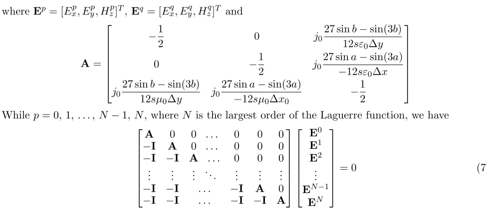
whereEp= [Exp, Eyp, Hzp]T,Eq= [Exq, Eyq, Hzq]T and A= ⎡ ⎢ ⎢ ⎢ ⎢ ⎢ ⎢ ⎣ −1
2 0 j0
27 sinb−sin(3b) 12sε0Δy
0 −1
2 j0
27 sina−sin(3a) −12sε0Δx
j0
27 sinb−sin(3b) 12sμ0Δy j0
27 sina−sin(3a)
−12sμ0Δx0 −
1 2 ⎤ ⎥ ⎥ ⎥ ⎥ ⎥ ⎥ ⎦
While p= 0,1, . . . , N −1, N, whereN is the largest order of the Laguerre function, we have ⎡ ⎢ ⎢ ⎢ ⎢ ⎢ ⎢ ⎣
A 0 0 . . . 0 0 0
−I A 0 . . . 0 0 0
−I −I A . . . 0 0 0 ..
. ... ... . .. ... ... ... −I −I . . . −I A 0 −I −I . . . −I −I A
⎤ ⎥ ⎥ ⎥ ⎥ ⎥ ⎥ ⎦ ⎡ ⎢ ⎢ ⎢ ⎢ ⎢ ⎢ ⎣ E0 E1 E2 .. .
EN−1 EN ⎤ ⎥ ⎥ ⎥ ⎥ ⎥ ⎥ ⎦
= 0 (7)
whereIis a 3×3 identity matrix. For a nontrivial solution of homogeneous Equation (7), the determinant of its coefficient matrix should be zero, thus leading to |A|N+1 = 0. Consequently, it can be derived
729 sin2b
Δy2 +
sin2(3b) Δy2 −
54 sinbsin(3b)
Δy2 +
729 sin2a
Δx2 +
sin2(3a)
Δx2 −
54 sinasin(3a)
Δx2 =−
144s2ε0μ0
4 . (8)
When Δx= Δy→0 in (8), the theoretical solution of the time-scale factor can be expressed as s0=|Im(s)|=
2k √
ε0μ0
= 4πf0, (9)
wheref0 is the operating frequency. It can be seen from (8) that the numerical dispersion of high-order
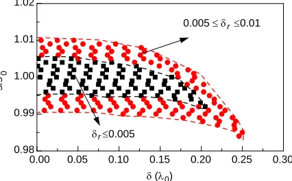
WLP-FDTD relates to the propagation direction, sampling density in space domain and time-scale factor. The relative error of the numerical phase velocity is:
δr =
νp−c
c = 1 24πδ s0 s ⎡ ⎢ ⎢ ⎢ ⎣
729 sin2(πδsinϕ) + sin2(3πδsinϕ) −54 sin(πδsinϕ) sin(3πδsinϕ)+ 729 sin2(πδcosϕ) + sin2(3πδcosϕ) −54 sin(πδcosϕ) sin(3πδcosϕ)
⎤ ⎥ ⎥ ⎥ ⎦−1
, (10)
wherevp is the numerical phase velocity, c= 1/√ε0μ0 is the speed of light in free space,δ = Δx/λ0 =
Δy/λ0 andλ0 is the operating wavelength.
Figure 1 plots two regions that denote two different intended error ranges, δr ≤ 0.005 and
0.005 < δr ≤ 0.01. Here, the errors are the maximum ones for ϕ ∈ [0◦,90◦] in (10). If the value
of an intended error is given, it is easy to determine the suitable combinations of sand δ.
Figure 2(a) plots the curves which illustrate the variation of vp with propagation angle ϕ. Here,
three different sampling densities with three different values ofs/s0 are examined. For comparison, the
variation in the low-order method is also calculated in Figure 2(b). vp is dependent upon the direction
of wave propagation and it is maximum for waves propagating obliquely with the grid (ϕ = 45◦). To obtain acceptable numerical dispersion errors, fewer grid cells per wavelength are required than those in low-order WLP-FDTD. It is noteworthy from Figure 2 that the value of the time-scale factor salso determines the numerical error. Whens0/s= 1,vp is much closer to the speed of light cthan the other
cases.
3. NUMERICAL RESULTS
Table 1. Comparison between different time-scale factors.
TE10 TE20
Solution (MHz) Error (%) Solution (MHz) Error (%)
Analytic 124.94 - 249.89
-0.98s0 125.06 0.096 248.98 0.37
0.99s0 125.01 0.054 248.98 0.37
s0 125.01 0.054 249.13 0.30
1.01s0 124.96 0.013 249.05 0.33
1.02s0 125.03 0.075 249.03 0.34
is used as the incident electric current profile:
Jx(t) = exp
−
t−Tc
Td
2
sin [2πfc(t−Tc)], (11)
where Td = 1/(2fc), Tc = 6Td and fc = 0.2 GHz. And we choose the time duration Tf = 160 ns. This
duration is chosen in such a way that the waveforms of interest have practically decayed to zero [2]. Assuming the maximum operating frequencyfmax= 520 MHz, we can obtain s= 6.5345×10⁹ with (9)
and N = 272 from [10]. In this example, uniform square cells with Δx = Δy = 0.1 m (about six cells per λ, where λis the wavelength corresponding tofmax) are used to divide the 2-D space domain.
By performing the fast Fourier transform (FFT) to the time-domain data from the high-order WLP-FDTD with different time-scale factor s, we can obtain the first two cutoff frequencies and the relative error, results as shown in Table 1. From Table 1, it is seen that the relative errors are all very small (<0.1%) for TE10 mode. And the error is the smallest while the time-scale factor sis chosen as
the theoretical solution s0 for TE20 mode.
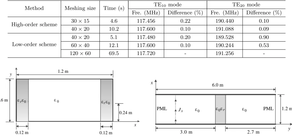
As the second example, the cutoff frequencies of the first two modes in a 2-D partially loaded rectangular waveguide, shown in Figure 3, are calculated. Since the geometry is uniform in the y direction, the TE10 and TE20 modes have no y dependence [12]. The same modulated Gaussian pulse
and parameters as the first example are used.
Table 2 shows the computational efforts and results with the high-order and low-order WLP-FDTD methods for different grid divisions. Considering the low-order WLP-FDTD method with the fine mesh (120×60) as the benchmark, the high-order scheme shows its accurate results when occupying smaller meshing size and less CPU time.
The third example is to calculate the reflected signal power in a 2-D parallel plate waveguide with a thin dielectric interface, shown in Figure 4. The same modulated Gaussian pulse as (11) is used as x-direction input current profile with fc = 0.4 GHz. And we choose the time duration Tf = 80 ns.
0.00 0.05 0.10 0.15 0.20 0.25 0.30
0.98 0.99 1.00 1.01 1.02
s
/s0
r 0.005 ≤ δ ≤0.01
r δ ≤0.005
δ (λ 0)
0 45 90 0.90
0.92 0.94 0.96 0.98 1.00
1.02 20 cell/λ
10 cell/λ
s/s =0.990
s/s =10
s/s =1.010
5 cell/λ
p
c
0 15 30 45 60 75 90
0.985 0.990 0.995 1.000 1.005 1.010
6 cell/λ
8 cell/λ
10 cell/λ
p
c
0
s s =1.01
(b) (a)
ϕ (degrees) ϕ (degrees)
s/s =0.990
s/s =0.990
ν ν
Figure 2. Variation of numerical phase velocity with the propagation angle, sampling density and time-scale factor in (a) high-order and (b) low-order method.
Table 2. Comprison between high- and low-order schemes.
Method Meshing size Time (s) TE10 mode TE20 mode
Fre. (MHz) Difference (%) Fre. (MHz) Difference (%)
High-order scheme 30×15 4.6 117.456 0.22 190.440 0.10
40×20 10.2 117.600 0.10 191.088 0.09
Low-order scheme
40×20 5.1 117.480 0.20 189.528 0.90
60×40 12.1 117.600 0.10 190.244 0.53
120×60 69.5 117.720 - 191.256
-0.6 m
0.24 m 1.2 m
0.12 m 0.12 m
ε εr 0 ε εr 0
x y
ε0
Figure 3. Cross-section of a 2-D waveguide loaded with a dielectric block of εr = 9.
1.2 m
x 6.0 m
3.0 m 2.7 m
Jx
PML PML
y ε ε0 r ε0
ε0
Figure 4. 2-D parallel plate waveguide with a thin dielectric interface of εr = 9.
Assuming the maximum operating frequencyfmax= 1 GHz, we can obtains= 1.2566×10¹⁰with (9) and
N = 261 from [10]. A perfectly matched layer (PML) with 2nd-order central-difference as the absorbing boundary condition is used to truncate the open areas [9]. In this example, the PML includes‘8 layers with quadratic polynomial increase of conductivity of 0.1% theoretical reflection coefficients at normal incidence.
From the calculated temporal electric fields, the reflected signal powers are obtained through discrete Fourier transform (DFT). Figure 5 shows that the reflected signal powers from the high-order and low-high-order WLP-FDTDs with different grid discretization. Table 3 shows the requirement of CPU time and memory. Considering the low-order method with the grid discretization of 15 cell/λ (λ is the wavelength corresponding to fmax) as the benchmark, the difference from the high-order
0.53 0.54 0.55 0.56
Freq. (MHz)
High-order (8 cell/λ)
High-order (10 cell/λ)
Low-order (15 cell/λ) -60
-40 -20 0
Reflected signal power (dB)
Figure 5. Reflected signal power calculated with high- and low-order WLP-FDTDs.
Table 3. Comparison between Different Methods.
Method Meshing size Memory (MB) CPU time (s) Difference (%)
High-order (8 cell/λ) 160×32 5.15 64 0.87
High-order (10 cell/λ) 200×40 7.23 97 0.037
Low-order (15 cell/λ) 300×60 11.7 126
-requirement are needed with the accepted numerical difference. The difference are calculated by the formula: (PminH−O−PminB−M)/PminB−M ×100%, where PminH−O, PminB−M index the minimum reflected signal
power for high order and the benchmark, respectively. The value of relative permeability is equal to 1. All calculations have been performed on an AMD Phenom II×6 2.80 GHz machine with 8 GB RAM.
4. CONCLUSION
In this paper, with the fourth-order central difference in space domain, the numerical dispersion of high-order 2-D WLP-FDTD is analyzed. Its dispersion relation is associated with the propagation direction, sampling density in space domain and time-scale factor. Different from the conventional FDTD, the suitable selection of the time-scale factor leads to low numerical dispersion errors. Furthermore, compared with low-order WLP-FDTD, good dispersion characteristic can be observed with the low sampling density.
ACKNOWLEDGMENT
We gratefully acknowledge support by the National Natural Science Foundation of China (Grant No. 11304276), the Natural Science Foundation of Guangdong Province, China (Grant No. 2014A030307035).
REFERENCES
1. Taflove, A. and S. C. Hagness,Computational Electrodynamics: The Finite-difference Time-domain
Method, Artech House, Boston, MA, 2005.
2. Chung, Y. S., T. K. Sarkar, B. H. Jung, and M. Salazar-Palma, “An unconditionally stable scheme for the finite-difference time-domain method,”IEEE Trans. on Microwave Theory and Technique, Vol. 51, No. 3, 697–704, 2003.
4. Duan, Y. T., B. Chen, D.-G. Fang, and B.-H. Zhou, “Efficient implementation for 3-D Laguerre-based finite-difference time-domain method,” IEEE Trans. on Microwave Theory and Technique, Vol. 59, No. 1, 56–64, Jan. 2011
5. Chen, Z., Y. T. Duan, Y. R. Zhang, and Y. Yi, “A new efficient algorithm for the unconditionally stable 2-D WLP-FDTD method,” IEEE Trans. Antennas Propag., Vol. 61, No. 7, 3712–3720, Jul. 2013.
6. Chen, Z., Y. T. Duan, Y. R. Zhang, H.-L. Chen, and Y. Yi, “A new efficient algorithm for 3-D Laguerre-based finite-difference time-domain method,” IEEE Trans. Antennas Propag., Vol. 62, No. 4, 2158–2164, Apr. 2014.
7. He, G.-Q., W. Shao, X.-H. Wang, and B.-Z. Wang, “An efficient domain decomposition Laguerre-FDTD method for two-dimensional scattering problems,” IEEE Trans. Antennas Propag., Vol. 61, No. 5, 2639–2645, May 2013.
8. Alighanbari, A. and C. D. Sarris, “An unconditionally stable Laguerre-based S-MRTD time-domain scheme,” IEEE Antennas Wireless Propag. Lett., Vol. 5, 69–72, 2006.
9. Profy, F. and Z. Chen, “Efficient mixed-order FDTD using the Laguerre polynomials on non-uniform meshes,” IEEE/MTT-S International Microwave Symposium, 1967–1970, Jun. 2007. 10. Chen, W.-J., W. Shao, J.-L. Li, and B.-Z. Wang, “Numerical dispersion analysis and key parameter
selection in Laguerre-FDTD method,”IEEE Microw. Wireless Compon. Lett., Vol. 23, No. 12, 629– 631, Dec. 2013.
11. Gustafsson, B., High Order Difference Methods for Time Dependent PDE, Springer, Berlin, Heidelberg, 2008