Deployment of a Matrix Element Method code for the ttH channel analysis on GPU’s platform

Deployment of a Matrix Element Method code for the ttH

channel analysis on GPU’s platform

GillesGrasseau1,∗_{,FlorianBeaudette}1,∗∗_{,CristinaMartin Perez}1,∗∗∗_{,AlexandreZabi}1,∗∗∗∗_, ArnaudChiron1,†_{,ThomasStrebler}2,‡_{, andGabrielHautreux}3,§

1_{Laboratoire Leprince-Ringuet, Ecole polytechnique, Palaiseau, France}

2_{Laboratoire Leprince-Ringuet, Ecole polytechnique, Palaiseau, France. Now at Centre de Physique} des Particules de Marseille, Aix-Marseille Université, CNRS/IN2P3, Marseille, France

3_{GENCI “Grand Equipement de Calcul Intensif”, 6 bis rue Auguste Vitu, Paris, France}

Abstract.The observation of the associated production of the Higgs boson with two top quarks in proton-proton collisions is one of the highlights of the LHC Run 2. Driven by the theoretical description of the physics processes, the Ma-trix Element Method (MEM) consists in computing a probability that an event is compatible with the signal hypothesis (ttH) or with one of the background hypotheses. It is a powerful classifying tool requiring high dimensional integral computations. The deployment of our MEM production code on GPU’s plat-form will be described. What follows will focus on the adaptation of the main components of the computations in OpenCL kernels, namely the Magraph ma-trix element code generator, VEGAS, and LHAPDF. Finally, the gain obtained on GPU’s platforms compared with classicalCPU’s platforms will be assessed.

1 Introduction

The recent observation of the associated production of the Higgs boson with two top quarks [1] is one of the highlights of the Run 2 at the LHC. Since its observation in 2012 [2, 3], the properties of the new Higgs boson have been extensively tested, and in particular, its couplings to other particles. In the Standard Model, the fermions couple to the Higgs boson through a Yukawa interaction with a strength proportional to the fermion mass. Consequently, the coupling of the Higgs boson to thebandτlight fermions have been inferred from the

decay rate of the Higgs boson inbb[4] andττ[5] respectively. However, this strategy does not apply to the coupling with the top quark,yt, as the decay of the Higgs boson into a top

quark pair is kinematically forbidden. Instead, theytcoupling can directly be measured from

the rare associatedttHproduction process.

The combination of Run 1 and 2016 Run 2 data from LHC collisions allowed the first observation[1] of the simultaneous production of a Higgs boson with att¯pair in April 2018.

∗_{e-mail: [email protected]} ∗∗_{e-mail: [email protected]} ∗∗∗_{e-mail: [email protected]} ∗∗∗∗_{e-mail: [email protected]}

†_{e-mail: [email protected]} ‡_{e-mail: [email protected]} §_{e-mail: [email protected]}

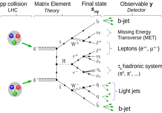
Figure 1.ttHproduction process: (Left) Feynman diagrams of the Higgs boson production in associa-tion with top quarks, resulting from top quark fusion (top) or Higgs radiaassocia-tion from a top quark (bottom); (Right) an event candidate for the production of a top quark and top anti-quark pair in addition with a Higgs Boson in the CMS detector[6].

2 The Matrix Element Method

Unlike supervised methods (neural networks, decision trees, support vector machines, ...), the Matrix Element Method[7] allows events to be classified by computing the probability that a final state corresponds to a given physics process solely thanks to the physics laws involved. Among the new emerging computing models based on Machine or Deep Learning, it is essential to have a theory-driven model which plays the role of computational reference. This sophisticated method is however veryCPUtime consuming due to the investigation of all the main physical cases and requires huge powerful computing platforms to perform the CMS analyses carried out at our laboratory in a reasonable time. Thanks to the pioneering works of [9, 10] on the implementation of the MEM on a single GPU, we were confident that the multi-GPU implementation was achievable.

2.1 Principle

Given the various possible decay channels of Higgs boson and of theW resulting from the t→Wb decay, thettH signal can result in a large variety of final states. In the analysis considered here, one of theWbosons is required to decay leptonically and the Higgs boson is required to decay intoτ+_τ−_{(Fig. 2). This final state offers a good compromise between the}

total branching ratio and the purity. To further reduce the background, the charged leptons produced in theτandWdecay are required to have the same electric charge.

For each event of the data set to analyze, the probabilities or weights are evaluated for a given theory model (signalorbackground). This probability expression is shown below. An integration is performed over all the possible values of the generator-level variables x

and the Bjorken fractions of the incoming partonsxa andxb. The response of the detectors

Figure 1.ttHproduction process: (Left) Feynman diagrams of the Higgs boson production in associa-tion with top quarks, resulting from top quark fusion (top) or Higgs radiaassocia-tion from a top quark (bottom); (Right) an event candidate for the production of a top quark and top anti-quark pair in addition with a Higgs Boson in the CMS detector[6].

2 The Matrix Element Method

Unlike supervised methods (neural networks, decision trees, support vector machines, ...), the Matrix Element Method[7] allows events to be classified by computing the probability that a final state corresponds to a given physics process solely thanks to the physics laws involved. Among the new emerging computing models based on Machine or Deep Learning, it is essential to have a theory-driven model which plays the role of computational reference. This sophisticated method is however veryCPUtime consuming due to the investigation of all the main physical cases and requires huge powerful computing platforms to perform the CMS analyses carried out at our laboratory in a reasonable time. Thanks to the pioneering works of [9, 10] on the implementation of the MEM on a single GPU, we were confident that the multi-GPU implementation was achievable.

2.1 Principle

Given the various possible decay channels of Higgs boson and of theW resulting from the t→Wb decay, thettH signal can result in a large variety of final states. In the analysis considered here, one of theW bosons is required to decay leptonically and the Higgs boson is required to decay intoτ+_τ−_{(Fig. 2). This final state offers a good compromise between the}

total branching ratio and the purity. To further reduce the background, the charged leptons produced in theτandWdecay are required to have the same electric charge.

For each event of the data set to analyze, the probabilities or weights are evaluated for a given theory model (signalorbackground). This probability expression is shown below. An integration is performed over all the possible values of the generator-level variables x

and the Bjorken fractions of the incoming partonsxaandxb. The response of the detectors

is modelled through Transfer Functions (TF). In particular, gaussian response functions turn out to be very well adapted to mimick the jet response, as well as the missing transverse momentum (x,y) components. For the tau leptons, the semi-analytic TF have been used.

They predominantly account for the emissions of neutrino(s) and therefore depend on the tau decay channel.

wi(y)= 1 σi

p

dxdxadxbf(xa,Q).f(xb,Q)

xaxbS δ 4_(x

aPa+xbPb−ΣPk)|Mi(x)|2W(y||x) (1)

This probabilitywi(y) sums all possible contributions of the matrix element|Mi(x)|2

(eval-uated in the rest frame of the outgoing particles) for a processiand is convolved by the Trans-fer FunctionW(y_||x), the probability to have the observed state described by the variablesy, given the kinematic variablesx. A second ponderation f(xa,Q).f(xb,Q)

xaxbS gives the probability that

the two incoming proton particles or partons (proton quarks or gluons) interact, in which f(xa,Q) is the Parton Density Function (or PDF) for the partona. All the parton

combi-nations are described by theΣpterm. Finally, theδ4(xaPa+xbPb−ΣPk) term corresponds

to the kinematic constraints between the p-p incoming partons and the outgoing particles considered in the Matrix Element.

Figure 2. The final state considered in our analysis: bb¯, qq¯ pairs, τh, 2 same sign leptons and 3

undetectable neutrinosνs. Theτ−decays in a hadronic system referred to asτh is constituted by

pions particlesπ±_(π0₎n_{, π}±_π∓_π± _{. . . together with aν}

τ neutrino. The CMS reconstruction software,

CMSSW, reconstructs the jets, identifies theband light quarks, the hadronicτh, leptons and the Missing

Transverse Energy (MET) collecting the transverse energy of undetectable neutrinos.

2.2 Background processes

The same final state can be obtained from several background processes and only the domi-nant ones are considered for the matrix element computations. For the irreduciblettZ back-ground where theHboson of the signal is simply replaced by aZboson, the MEM computa-tion is the same as with the signal, except for the matrix element component of the integral. For the reducible backgrounds, (ttZ,Z→ll) andtt, where one of the objects is mis-identified,¯ the matrix element and the Transfer Functions as well as the integration strategies are modi-fied.

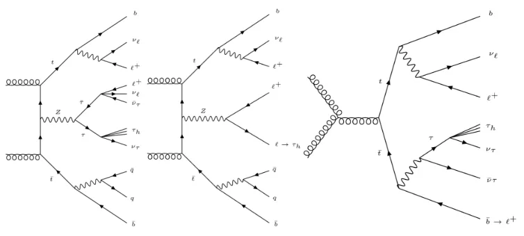
Figure 3.Mainbackgroundprocesses leading to the observation of the same final state. (Left)ttZ,Z→ττ, theZboson replaces the Higgs boson in this diagram.

(Middle)ttZ,Z → ll, with one of the leptons misidentifed, in this case theZ boson decays in two leptons, and one them is misidentified by the reconstruction software and associated with an hadronic tau particleτh.

(Right)tt¯, with an additional lepton produced in the decay of Bhadrons. Additional light jets can be produced due to some QCD radiation, leading to the final state observation, but are not taken into account in the matrix element.

2.3 Permutations and integration multiplicity

Up to now, we have seen that we have to compute 4 integrals per event: 1 to compute the probability that belongs to the signal class and 3 to belong each of the considered background classes. However, we have to consider that an observed b-jet can be assigned to thebquark or the ¯bof thettHprocess. Similarly, several different configurations give rise to two same-sign

leptons: their observations in the detector cannot be assigned uniquely to the one coming from theτ+_{decay and the other coming from theW}+_{decay. As a result, we have to take into} account the 4 lepton-bottom permutations for each of the 4 signal/background probabilities

to compute. Besides, the possibility that a jet falls out of the detector acceptance is also taken into account and requires a specific integration.

There is another multiplicative factor that increases the number of integrals to compute. It occurs for events in which only one quark has been identified, leading to a missingqq¯pair in the final state. In this special case, integrals are computed by assigning a light-jet from the light jet list identified in the event to the missing quark of the final state. For this kind of event, 4×4×nlight−jetsintegrals, wherenlight−jets is the number of light-jets observed in the

event, must be considered.

Figure 3.Mainbackgroundprocesses leading to the observation of the same final state. (Left)ttZ,Z→ττ, theZboson replaces the Higgs boson in this diagram.

(Middle)ttZ,Z → ll, with one of the leptons misidentifed, in this case theZ boson decays in two leptons, and one them is misidentified by the reconstruction software and associated with an hadronic tau particleτh.

(Right) tt¯, with an additional lepton produced in the decay ofBhadrons. Additional light jets can be produced due to some QCD radiation, leading to the final state observation, but are not taken into account in the matrix element.

2.3 Permutations and integration multiplicity

Up to now, we have seen that we have to compute 4 integrals per event: 1 to compute the probability that belongs to the signal class and 3 to belong each of the considered background classes. However, we have to consider that an observed b-jet can be assigned to thebquark or the ¯bof thettHprocess. Similarly, several different configurations give rise to two same-sign

leptons: their observations in the detector cannot be assigned uniquely to the one coming from theτ+_{decay and the other coming from theW}+_{decay. As a result, we have to take into} account the 4 lepton-bottom permutations for each of the 4 signal/background probabilities

to compute. Besides, the possibility that a jet falls out of the detector acceptance is also taken into account and requires a specific integration.

There is another multiplicative factor that increases the number of integrals to compute. It occurs for events in which only one quark has been identified, leading to a missingqq¯pair in the final state. In this special case, integrals are computed by assigning a light-jet from the light jet list identified in the event to the missing quark of the final state. For this kind of event, 4×4×nlight−jetsintegrals, wherenlight−jetsis the number of light-jets observed in the

event, must be considered.

In practice, to reduce the number of integrals to compute, a filter is applied. It selects only the lepton-bottom permutations and the light-jet permutations which are physically realistic, based on invariant mass criteria. Concerning the integration space, the integral dimensions vary from 3 to 5 in the case of theqq¯pair is identified, and 5 to 7 if not. More details on the integration procedure can be found in [8].

3 MEM code implementation

Because the MEM is very time consuming, we started our developments with High Perfo-mance Computing (HPC) in mind, and to avoid large waiting times or elapsed time to obtain the results, we started to build a parallel releaseMPI-MEMwith theMPIlibrary[15]. The com-mon way to compute high-dimension integrals is to use an adaptive Monte-Carlo algorithm, in this case the commonly-known VEGAS[12], implemented in the GSL[20]. Running the code gave already reasonable waiting time. To analyze a data set of around 2500 events (around 30k integrals to compute), it requires typically 14 hours of computation deployed on 96 cores (6 nodes with 2 Intel Xeon E5-2640 processors, 16 physical cores rates at 2.6 Ghz), thanks toMPI. This means that the analysis would take 55 days on one core.

Once this reference implementation was achieved, rather than optimizing the MPI-MEM code we focused our efforts onGPU’s platform, with the idea to gather as manyGPUdevices

as possible to have at our disposal a huge computing power to run the MEM analysis[9]. We benefited from a first experience that had been implemented within theH→ττchannel analysis [18].

3.1 OpenCL/CUDAimplementation

Considering the importance of the portability of our developments, we selected theOpenCL standard[14] to handle theGPU’s. The parts which have been selected to run onGPU’s are the most computationally intensive: the integral evaluations. To achieve this goal we transformed the integration parts from the initialMPI-MEMC++implementation to the C language to build

theGPUkernels. In addition, to minimize memory traffic between the node memory and the

GPUmemory, all the integrals of a same event are computed in the same GPU. The main components used in theGPU-MPI-MEMimplementation are:

LHAPDFlibrary:this library takes care of the computation of thePDFfunction seen in sub-section 2.1. We translated it from Fortran to C and we numerically validated it before imple-menting it in the integration part.

ROOTutilities:a small subset of ROOT framework[16] (such as vector, geometric, Lorentz

arithmetic) has been rewritten in the C-kernel language. In addition, basic operations in the ROOTsuite, used for instance in the Transfer Functions, have been transformed to C-kernel functions.

MadGraph:the Matrix Element (ME) |Mi(x)|2 in the expression (1) is given by the

MadGraph5_aMC@NLO framework[17]. To be efficient onCPU, MadGraph generates C++

code to compute the ME of a given process. We have extended this generative part of Mad-Graph to provide C-sources to be directly integrated into ourGPUkernels.

MC Integration:the integration computation is the part which is easily parallelized (or vec-torized) thanks to the numerous and independent function evaluations [13]. Nevertheless, the adaptive part of theVEGASis a little bit more tricky with theGSLimplementation.

Moreover, keeping in mind the uncertain future ofOpenCLfor NVidia devices, we devel-oped a bridge betweenOpenCL1.2 andCUDAable to manageCPUdevices as well as NVidia GPU, AMDGPU,FPGAdevices. This bridge is equivalent to anOpenCLimplementation with CUDA primitives, mapping the OpenCL paradigm to theCUDA one, taking into account all mandatory features to run efficiently on NVidia devices: events, asynchronous mechanisms,

is generally not the case withOpenCLprovided by NVidia. The portability has been tested on pre-exascale architectures: IBMOpenPOWERprocessor and NVidiaP100 GPU’s[11], espe-cially to validate the bridgeOpenCL/CUDA.

3.2 Performance

For this performance analysis, we used a production platform which offers an important

num-ber ofGPU’s for our application : the National Computing Center CC-IN2P3 at Lyon. Before moving to finer optimizations, it was important to understand the global behavior of the ap-plication and, to focus on two points first:

• How does the application scale in function of theGPUnumber? The application uses sev-eral asynchronous mechanisms, one at theMPIlevel (because the computing time varies a lot between two events), and the other at theOpenCLlevel which distributes the integral computation to the different devices attached to the node. Consequently, we want to make

sure that the concurent computations are not blocking each other.

• The acceleration ratio can be obtained. In other terms, what is the gain comparing the GPU’s MEM application with ourMPI/CPUversion? Can we enhance the performance of theGPU-MPI-MEMcode?

Each node of our GPUplatform has 2 Intel Xeon E5-2640 processors, providing 2 x 8 physical cores rated at 2.6 GHz. In addition, each node is equipped with 4 KeplerGK-210 GPU’s on 2 NVidia K80 boards. The applications are compiled withgcc 5.3compiler with the-O 3optimization option and, for theGPU’s kernels, withnvcccompiler from theCUDA 8.0software environment.

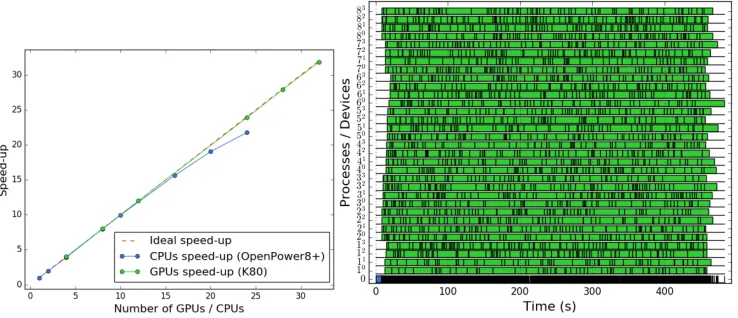
Figure 4.(Left) Speed-up of the application on a single IBM OpenPower8+node with 20 physical cores

(in blue) and speed-up on 8 nodes with 4 NVidia K80GPU’s each (in green); (Right) Work distribution in time of our dataset (2395 events), in this case, to the 32 availableGPU’s. The labelPd_{identifies aGPU,}

withPtheMPIprocess number anddtheGPUlocal identifier in the node. There is oneMPIprocess per node, except in the case of node 0 which is themasterMPIprocess. It takes in charge the I/O aspects

and the event distribution. One box in one timeline represents the computation of all the integrals of a same event.

is generally not the case withOpenCLprovided by NVidia. The portability has been tested on pre-exascale architectures: IBMOpenPOWERprocessor and NVidiaP100 GPU’s[11], espe-cially to validate the bridgeOpenCL/CUDA.

3.2 Performance

For this performance analysis, we used a production platform which offers an important

num-ber ofGPU’s for our application : the National Computing Center CC-IN2P3 at Lyon. Before moving to finer optimizations, it was important to understand the global behavior of the ap-plication and, to focus on two points first:

• How does the application scale in function of theGPUnumber? The application uses sev-eral asynchronous mechanisms, one at theMPIlevel (because the computing time varies a lot between two events), and the other at theOpenCLlevel which distributes the integral computation to the different devices attached to the node. Consequently, we want to make

sure that the concurent computations are not blocking each other.

• The acceleration ratio can be obtained. In other terms, what is the gain comparing the GPU’s MEM application with ourMPI/CPUversion? Can we enhance the performance of theGPU-MPI-MEMcode?

Each node of ourGPUplatform has 2 Intel Xeon E5-2640 processors, providing 2 x 8 physical cores rated at 2.6 GHz. In addition, each node is equipped with 4 KeplerGK-210 GPU’s on 2 NVidia K80 boards. The applications are compiled withgcc 5.3compiler with the-O 3optimization option and, for theGPU’s kernels, withnvcccompiler from theCUDA 8.0software environment.

Figure 4.(Left) Speed-up of the application on a single IBM OpenPower8+node with 20 physical cores

(in blue) and speed-up on 8 nodes with 4 NVidia K80GPU’s each (in green); (Right) Work distribution in time of our dataset (2395 events), in this case, to the 32 availableGPU’s. The labelPd_{identifies aGPU,}

withPtheMPIprocess number anddtheGPUlocal identifier in the node. There is oneMPIprocess per node, except in the case of node 0 which is themasterMPIprocess. It takes in charge the I/O aspects

and the event distribution. One box in one timeline represents the computation of all the integrals of a same event.

For all the performance analyses we add a time log at theMPIlevel to profile the moments when the event processing starts and finishes. The figure 4 (left) shows a excellent speed-up

(the ratio between the execution time of one code instanceieone MPI process, divided by the execution time of N instancesieN MPI processes) up to 8 nodes i.e. 32GPU’s. This can be explained by the very small time overhead of the communications and the event scheduling, compared to the average time to process an event. The figure 4 (right) shows that there is no delay between two event processing and that all the dataset is performed in impressive com-puting time: less than 500 seconds. Because the number of integrals per event to compute, as well as their kind (dimensionality) vary, the processing time for a single event fluctuates in a large range of values.

This remarkable gain is not only attributable to theGPU’s. A 3-4 factor is commonly conceded for the gain between an HPC node and aGPUdevice but also the kernel recoding in "flat" C avoiding the hidden overheads of the method calls in cascade ways. The other point is that theOpenCLorCUDAprogramming paradigm, based on data-parallel model, naturally vectorizes and is easily parallelized by the compilers.

4 Conclusion

The MEM is a powerful classification tool used for signal extraction in thettH analysis. It however requires a significant amount of computations. Its deployment onGPU’s platform has remarkably accelerated the computing time. We demonstrate in this paper that there is a high added value in using simultaneously a great number of GPU’s for ourttHanalysis: 55 days with one core, 14 hours with 96 cores and less than 500 seconds on 32GPU’s platform. Thanks to this computing time speed-up, the analyzers can now run the analysis multiple times. More checks can thus be carried out, and more analyses improvements be tested. This improvement however comes with a price: theOpenCLorCUDAprogramming paradigm forces to write the code or the kernels which are easy to parallelize/vectorize by the compiler,

explaining this important gain.

Nevertheless, it is a tedious and cumbersome task to transform C++code to C kernels.

In the future we will focus on this problem avoiding to penalize the extensibility of this implementation to other models. Using the MadGraph code-generation capability could be a way.

Today, theGPU-MPI-MEMversion is used to analyze the new data-taken at LHC. In the future with the High-Luminosity LHC upgrade, the computing power required will drastically increase, due to the larger data taking rate and the larger complexity of the events. Our GPU’s-based MEM analysis is ready to assimilate this data increase, thus freeing the LHC Computing Grid resources from such heavy computating analyses.

5 Acknowledgements

This work has been funded by the P2IO LabEx (ANR-10-LABX-0038) in the framework “Investissements d’Avenir” (ANR-11-IDEX-0003-01) managed by the French National Re-search Agency (ANR).

References

[1] Sirunyan A. M.et al.(CMS Collaboration),Observation of ttH Production, Phys. Rev.¯ Lett.120, 231801 (2018)

[2] Aad G.et al.(ATLAS Collaboration),Observation of a new particle in the search of the Standard Model Higgs boson with the ATLAS detector at the LHC, Phys. Lett. B716, 1 (2012)

[3] Chatrchyan S.et al.(CMS Collaboration),Observation of a new boson at a mass of 125 GeV with the CMS experiment at the LHC, Phys. Lett B71630 (2012)

[4] CMS Collaboration, Evidence for the Higgs boson decay to a bottom quark-antiquark pair, Phys. Lett. B780501 (2018)

[5] CMS Collaboration,Observation of the Higgs boson decay to a pair of tau leptons, Phys. Lett. B779283 (2017)

[6] CMS Collaboration, An event candidate for the production of a top quark and top anti-quark pair in conjunction with a Higgs Boson in the CMS detector, https://cds.cern.ch/record/2621446, (2018)

[7] Abazov V.M.et al.(DØ Collaboration),A precision measurement of the mass of the top quark, Nature429, 638–642 (2004)

[8] T. Strebler, thesisProbing the Higgs coupling to the top quark at the LHC in the CMS experiment, chap. 4 & 5 (2017)

[9] Schouten D., DeAbreu A. and Stelzer B.Accelerated Matrix Element Method with Par-allel Computing, Computer Physics Communications, Volume 192, pages 54-59 (2015) [10] Hagiwara K., Kanzaki J., Li Q., Okamura N. and Stelzer T.Fast computation of

Mad-Graph amplitudes on graphics processing unit (GPU), European Physical Journal732608 (2013)

[11] Hautreux G. et al., Pre-exascale Architectures: OpenPOWER Performance and Us-ability Assessment for French Scientific Community, ISC International Workshops 2017: 309-324 (2017)

[12] Lepage G. P., A New Algorithm for Adaptive Multidimensional Integration, J.Comput.Phys.27:192 (1978)

[13] Kanzaki J., Monte Carlo integration on GPU, European Physical Journal C,71:1559 (2011)

[14] Stone J E, Gohara D, and Shi G.Opencl: A parallel programming standard for hetero-geneous computing systems IEEE, Computing in Science&Engeneering,12(3), p. 66-73 (2010).

[15] Gropp W., Lusk E. and Skjellum A.,Using MPI: portable parallel programming with the message-passing interface, MIT Press Cambridge MA, USA (1994)

[16] Brun R. and Rademakers F., ROOT - An Object Oriented Data Analysis Framework, Nucl. Inst. & Meth. in Phys. Res. A,389:1-2 p. 81-86 (1997)

[17] Alwall J., Herquet M., Maltoni F., Mattelaer O. and Stelzer T.,MadGraph 5 : Going Beyond, JHEP 1106 128. arXiv:1106.0522, (2011)

[18] Grasseau G.et al.,Matrix element method for high performance computing platforms, CHEP 2015, J. Phys.: Conf. Ser. 664, p. 92009 (2015)

[19] Whalley M. R., Bourilkov D. and Group R. C., The Les Houches accord PDFs (LHAPDF) and Lhaglue, arXiv:hep-ph/0508110 (2005)