A Comparison Study on Criteria to Select the Most
Adequate Weighting Matrix
Marcos Herrera1,‡ , Jesus Mur2,‡ and Manuel Ruiz3, *
1 CONICET-IELDE, Universidad Nacional de Salta (Argentina); [email protected] 2 Universidad de Zaragoza (Spain); [email protected]
3 Universidad Politécnica de Cartagena (Spain); [email protected] * Correspondence:[email protected]; Tel.: +34-968325901
‡ These authors contributed equally to this work.
Version November 8, 2018 submitted to Preprints
Abstract:The practice of spatial econometrics revolves around a weighting matrix, which is often
1
supplied by the user on previous knowledge. This is the so calledWissue. Probably, the aprioristic
2
approach is not the best solution although, nowadays, there few alternatives for the user. Our
3
contribution focuses on the problem of selecting aWmatrix from among a finite set of matrices, all
4
of them considerer appropriate for the case. We develop a new and simple method based on the
5
Entropy corresponding to the distribution of probability estimated for the data. Other alternatives,
6
which are common in current applied work, are also reviewed. The paper includes a large Monte
7
Carlo to calibrate the effectiveness of our approach compared to the others. A well-known case study
8
is also included.
9
Keywords:Weights matrix, Model Selection, Entropy, Monte Carlo
10
1. Introduction 11
Let us begin with a mantra: the weighting matrix is the most characteristic element in a spatial
12
model. Most scholars agree with this popular commonplace. In fact, spatial models deal primarily with
13
phenomena such as spillovers, trans-boundary competition or cooperation, flows of trade, migration,
14
knowledge, etc. in complex networks. Rarely does the user know about how these events operate in
15
practice. Indeed, they are mostly unobservable phenomena which are, however, required to build the
16
model. Traditionally the gap has been solved by providing externally this information, in the form of a
17
weighting matrix. As an additional remark, we should note thatWis not the unique solution to deal
18
with such kind of unobservables (1, for example, develop a latent variables approach that does not
19
need ofW), but is the most simple.
20
Hayset al.[2] give a sensible explanation about the preference for a predefinedW. Network
21
analysts are more interested in the formation of networks, taking units attributes and behaviors as
22
given. This is spatial dependence due to selection, where relations of homophily and heterophily are
23
crucial. The spatial econometricians are more interested in what they call’computing the effects of alters 24
actions on ego’s actions through the network’; in this case, the patterns of connectivity are taken as given.
25
This form of spatial dependence is due to the influence between the individuals, and the notions of
26
contagion and interdependence are capital. So, if the network is predefined, why not supplying it
27
externally?
28
However, beyond this point, theWissue han been frequent cause of dispute. In the early stages,
29
terms like ’join’ or ’link’ were very common (for instance, in3, or4). The focus at that time was mainly
30
on testing for the presence of spatial effects, for which is not so important the specification of a highly
31
detailed weighting matrix; contiguity, nearness, rough measures of separation may be appropriate
32
notions for that purpose. The work of Ord [5] is a milestone in the evolution of this issue because of its
33
strong emphasis on the task of modelling spatial relationships. It is evident that the weights matrix
34
needs more attention if we want to avoid estimation biases and wrong inference. Anselin [67] puts
35
theWmatrix in the center of the debate about specification of spatial models, but, after decades of
36
practicing, the question still remains unclear.
37
The purpose of the so-calledWis to ’determine which ... units in the spatial system have an influence on 38
the particular unit under consideration ... expressed in notions of neighborhood and nearest neighbor’ relations,
39
in words of Anselin [6, p.16] or ’to define for any set of points or area objects the spatial relationships that 40
exist between them’ as stated by Haining [8, p. 74]. The problem is how should it be done.
41
Roughly speaking, we may distinguish two approaches: (i) specifying W exogenously; (ii)
42
estimatingW from data. The exogenous approach is by far the most popular and includes, for
43
example, use of a binary contiguity criterion, k-nearest neighbours, kernel functions based on distance,
44
etc. The second approach uses the topology of the space and the nature of the data, and takes many
45
forms.We find ad-hoc procedures in which a predefined objective guides the search such as the
46
maximization of Moran’sIin Kooijman [9] or the local statistical model of Getis and Aldstadt [10].
47
Benjanuvatra and Burridge [11] develop a quasi maximum-likelihood,QML, algorithm to estimate the
48
weights inWassuming partial knowledge about the form of the weights. More flexible approaches are
49
possible if we have panel information such as in Bhattacharjee and Jensen-Butler [12] or Beenstock and
50
Felsenstein [13]. Endogeneity of the weight matrix is another topic introduced recently in the field
51
(i.e.,14), which connects with the concept ofcoevolutionput forward by Snijderset al.[15] and based
52
on the assumption that, in the long run, network connectivity must evolve endogenously with the
53
model. Much of the recent literature on spatial econometrics revolves around endogeneity, but our
54
contribution pertains to the exogenous approach where remains most part of the applied research.
55
Before continue, we may wonder if theWissue, even in our context of pure exogeneity, is really
56
a problem to worry for or it is thebiggest mythof the discipline as claimed by LeSage and Pace [16].
57
Their argument is that only dramatic different choices forWwould lead to significant differences in
58
the estimates or in the inference. We partly agree with them in the sense that is a bit silly to argue
59
whether it is better the 5 or the 6 nearest-neighbor matrix; surely there will be almost no difference
60
between the two. However, there is consistent evidence, obtained mainly by Monte Carlo [17–20]
61
showing that the misspecification ofWhas a non-negligeable impact on the inference of the coefficients
62
of spatial dependence and other terms in the model. Moreover, the magnitude of the bias increases for
63
the estimates of the marginal direct/indirect effects. So, we are not pretty sure that ’far too much effort 64
has gone into fine-tunning spatial weight matrices’ as stated by LeSage and Pace [16]. Our impression is
65
that any useful result should be welcomed in this field and, especially, we need practical, clear guides
66
to approach the problem.
67
Another question of concern are the criticisms of Gibbons and Overman [21]. As said, it is
68
common in spatial econometrics to assume that the weighting matrix is known, which is the cause of
69
identification problems; this flaw extends to the instruments, moment conditions, etc. There is little
70
to say in relation to this point. In fact, spatial parameters (i.e.,ρ) and weighting matrix,W, are only 71
jointly identified (we do estimateρW). Hayset al.[2] and Bhattacharjee and Jensen-Butler [12] agree in 72
this point.
73
Bavaud [22, p. 153], given this controversial debate, was very skeptic, ’there is no such thing as 74
“true”, “universal” spatial weights, optimal in all situations’ and continues by stating that the weighting
75
matrix ’must reflect the properties of the particular phenomena, properties which are bound to differ from field 76
to field’. We share his skepticism; perhaps it would suffice with a ’reasonable’ weighting matrix, the
77
best among those considered. In practical terms, this means that the problem of selecting a weighting
78
matrix can be interpreted as a problem of model selection. In fact, different weighting matrices result
79
in different spatial lags of the variables included in the model and different equations with different
80
regressors amounts to a model selection problem.
81
As said, our intention is to offer new evidence to help the user to select the most appropriateW 82
matrix for the specification. Section 2 revises four selection criteria that fit well into the problem of
83
selecting a weighting matrix from among a finite set of them. Section 3 presents the main features of
the Monte Carlo solved in the fourth Section. Section 5 includes a well known case study which is
85
revised in the light of our findings. Sixth Section concludes.
86
2. Criteria to select a W matrix from among a finite set 87
TheWissue has been present in the literature on spatial econometrics since very early. However
88
the case of choosing one matrix from among a finite set of them is relatively recent. First, we review
89
the literature devoted to theJtest and then we moved to the selection criteria, Bayesian methods and a
90
new procedure based on Entropy.
91
Anselin [23] poses formally the problem suggesting aCox statistic derived in a framework
92
of non-nested models. Leenders [24], on this basis, elaborates a J-test using classical augmented
93
regressions. Later on, Kelejian [25] extends the approach ofLeendersto aSACmodel, with spatial
94
lags of the endogenous variable and in the error terms, usingGMMestimates. Piras and Lozano [26]
95
confirm the adequacy of theJ-test to compare different weighting matrices stressing that we should
96
make use of a full set of instrument to increaseGMMaccuracy. Burridge and Fingleton [27] show that
97
the Chi-square asymptotic approximations for theJ-tests produces irregular results, excessively liberal
98
or conservative in a series of leading cases; they suggest a bootstrap resampling approach. Burridge
99
[28] focuses on the propensity of the spatialGMMalgorithm to deliver spatial parameter estimates
100
lying outside the invertibility region which, in turn, affects the bootstrap; he suggest the use of aQML 101
algorithm to remove the problem. Kelejian and Piras [29] generalized and modify the original version
102
ofKelejianto account for all the available information, according to the findings ofPiras and Lozano.
103
Finally, Kelejian and Piras [30] adapt theJtest to a panel data setting with unobserved fixed effects
104
and additional endogenous variables which reinforces the adequacy of theGMMframework. Another
105
milestone in theJtest literature is Hagemann [31], who copes with the reversion problem originated
106
by the lack of a well defined null hypothesis in the test. He introduces the minimumJtest,MJ. His
107
approach is based on the idea that if there is a finite set of competing models, only the model with the
108
smallestJstatistic can be the correct one. In this case, theJstatistic will converge to the Chi-square
109
distribution but will diverge if none of the models is correct. The author proposes a wild bootstrap to
110
test if the model with the minimumJis correct. This approach has been applied by Debarsy and Ertur
111
[20] to a spatial setting with good results.
112
In the Monte Carlo that follows, we know that there is a correct model so are going to use only
113
the first part of the procedure ofHagemann. Assuming a collection ofmdifferent weighting matrices,
114
such as:W ={W1;W2; ...;Wm}, theMJapproach works as follows: 115
1. We need the estimates of themmodels; in each case, the same equation is employed but with a
116
different weighting matrix belonging toW. Following Burridge [28] and given that our interest
117
lies on the small sample case, the models are estimated byML.
118
2. For each model, we obtain the battery ofJstatistics as usual, after estimating, also byML, the
119
corresponding extended equations.
120
3. The chosen matrix is the one associated with the minimumJstatistic. We do not test if this matrix
121
is really the correct matrix.
122
Another popular method for choosing between models deals with the so-calledInformation Criteria.
123
Most are developed around a loss function, such as theKullback-Leibler,KL, quantity of information
124
which measures the closeness of two density functions. One of them corresponds to the true probability
125
distribution that generated the data, obviously not known, the other is the distribution estimated
126
from the data. The criteria differ in the role assigned to the aprioris and in the way of solving the
127
approximation to the unknown true density function [32]. The two most common procedures are the
128
AIC[33] and the BayesianBICcriteria [34]. The first compares the models on equal basis whereas the
129
second incorporates the notion of model of the null. Both criteria are characterized by their lack of
130
specificity in the sense that the selected model is the closest to the true model, as measured byKL. We
131
should note that, as indicated by Potscher [35], a good global fit does not mean that the model is the
best alternative to estimate the parameters of interest. AICandBIClead to single expressions that
133
depend on the accuracy of theMLestimation plus a penalty term related to the number of parameters
134
entering the model; that is:
135
AIC(k): −2l(γ) +e 2k, BIC(k): −2l(γ) +e klog(n),
)
(1)
wherel(γ)e means the estimated log-likelihood at theMLestimates,γe,kis the number of non-zero 136
parameters in the model and nthe number of observations. For the case that we are considering
137
the models only differ in the weighting matrix, sokandnare the same in every case. This means
138
that the decision depends on the estimated log-likelihood, or on the balance between the estimated
139
variance and the Jacobian term. Note that, for a standard spatial model of, i.e.,SLMtype we can write:
140
l(γ)e ∝log h
1
e
σn|I−ρeW| i
, beingσthe standard deviation andρthe corresponding spatial dependence 141
coefficient. To minimize any of the two statistics in (1) the objective is to maximize the concentrated
142
estimated log-likelihood,l(γ)e . The same as before, theInformation Criteriaapproach implies: 143
1. Estimate byMLof themmodels corresponding to each weighting matrix inW.
144
2. For each model, we obtain the corresponding AICstatistic (BICproduces the same results).
145
3. The matrix in the model with minimumAICstatistic should be chosen.
146
An important part of the recent literature on spatial econometrics has Bayesian basis; this extends
147
also to the topic of choosing a weighting matrix. The Bayesians are well equipped to cope with these
148
type of problems using the concept ofposterior probabilityas the basis for taking a decision. There are
149
excellent reviews in Hepple [363738], Besag and Higdon [39] and especially, LeSage and Pace [40]. For
150
the sake of completeness, let us highlight the main points in this approach.
151
The analysis is made conditional to a model, which is not under discussion. Moreover, we have a
152
collection ofmweighting matrices inW, a set ofkparameter inγ, some of which are of dispersion, 153
σ, others of position,β, and others of spatial dependence,ρ andθ, and a panel data set with nT 154
observations iny. The point of departure is the joint probability of data, parameters and matrices:
155
p(Wi;γ;y) =π(Wi)π(γ|Wi)L(y|γ;Wi), (2)
whereπ(·)are the prior distributions andL(y|γ;Wi)the likelihood foryconditional on the 156
parameters and the matrix. Bayes’ rule leads to the posterior joint probability for matrices and
157
parameters:
158
p(Wi;γ|y) = π(Wi)π(γ|Wi)L(y|γ;Wi)
L(y) , (3)
whose integration over the space of parameters,γ∈Υ, produces the posterior probability for 159
matrixWi: 160
p(Wi|y) = Z
Υ
p(Wi;γ|y)dγ. (4)
The presence of spatial structures in the model complicates the resolution of (4) which usually
161
requires of numerical integration. The priors are always a point of concern and, usually, practitioners
162
prefer diffuse priors. LeSage and Pace [40, Section 6.3] suggestπ(Wi) = m1 ∀i, aN IGconjugate prior 163
forβandσwhereπβ(β|σ)∼N
β0;σ2(κX0X)−1
, beingXthe matrix of the exogenous variables
164
in the model, andπ(σ)a inverse gamma, IG(a,b). For the parameter of spatial dependence they 165
suggest aBeta(d,d)distribution, beingdthe amplitude of the sampling space ofρ. The defaults in the 166
MATLAB codes of LeSage [41] areβ0=0,κ=10−12anda=b=0. In sum, theBayesianapproach 167
implies the following:
1. Fix the priors for all the terms appearing in the equation. In this point, we have followed the
169
suggestions ofLeSage and Pace.
170
2. For each matrix, obtain the corresponding posterior probability of (4) for which we need (i) solve
171
theMLestimation of the corresponding model and (ii) solve the numerical integration of (4).
172
3. The matrix chosen will be that associated with the highest posterior probability.
173
This paper advocates for a selection procedure based on the notion ofEntropy, which is used as
174
a measure of the information contained in a distribution of probability. Let us assume an univariate
175
continuous variable,y, whose probability density function isp(y); then,Entropyis defined as:
176
h(p) =− Z
Ip(y)logp(y)dy, (5)
beingIthe domain of the random variabley. As known, higherEntropymeans less information
177
or, what is the same, more uncertainty abouty. Our case fits with Shannon’s framework (42): we
178
observe a random variable,y, and there is a finite set of rival distribution functions capable of having
179
generated the data. Our decision problem is well defined because each distribution function differs
180
from the others only in the weighting matrix; the other elements are the same. However, we are not
181
interested in the Laplacian principle of indifference (select the density with maximumEntropy, less
182
informative, to avoid uncertain information). Quite the opposite: in our case there is no uncertain
183
information and we are looking for the more informative probability distribution so our objective is to
184
minimizeEntropy.
185
As with the other three cases, the application of this principle requires the complete specification
186
of the distribution function, which means that the user knows the form of the model (equations7 187
to9below, except theWmatrix); additionally we add a Gaussian distribution. Next, we should
188
remind that for the case of a(n×1)multivariate normal random variable,y∼N(µ;Σ), the entropy
189
is: h(y) = 12
n+log (2π)n|Σ|
. This measure does not depend, directly, on first order moments
190
(parameters of position of the model) but on second order moments (dependence and dispersion
191
parameters). For example, in the case of theSLMof (9) below, the entropy is:
192
h(y)SDM = 1
2
nT+log((2πσ2 nT
B
0B−1
)) (6)
whereB= (I−ρW). Note that the covariance matrix foryin theSDMisV(y) =B−1V(u)B0−1. 193
If uis indeed a white noise random term with variance σ2, the covariance matrix of y is simply 194
V(y) =σ2(B0B)−1. Let us note that the covariance matrix ofyin theSDMof (7) coincides with that 195
of theSLMcase. The covariance matrix for theSDEMequation isV(y) =σ2(B0B), everything else 196
remains the same.
197
In order to apply theEntropycriterion we must must go through the following steps:
198
1. Estimate each one of themversions of the model that we are considering. As said, each models
199
differs only in the weighting matrix. We obtain theMLestimates for reasons given above.
200
2. For each model, we obtain the corresponding value of theEntropy, in thehi;i=1, 2, ...,mstatistic. 201
3. The decision criterion consists in choosing the weighting matrix corresponding to the model
202
with minimum value of theEntropy.
203
3. Description of the Monte Carlo 204
This part of the paper is devoted to the design of the Monte Carlo conducted in the next Section
205
in order to to calibrate the performance of the four criteria presented so far for selectingW: theMJ 206
procedure, theBayesianapproach, theAICcriterion and theEntropymeasure. The objective of the
207
analysis is to identify and select the matrix that intervened in the generation of the data. Moreover, our
208
focus is on small sample sizes. As will be clear below, the four criteria have good behaviour even in
209
small samples, so it is not necessary to employ very large sample sizes
We are going to simulate a panel setting, with three of the most commonDGPsin the applied
211
literature on spatial econometrics; namely, the spatial Durbin Model,SDMof (7), the spatial Durbin
212
error model,SDEMin expression (8) and the spatial lag model of (9),SLM.1
213
yit =β0+ρ n
∑
j=1ωijyjt+xitβ1+θ n
∑
j=1ωijxjt+εit, (7)
yit =β0+xitβ1+θ n
∑
j=1ωijxjt+uit,uit =ρ n
∑
j=1ωijujt+εit. (8)
yit =β0+ρ n
∑
j=1ωijyjt+xitβ1+εit, (9)
Only one exogenous regressor,xvariable, appears in the right hand side of the equations whose
214
observations are obtained from a normal distribution,xit ∼i.i.d.N 0;σx2, whereσx2= 1; the same 215
applies with respect to the error terms:εit∼i.i.d.N 0;σε2, whereσε2=1. The two variables are not 216
related,E(xitεit) =0. Our space is made of hexagonal pieces which are arranged regularly, one next 217
to the others without discontinuities nor empty spaces.
218
One weighting matrix appears in the three equations, which plays a central role in the functioning
219
of the model. As said before, the weighting matrix is not observable and the user must take decisions
220
to resolve the uncertainty. The problem consists in choosing one matrix from among a finite set of
221
alternatives which in our simulation are composed by three candidates:W1is built using the traditional 222
contiguity criterion between spatial units; the weights inW2are the inverse of the distance between 223
the centroids of the spatial units,W2=
n
ωij= d1ij;i6=j o
; whereasW3incorporates a cut-off point to 224
the connections inW2, so thatW3=
n
ωij= d1ij;i6=j i f j∈ N4(i); 0otherwise
o
beingN4(i)the set of 225
4 nearest neighbors toi. To keep things simple, the same weighting matrix plays with the endogenous
226
and exogenous variables in (7) and with the exogenous and error terms in (8). Following usual practice,
227
every matrix has been row-standardized. Due to the row-standardization, the three matrices are non
228
nested in the sense that the sequence of weights are different among them.
229
Three different small cross-sectional sample sizes,n, have been used n ∈ {25, 49, 100}; that
230
is enough because higher values of this parameter only improves marginally the results. For the
231
same reason, the number of cross-sections in the panel,T, are limited to only three,T ∈ {1, 5, 10}.
232
The values for the coefficient of spatial dependence, ρ, ranges from negatives to positives, ρ = 233
{−0.8,−0.5,−0.2, 0.2, 0.5, 0.8}. Other global parameters are those associated with the constant term,
234
β0=1, thexvariable,β1∈ {1, 5}, and its spatial lag,θ∈ {1, 5}. 235
In sum, each case consists in:
236
• Generate the data using a given weighting matrix,Wk,k=1, 2, 3 and a spatial equation,SLM, 237
SDMorSDEM. There are 216 cases of interest for each equation (6 values inρ, 3 values inn, 3 238
values inT, 2 values inβ1and 2 values inθ). 239
• The spatial equation is assumed to be known so the model can be estimated by maximum
240
likelihood,ML, once the user supplies aWmatrix.
241
• Compute the four selection criteria, MJ,Posterior probability,Entropyand AIC for the three
242
alternative weighting matrices for each draw.
243
• Select the corresponding matrix according to each criterion and compare the result with thetrue 244
matrix in theDGP.
245
• The process has been replicated 1, 000 times.
246
Note that the selection of the matrix is made conditional on a correct specification of the equation.
247
We are perfectly aware that this dichotomy is artificial; in fact, both decisions are intimately related
248
because the same matrix, but in different equations, plays different roles and bears different information.
249
However, this point is not further developed in the present paper. In order to give some intuition,
250
we include the results corresponding to the case of a wrong specification (i.e, estimate aSDMmodel
251
whereas the true model in theDGPis aSDEM).
252
4. Results of the Monte Carlo 253
This Section summarizes the results obtained in the Monte Carlo. Let us advance an little spicy:
254
in strictly quantitative terms, theEntropymeasure is the best criterion. What is more surprising, the
255
Bayesianapproach is marginally better than the AIC, but only when the amount of information is
256
large and there is positive spatial correlation. Finally, theMJapproach is the worse alternative among
257
the four criteria. The last two observations are a bit surprising given the strong support that the two
258
procedures have received in the literature. Table1presents the percentage of correct selections attained
259
by each criterion after aggregating all the experiments in the Monte Carlo. A cell in bold indicates that
260
the respective criterion reaches the maximum rate of correct selections.
261
Table 1.Percentage of correct selections. Aggregated results
ρ h(y) Bayes MJ AIC
−0.8 83.8 83.2 50.7 84.4 −0.5 71.4 69.7 52.8 71.4 −0.2 55.9 49.4 54.2 54.6 0.2 60.8 54.6 58.3 60.5 0.5 75.7 73.6 58.2 73.5 0.8 85.9 85.4 53.6 78.7
AVERAGE 72.3 69.3 54.6 70.5
Entropydominates in 5 out of the 6 cases presented in the Table, and is the second in the sixth
262
case;AICleads in two cases, is second in two and third in another two cases.Bayesdoes not do very
263
well for small values of the spatial coefficient (is fourth in±0.2) and the curve of correct selections of
264
theMJis very flat.
Figure 1.Percentages of correct selections, disaggregated bynandT
CASE:n=25 CASE:T=1
CASE:n=49 CASE:T=5
CASE:n=100 CASE:T=10
Figure1disaggregates the accumulated percentages by number of spatial units, left, or number
266
of cross-sections, right. Note that in each case, the data represent aggregated percentages (i.e, in
267
the casen =25 we aggregate the three cross-sections corresponding toT = 1,T =5 andT = 10).
268
These courves ratifies the ordering set out above. Note the asymmetry in all the curves and the
269
strange behaviour of theMJcriterion that produces worst results at the extremes of the interval for
270
ρ. The other three criteria react positively to increases in the sample size (both innor inT). Overall, 271
the improvement is more relevant according toTthan ton, specially for high values of the spatial
272
coefficient.
273
Tables2to Table5present the details by type ofDGP. A quick look at the Tables reveals that bold
274
percentages are concentrated, mainly, in theEntropyandAICcolumns.
275
The prevalence of theEntropycriterion is quite regular (the exception is theSDEMprocess where
276
AIChas better results). The preference extends to the case of correctly specified models, as in Tables
2,3and4, and also for misspecified equations, as in Table5, for negative and especially for positive
278
values of the spatial coefficient, for small and large number of individuals in the sample (n) and for
279
simple to large panels (T). Overall,Entropyattains the highest rate in 48% of the 180 cases in Tables2 280
to5.
281
The complete relation of results for the 864 different experiments in the MC (3ns, 3Ts, 6ρs, 2βs, 282
2θs and four configurations for the DGP/estimated equation pair) appear in Tables10to21in the 283
Appendix. Let us note the good results attained in the case of small samples (n=25 andT=1) where
284
the average rate of correct selections forEntropyandAICis above 40% criteria (a little worse for the
285
other two). The percentage exceeds 60% at the extremes of the spatial parameter interval,±0.8. The
286
average rate improves upto 65% - 75%, for the case ofn =25 andT =5 and continues improving
287
whenT= 10, where most cases have a rate of correct selections above 90%. In general, the rate of
288
correct selections is nearly 100%, using 5 to 10 cross-sections.
289
Table 2.Average percentage of correct selections. DGP: SDM. Equation estimated: SDM.
Aggregated by cross-section, sample size (n) Aggregated by time series, sample size (T)
ρ h(y) Bayes MJ AIC ρ h(y) Bayes MJ AIC
n=25
−0.8 78.1 77.8 52.4 79.6
T=1
−0.8 67.4 66.2 39.4 68.8 −0.5 62.9 62.5 52.0 61.8 −0.5 54.4 54.3 38.5 57.5 −0.2 53.5 48.7 53.1 50.2 −0.2 41.1 38.4 40.0 41.7
0.2 61.5 59.8 65.0 61.2 0.2 43.2 35.8 48.4 40.8 0.5 74.7 56.5 50.8 72.1 0.5 56.5 50.8 55.2 54.3 0.8 84.3 81.7 74.5 75.5 0.8 69.7 68.1 63.4 63.8
n=49
−0.8 88.9 88.7 57.6 90.1
T=5
−0.8 91.9 93.0 62.3 93.5 −0.5 76.4 77.5 58.6 78.7 −0.5 79.4 80.2 63.7 79.5
−0.2 59.6 55.5 58.6 58.8 −0.2 63.3 57.3 62.4 60.1 0.2 71.0 67.9 73.1 70.0 0.2 79.1 76.6 78.1 76.1 0.5 84.1 81.7 81.6 82.0 0.5 92.3 92.5 87.1 89.8 0.8 93.3 93.8 88.1 87.4 0.8 98.4 98.3 88.2 89.9
n=100
−0.8 94.4 94.3 63.9 95.2
T=10
−0.8 97.3 97.4 69.2 97.9 −0.5 87.3 87.2 66.6 88.7 −0.5 88.8 88.7 72.1 87.9
−0.2 67.6 61.9 62.8 66.6 −0.2 72.3 66.5 68.2 69.8 0.2 80.5 76.4 79.4 77.1 0.2 86.6 87.7 86.4 87.4 0.5 91.9 90.5 85.6 89.7 0.5 97.0 97.5 92.9 95.4 0.8 97.3 96.3 89.5 92.4 0.8 99.8 99.8 94.6 95.8
Table 3.Average percentage of correct selections. DGP: SDEM. Equation estimated: SDEM.
Aggregated by cross-section, sample size (n) Aggregated by time series, sample size (T)
ρ h(y) Bayes MJ AIC ρ h(y) Bayes MJ AIC
n=25
−0.8 80.5 77.3 56.7 82.5
T=1
−0.8 66.7 65.3 42.5 70.4 −0.5 69.6 65.2 57.5 69.6 −0.5 55.4 55.6 44.0 62.1 −0.2 59.6 52.5 56.5 58.2 −0.2 42.5 42.8 43.8 49.3
0.2 55.6 52.4 56.9 57.7 0.2 39.5 36.1 45.7 43.4 0.5 63.5 62.6 55.7 63.7 0.5 49.5 45.4 46.5 48.7 0.8 74.4 73.8 54.0 67.0 0.8 59.3 58.1 48.9 53.2
n=49
−0.8 88.1 88.5 64.5 91.0
T=5
−0.8 94.0 94.7 71.1 95.4 −0.5 78.2 78.8 65.6 81.9 −0.5 84.1 84.8 72.5 84.9 −0.2 64.6 62.6 65.2 66.3 −0.2 70.2 67.1 71.6 69.6 0.2 64.8 61.4 65.2 65.9 0.2 71.2 69.3 70.3 73.1
0.5 78.0 75.7 64.5 75.1 0.5 83.1 85.5 67.8 83.7 0.8 88.0 87.1 64.0 79.6 0.8 94.7 95.4 64.6 86.8
n=100
−0.8 95.1 95.8 75.1 96.4
T=10
−0.8 97.7 98.2 78.9 98.6 −0.5 88.9 91.3 76.4 92.1 −0.5 92.4 91.6 79.3 91.7
−0.2 74.2 75.1 76.4 77.2 −0.2 81.5 77.4 78.8 78.3 0.2 75.6 74.9 75.1 78.3 0.2 81.4 80.3 77.3 81.7
Table 4.Average percentage of correct selections. DGP: SLM. Equation estimated: SLM.
Aggregated by cross-section, sample size (n) Aggregated by time series, sample size (T)
ρ h(y) Bayes MJ AIC ρ h(y) Bayes MJ AIC
n=25
−0.8 58.7 59.7 27.3 58.3
T=1
−0.8 54.0 53.1 23.7 54.5 −0.5 41.9 36.2 27.0 38.4 −0.5 36.3 33.3 24.3 37.7 −0.2 28.3 15.8 28.3 26.5 −0.2 22.6 14.2 28.3 22.5 0.2 33.4 21.0 30.2 33.5 0.2 30.8 12.6 32.5 30.0 0.5 54.0 49.6 31.8 54.2 0.5 46.3 37.4 34.6 45.4 0.8 72.4 70.8 31.9 70.0 0.8 61.0 61.0 36.2 56.6
n=49
−0.8 73.6 73.2 22.1 74.4
T=5
−0.8 79.7 81.4 19.9 80.7
−0.5 53.2 47.7 25.4 51.5 −0.5 57.9 53.0 24.1 55.9
−0.2 32.3 17.9 28.9 30.5 −0.2 32.8 15.1 28.1 30.2 0.2 41.7 24.9 31.5 39.9 0.2 44.4 27.4 29.2 43.0 0.5 68.8 64.3 26.9 67.7 0.5 73.0 72.8 24.4 71.5 0.8 86.8 87.1 26.2 82.1 0.8 93.5 93.3 24.8 88.3
n=100
−0.8 86.7 87.0 12.0 87.6
T=10
−0.8 85.4 85.3 17.7 85.1
−0.5 68.0 65.2 18.0 68.3 −0.5 68.8 62.8 22.0 64.7
−0.2 37.8 22.2 27.1 36.3 −0.2 43.0 26.6 28.0 40.6 0.2 51.3 35.4 27.6 50.6 0.2 51.1 41.3 27.6 51.1
0.5 81.4 79.8 20.6 79.0 0.5 84.9 83.4 20.2 84.0 0.8 92.3 92.9 20.2 86.9 0.8 97.0 96.5 17.3 94.0
Table 5.Average percentage of correct selections. DGP: SDEM. Equation estimated: SDM.
Aggregated by cross-section, sample size (n) Aggregated by time series, sample size (T)
ρ h(y) Bayes MJ AIC ρ h(y) Bayes MJ AIC
n=25
−0.8 79.2 77.2 51.4 77.6
T=1
−0.8 66.2 66.0 38.1 68.9 −0.5 66.5 64.1 55.1 62.3 −0.5 54.3 55.5 40.8 58.1 −0.2 57.9 52.4 57.4 52.7 −0.2 42.2 40.2 42.3 42.7
0.2 54.8 54.0 59.1 55.4 0.2 38.2 32.3 44.8 37.7 0.5 62.8 62.4 55.9 59.4 0.5 46.4 42.3 45.4 43.6 0.8 71.9 72.2 42.5 59.4 0.8 55.1 54.1 42.5 47.3
n=49
−0.8 87.9 88.6 60.4 89.9
T=5
−0.8 92.3 92.3 64.3 91.7
−0.5 77.5 78.9 62.7 79.8 −0.5 83.3 81.6 67.4 80.0
−0.2 64.2 61.3 64.7 63.1 −0.2 69.4 63.4 69.5 64.5 0.2 64.8 60.7 65.5 64.1 0.2 71.9 68.5 69.4 70.9 0.5 75.1 73.5 63.2 70.2 0.5 82.2 83.9 65.7 78.2 0.8 84.3 84.3 47.1 72.1 0.8 92.2 93.7 44.3 77.9
n=100
−0.8 94.9 95.0 67.0 95.8
T=10
−0.8 97.2 97.2 72.6 96.9
−0.5 87.9 88.6 70.4 89.8 −0.5 89.9 89.9 76.1 88.8
−0.2 72.4 68.9 71.5 71.3 −0.2 78.6 74.9 77.7 75.6 0.2 74.9 70.0 71.1 73.4 0.2 80.8 80.2 77.0 80.5 0.5 85.9 85.9 68.2 83.3 0.5 91.8 92.5 72.0 87.9 0.8 92.7 93.3 39.6 84.4 0.8 98.3 98.8 38.3 87.6
In a similar vein, the increase in the cross-sectional size,n, maintaining constant the number of
290
cross-sections,T, also has positive effects in the four criteria. The rate of correct selections for the case
291
of a hundred of spatial units is above 70%, on average, for the case of a single cross-section (T=1),
292
but these percentages improve quickly if the time dimension of the panel increases.
293
The value of parameterβ1, as expected, has a weak impact in the four criteria; on the contrary, 294
the signal ofθ1plays a crucial role in theSDEMcase. Another interesting feature is the asymmetry of 295
the selection curves, that tends to be diluted withT. Negative spatial dependence helps to detect the
296
correctly weighting matrix, especially when the number of time cross-sections is small. The asymmetry
297
exists in Entropy, Bayes and AIC. However, the behavior of the MJ worsens in case of negative values
298
in parameterρ. 299
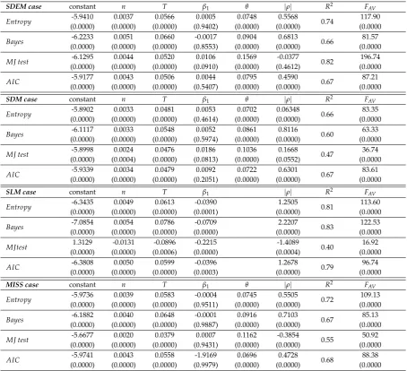
To complete the picture, we estimate a response-surface for each DGP/Estimated-equation
300
combination, with the aim of modelling the empirical probability of choosing the correct weighting
matrix for each criterion,pi. As usual, a logit transformation of the empirical probabilities is carried 302
out, so the estimated equation is:
303
log pi+ (2r) −1
1−pi+ (2r)−1 !
=p∗i =η+ziϕ+ei, (10)
wherepi∗is the logit transformation, often known as thelogit,rthe number of replications of each
304
experiment (1000 in all the cases);(2r)−1assures that thelogitis defined even when the probability
305
of correct selection is 0 or 1 (43);ηis an intercept term,zithe design matrix whose columns reflect 306
the conditions of each experiment,ϕis a vector of parameters andeithe error term assumed to be 307
independent and identically distributed (this assumption is reasonable if all experiments come from
308
the same study, as ours, and are obtained under identical circumstances;44). Let us remind that the
309
number of observations for eachresponse-surfaceequation is 216 (soi=1, 2, ..., 216). Table6shows the
310
results for the fourDGP/Estimated-equation combinations.
311
In general, the estimates confirm previous facts. The main factor influencing the empirical
312
probability of choosing the correct weights matrix is the spatial parameter, absolute value ofρin Table 313
6. Its contribution is crucial in the case of theBayesiancriteria and, to a lesser extend, also in the cases
314
ofEntroyand AIC. This parameter is not significant, for the case of the MJ approach andSDEM 315
processes whereas its contribution is negative in theSLMand in misspecified equations. The second
316
more influential factor is the parameterθ, associated to spatial spillovers. Its impact is beneficial for 317
all the cases though it appears to be more important for theMJ; the other three criteria are a bit less
318
sensitive. Sample size is also relevant in all the cases andT has a relatively higher impact thann.
319
Finally, as said before, parameterβ1is not significant in any circumstance, with the exception of the 320
SLMcase; this means that thesignal-to-noiseratio should not be a major factor to consider when the
321
problem is select the best weighting matrix.
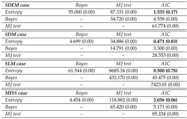
322
Table7completes theresponse-surfaceanalysis with theFtests of equality in the coefficients of
323
the estimates of Table6. According to the sequence ofF tests, the most dissimilar method is the
324
MJapproach, and thenBayes. On the other hand,EntropyandAICemerge as similar strategies to
325
compare weighting matrices; in fact, in what respect this simpleresponse-surfaceanalysis, they are
326
almost indistinguishable in the four types ofDGPs.
Table 6.Estimated response surfaces.
SDEM case constant n T β1 θ |ρ| R2 FAV
Entropy -5.9410 0.0037 0.0566 0.0005 0.0748 0.5568 0.74 117.90
(0.0000) (0.0000) (0.0000) (0.9402) (0.0000) (0.0000) (0.0000
Bayes -6.2233 0.0051 0.0660 -0.0017 0.0904 0.6813 0.66 81.57
(0.0000) (0.0000) (0.0000) (0.8553) (0.0000) (0.0000) (0.0000
MJ test -6.1295 0.0044 0.0520 0.0106 0.1569 -0.0377 0.82 196.74
(0.0000) (0.0000) (0.0000) (0.0910) (0.0000) (0.4612) (0.0000
AIC -5.9177 0.0043 0.0506 0.0044 0.0795 0.4590 0.67 87.21 (0.0000) (0.0000) (0.0000) (0.5407) (0.0000) (0.0000) (0.0000
SDM case constant n T β1 θ |ρ| R2 FAV
Entropy -5.8902 0.0033 0.0481 0.0053 0.0702 0.06348 0.66 83.35
(0.0000) (0.0000) (0.0000) (0.4614) (0.0000) (0.0000) (0.0000
Bayes -6.1117 0.0033 0.0548 0.0052 0.0861 0.8116 0.60 63.33
(0.0000) (0.0000) (0.0000) (0.5974) (0.0000) (0.0000) (0.0000
MJ test -5.8998 0.0024 0.0476 0.0186 0.1036 0.1668 0.47 36.74
(0.0000) (0.0004) (0.0000) (0.0813) (0.0000) (0.0552) (0.0000
AIC -5.9339 0.0034 0.0479 0.0092 0.0722 0.6301 0.67 83.61 (0.0000) (0.0000) (0.0000) (0.2051) (0.0000) (0.0000) (0.0000
SLM case constant n T β1 |ρ| R2 FAV
Entropy -6.3435 0.0049 0.0613 -0.0390 1.2505 0.81 113.60
(0.0000) (0.0000) (0.0000) (0.0001) (0.0000) (0.0000
Bayes -7.0854 0.0054 0.0786 -0.0709 2.2207 0.83 122.53
(0.0000) (0.0000) (0.0000) (0.0000) (0.0000) (0.0000
MJtest 1.3129 -0.0131 -0.0896 -0.2215 -1.4089 0.40 16.92
(0.0000) (0.0000) (0.0006) (0.0000) (0.0004) (0.0000
AIC -6.3808 0.0050 0.0599 -0.0396 1.2678 0.79 96.74
(0.0000) (0.0000) (0.0000) (0.0003) (0.0000) (0.0000
MISS case constant n T β1 θ |ρ| R2 FAV
Entropy -5.9736 0.0039 0.0583 -0.0004 0.0745 0.5505 0.72 109.13
(0.0000) (0.0000) (0.0000) (0.9511) (0.0000) (0.0000) (0.0000
Bayes -6.1882 0.0040 0.0648 -0.0001 0.0916 0.7103 0.67 85.13
(0.0000) (0.0000) (0.0000) (0.9887) (0.0000) (0.0000) (0.0000
MJ test -5.6677 0.0020 0.0379 0.0007 0.1162 -0.3854 0.55 50.92
(0.0000) (0.0000) (0.0000) (0.9431) (0.0000) (0.0000) (0.0000
Table 7.F test for the equality of coefficients in the response-surface estimates
SDEM case Bayes MJ test AIC Entropy 55.000 (0.00) 87.331 (0.00) 1.535 (0.17)
Bayes – 34.720 (0.00) 4.558 (0.00)
MJ test – – 61.774 (0.00)
SDM case Bayes MJ test AIC Entropy 4.699 (0.00) 34.886 (0.00) 0.471 (0.83)
Bayes – 14.791 (0.00) 3.300 (0.00)
MJ test – – 28.553 (0.00)
SLM case Bayes MJ test AIC Entropy 61.544 (0.00) 8685.34 (0.00) 0.500 (0.78)
Bayes – 432.170 (0.00) 45.475 (0.00)
MJ test – – 7423.01 (0.00)
MISS case Bayes MJ test AIC Entropy 4.454 (0.00) 118.882 (0.00) 2.056 (0.06)
Bayes – 65.420 (0.00) 5.171 (0.00)
MJ test – – 85.234 (0.00)
Note:p-value appear between brackets.
5. Empirical application 328
The case studied in this section is based on a well-known economic model. It is a model of
329
economic growth estimated by Ertur and Koch (2007) using a cross-section of 91 countries for the
330
period 1960–1995. The purpose of this section is to illustrate the use of the selection procedures
331
discussed before.
332
5.1. Study case: Ertur and Koch (2007) 333
Ertur and Koch [45] build a growth equation to model technological interdependence between
334
countries using spatial externalities. The main hypotheses of interaction is that the stock of knowledge
335
in one country produces externalities that cross national borders and spill over into neighboring
336
countries, with an intensity which decreases with distance. The authors use a geographical distance
337
measure.
338
The benchmark model assumes an aggregated Cobb-Douglas production function with constant
339
returns to scale in labour and physical capital:
340
Yi(t) =Ai(t)Kiα(t)L1i−α(t), (11)
whereYi(t)is output,Ki(t)is the level of reproducible physical capital,Li(t)is the level of labour, 341
andAi(t)is the aggregate level of technology specified as: 342
Ai(t) =Ω(t)kφi(t) n
∏
j6=iAδωi ij(t). (12)
The aggregate level of technologyAi(t)in a countryidepends on three elements. First, a certain 343
proportion of technological progress is exogenous and identical in all countries:Ω(t) =Ω(0)eµt, where 344
µis a constant rate of technological growth. Second, each country’s aggregate level of technology 345
increases with the aggregate level of physical capital per workerkφi(t) = (Ki(t)/Li(t))φwith parameter 346
φ∈[0; 1]capturing the strength of home externalities by physical capital accumulation. Finally, the 347
third term captures the external effects of knowledge embodied in capital located in a different country,
348
whose impact crosses national borders at a diminishing intensity,δ∈[0; 1]. The termsωijrepresent 349
the connectivity between countryiand its neighbours; these weights are assumed to be exogenous,
350
non-negative and finite.
351
Following Solow, the authors assume that a constant fraction of outputsi, in every countryi, is 352
annual rate of depreciation of physical capital for all countries, denotedτ. The evolution of output 354
per worker in countryiis governed by the usual fundamental dynamics of the Solow equation which,
355
after some manipulations, lead to a steady-state real income per worker [45, p. 1038, eq. 9]:
356
y=Ω+ (α+φ)k−αδWk+δWy. (13)
This is a spatially augmented Solow model and coincides with the predictor obtained by Solow
357
adding spillover effects. In terms of spatial econometrics, we have aSpatial Durbin Model,SDM, which
358
can be expressed as:
359
y=xβ+ρWy+Wxθ+ε. (14)
Equation (14) is estimated using information on real income, investment and population growth
360
for a sample of 91 countries for the period 1960−1995. Regarding the spatial weighting matrix,Ertur 361
and Kochconsider two geographical distance functions: the inverse of squared distance (which is
362
the main hypothesis) and the negative exponential of squared distance (to check robustness in the
363
specification). We also consider a third matrix based on the inverse of the distance.
364
Let us call the three weighting matrices asW1,W2andW3which are row-standardized:ωhij= 365
ωhij∗ / n ∑ j=1
ωhij∗ ; h=1, 2, 3 where: 366
ω∗1ij= (
0 i f i=j
d−ij2 otherwise ; ω
∗
2ij = (
0 i f i=j
e−2dij otherwise ; ω ∗
3ij= (
0 i f i=j
dij−1 otherwise , (15)
withdijas the great-distance between the capitals of countriesiandj. 367
The authors analyze several specifications checking for different theoretical restrictions and
368
alternative spatial equations. We concentrate our revision in the so-called non-restricted equation, in
369
the sense that it includes more coefficients than advised by theory. Table8presents the SDM version of
370
this equation using the three alternative weighting matrices specified before (the first two columns
371
coincide with those in Table I, columns 3-4, pp. 1047, of45). The last four rows in the Table show the
372
value of the selection criteria corresponding to each case.
373
The preferred model byErtur and Kochis the SDM/W1which coincides with the selection 374
attained by minimumEntropy,theBayesianposterior probability andAIC. The selection of theMJ 375
approach isW2. 376
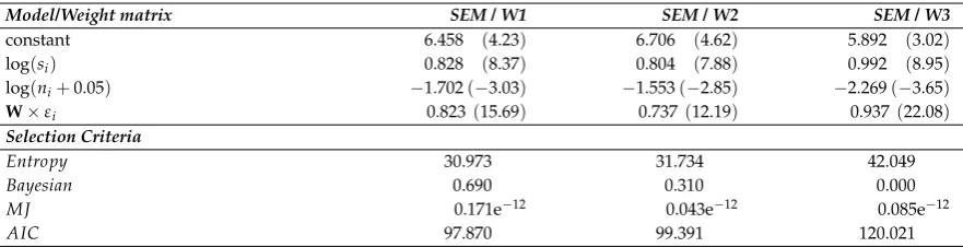
Other results inErtur and Koch refer to the Spatial Error Model version of the steady-state
377
equation of (13), orSEMmodel. The intention of the authors is to visualize the presence of spatial
378
correlation in the traditional non spatial Solow equations; we use this case as an example of selection of
379
weighting matrices in misspecified models. The main results appear in Table9(which can be compared
380
with columns 2-3 of Table II, in45, p. 1048).
Table 8.Ertur & Koch case. Unrestricted SDM estimates
Model/Weight matrix SDM / W1 SDM / W2 SDM / W3 constant 0.967−(0.51) 0.499−(0.27) 5.197−(0.99) log(s) 0.825−(8.26) 0.792−(7.62) 0.910−(8.49) log(n+0.05) −1.498(−2.64) −1.451(−2.62) −1.710(−2.67)
W×log(s) −0.326(−1.78) −0.378(−2.29) 0.500−(1.25)
W×log(n+0.05) 0.574−(0.68) 0.141−(0.18) 2.150−(1.01)
W×log(y) 0.742(10.70) 0.661−(9.01) 0.883(11.60) Selection Criteria
Entropy 28.001∗∗∗ 29.615∗∗∗ 34.615∗∗∗
Bayesian 0.864∗∗∗ 0.133∗∗∗ 0.003∗∗∗
MJ 11.158∗∗∗ 9.388∗∗∗ 10.208∗∗∗
AIC 95.885∗∗∗ 99.100∗∗∗ 109.132∗∗∗
Note:t-ratios appear between brackets.
Table 9.Ertur & Koch case. Unrestricted SEM estimates
Model/Weight matrix SEM / W1 SEM / W2 SEM / W3 constant 6.458−(4.23) 6.706−(4.62) 5.892−(3.02) log(si) 0.828−(8.37) 0.804−(7.88) 0.992−(8.95)
log(ni+0.05) −1.702(−3.03) −1.553(−2.85) −2.269(−3.65) W×εi 0.823(15.69) 0.737(12.19) 0.937(22.08)
Selection Criteria
Entropy 30.973 31.734 42.049
Bayesian 0.690 0.310 0.000
MJ 0.171e−12 0.043e−12 0.085e−12
AIC 97.870 99.391 120.021
Note:t-ratios appear between brackets.
The selection of the most adequateWmatrix does not change. Using the values ofEntropycriterion
382
we select the model in which intervenes the matrixW1, the same as with the Bayesian approach and 383
theAICcriterion;MJcontinues selectingW2. 384
6. Conclusion 385
Much of the applied spatial econometrics literature seems to prefer an exogenous approximation
386
to theWmatrix. Implicitly, it is assumed that the user has relevant knowledge with respect to the way
387
individuals in the sample interact. In recent years, new literature advocates for a more data driven
388
approach to theWissue. We strongly support this tendency, which should be dominant in the future;
389
however, our focus in this paper is on the exogenous approach.
390
The problem posed in the paper is very frequent in applied work: the user has a finite collection
391
of weighting matrices, they all are coherent with the case of study, and one needs to select one of them.
392
Which is the bestW? We can address this question using different proposals: theBayesianposterior
393
probability, theJapproach with all its variants, by means of simple model selection criteria, such as
394
AICorBICand several other alternatives not used in this study. We add a fourth one, based on the
395
Entropyof the estimated distribution function. This new criterionh(y)is a measure of uncertainty, and
396
fits well with theWdecision problem. Theh(y)statistics depends on the estimated covariance matrix
397
of the corresponding model offering a more complete picture of the suitability of the distribution
398
function (related to a particular choice ofW), to deal with the data at hand.
399
The conclusions of our Monte Carlo are very illuminating. First, we can confirm that it is possible
400
to identify, with confidence, the true weighting matrix (if it exists); in this sense, the selection criteria
401
do a good job. However, the four criteria should not be taken as indifferent, especially in samples of
402
small size (norT). The ordering is clear:Entropyin first place,AICandBayesian posterior probability
slightly worse, and thenMJ in the fourth position. As shown in the paper, the value of the spatial
404
parameter has a great impact to guarantee a correct selection, but this aspect is unobservable to the
405
researcher. However, the user effectively controls the amount of information involved in the exercise,
406
and this is also a key factor. The advice is clear: use as much information as you have because the
407
quality of the decision improves with the amount of information. Once again, the way the information
408
accrues is not neutral: the length of the time series in the panel is more relevant than the number of
409
cross-sectional units in the sample.
410
Our final recommendation for applied researchers is to care for the adequacy of the weighting
411
matrix and, in case of having various candidates, take a decision using well-defined criteria such as
412
theEntropy. The empirical application presented in Section 5 illustrates the procedure.
Author Contributions: conceptualization; methodology; formal analysis; writing original draft, review and 414
editing: Marcos Herrra, Jesus Mur and Manuel Ruiz 415
Funding:This research was funded by the Spanish Ministry of Economics grants numbers ECO2015-65758-P 416
and ECO2015-65637-P and Government of Aragon grant number S37_17R. This study is part of the collaborative 417
activities carried out under the program Groups of Excellence of the Region of Murcia, the Fundación Séneca, 418
Science and Technology Agency of the Region of Murcia Project 19884/GERM/15. 419
Conflicts of Interest:The authors declare no conflict of interest. 420
7. References 421
422
1. Oud, J.H.; Folmer, H. A structural equation approach to models with spatial dependence. Geographical
423
Analysis2008,40, 152–166. 424
2. Hays, J.C.; Kachi, A.; Franzese, R.J. A spatial model incorporating dynamic, endogenous network 425
interdependence: A political science application. Statistical Methodology2010,7, 406–428. 426
3. Moran, P.A. The interpretation of statistical maps. Journal of the Royal Statistical Society. Series B
427
(Methodological)1948,10, 243–251. 428
4. Whittle, P. On Stationary Processes in the Plane. Biometrika1954,41, 434–449. 429
5. Ord, K. Estimation methods for models of spatial interaction. Journal of the American Statistical Association
430
1975,70, 120–126. 431
6. Anselin, L.Spatial econometrics: Methods and models; Vol. 4, Kluwer Academic Publishers, Dordrecht, 1988. 432
7. Anselin, L. Under the hood issues in the specification and interpretation of spatial regression models. 433
Agricultural economics2002,27, 247–267. 434
8. Haining, R.P.Spatial data analysis: theory and practice; Cambridge University Press, 2003. 435
9. Kooijman, S. Some remarks on the statistical analysis of grids especially with respect to ecology. Annals of
436
Systems Research1976,5, 113–132. 437
10. Getis, A.; Aldstadt, J. Constructing the Spatial Weights Matrix Using a Local Statistic.Geographical Analysis
438
2004,36, 90–104. 439
11. Benjanuvatra, S.; Burridge, P. Qml estimation of the spatial weight matrix in the mr-sar model. Working
440
Paper 15/24. Department of Economics and Related Studies, University of York2015. 441
12. Bhattacharjee, A.; Jensen-Butler, C. Estimation of the spatial weights matrix under structural constraints. 442
Regional Science and Urban Economics2013,43, 617–634. 443
13. Beenstock, M.; Felsenstein, D. Nonparametric estimation of the spatial connectivity matrix using spatial 444
panel data.Geographical Analysis2012,44, 386–397. 445
14. Qu, X.; f. Lee, L. Estimating a spatial autoregressive model with an endogenous spatial weight matrix. 446
Journal of Econometrics2015,184, 209–232. 447
15. Snijders, T.A.; Steglich, C.E.; Schweinberger, M., Longitudinal models in the Behavioural ond Related 448
Sciences; Lawrence Erlbaum, 2007; chapter Modeling the co-evolution of networks and behavior, pp. 41–71. 449
16. LeSage, J.P.; Pace, R.K. The biggest myth in spatial econometrics.Econometrics2014,2, 217–249. 450
17. Florax, R.J.; Rey, S. The impacts of misspecified spatial interaction in linear regression models. InNew
451
directions in spatial econometrics; Anselin, L.; Florax, R., Eds.; Springer, 1995; pp. 111–135. 452
18. Franzese Jr, R.J.; Hays, J.C. Spatial econometric models of cross-sectional interdependence in political 453
science panel and time-series-cross-section data. Political Analysis2007,15, 140–164. 454
19. Lee, L.f.; Yu, J. QML estimation of spatial dynamic panel data models with time varying spatial weights 455
matrices.Spatial Economic Analysis2012,7, 31–74. 456
20. Debarsy, N.; Ertur, C. Interaction matrix selection in spatial econometrics with an application to growth 457
theory.Document de Recherche du Laboratoire d’Economie d’Orleans2016. 458
21. Gibbons, S.; Overman, H.G. Mostly pointless spatial econometrics? Journal of Regional Science2012, 459
52, 172–191. 460
22. Bavaud, F. Models for spatial weights: a systematic look.Geographical analysis1998,30, 153–171. 461
23. Anselin, L. Specification Tests on the Structure of Interaction in Spatial Econometric Models. Papers of the
462
24. Leenders, R. Modeling social influence through network autocorrelation: constructing the weight matrix. 464
Social Networks2002,24, 21–47. 465
25. Kelejian, H.H. A spatial J-test for model specification against a single or a set of non-nested alternatives. 466
Letters in Spatial and Resource Sciences2008,1, 3–11. 467
26. Piras, G.; Lozano, N. Spatial J-test: some Monte Carlo evidence. Statistics and Computing2012,22, 169–183. 468
27. Burridge, P.; Fingleton, B. Bootstrap inference in spatial econometrics: the J-test. Spatial Economic Analysis
469
2010,5, 93–119. 470
28. Burridge, P. Improving the J test in the SARAR model by likelihood-based estimation. Spatial Economic
471
Analysis2012,7, 75–107. 472
29. Kelejian, H.H.; Piras, G. An extension of Kelejian’s J-test for non-nested spatial models. Regional Science
473
and Urban Economics2011,41, 281–292. 474
30. Kelejian, H.H.; Piras, G. An Extension of the J-Test to a Spatial Panel Data Framework. Journal of Applied
475
Econometrics2016,31, 387–402. 476
31. Hagemann, A. A simple test for regression specification with non-nested alternatives.Journal of Econometrics
477
2012,166, 247–254. 478
32. Hansen, B.E. Challenges for econometric model selection.Econometric Theory2005,21, 60–68. 479
33. Akaike, H., 2nd International Symposium on Information Theory; Akademiai Kiodo, 1973; chapter 480
Information Theory and an Extension of the Maximum Likelihood Principle, pp. 267–281. 481
34. Schwarz, G. Estimating the dimension of a model.The annals of statistics1978,6, 461–464. 482
35. Potscher, B. Effects of model selection on inference. Econometric Theory1991,7, 163–185. 483
36. Hepple, L.W. Bayesian techniques in spatial and network econometrics: 1. Model comparison and posterior 484
odds. Environment and Planning A1995,27, 447–469. 485
37. Hepple, L.W. Bayesian techniques in spatial and network econometrics: 2. Computational methods and 486
algorithms. Environment and Planning A1995,27, 615–644. 487
38. Hepple, L.W. Bayesian model choice in spatial econometrics. InAdvances in Econometrics: Spatial and
488
Spatiotemporal Econometrics; LeSage, J.; Pace, K., Eds.; Emerald Group Publishing Limited, 2004; Vol. 18, pp. 489
101–126. 490
39. Besag, J.; Higdon, D. Bayesian analysis of agricultural field experiments. Journal of the Royal Statistical
491
Society: Series B (Statistical Methodology)1999,61, 691–746. 492
40. LeSage, J.; Pace, R.Introduction to spatial econometrics; Statistics: A Series of Textbooks and Monographs, 493
Chapman and Hall, CRC press, 2009. 494
41. LeSage, J. Spatial econometrics toolbox. available at: www. spatial-econometrics. com2007. 495
42. Shannon, C.; Weaver, C.The Mathematical Theory of Communication; University of Illinois Press: Urbana, 496
1949. 497
43. Maddala, G. Qualitative and limited dependent variable models in econometrics; Cambridge: Cambridge 498
University Press, 1983. 499
44. Florax, R.J.; De Graaff, T. The performance of diagnostic tests for spatial dependence in linear regression 500
models: a meta-analysis of simulation studies. InAdvances in spatial econometrics; Anselin, L.; Florax, R.; 501
Rey, S., Eds.; Springer, 2004; pp. 29–65. 502
45. Ertur, C.; Koch, W. Growth, technological interdependence and spatial externalities: theory and evidence. 503
Journal of applied econometrics2007,22, 1033–1062. 504
46. Munnell, A.H.; Cook, L.M.; others. How does public infrastructure affect regional economic performance? 505
New England economic review1990, pp. 11–33. 506
47. Millo, G.; Piras, G.; others. splm: Spatial panel data models in R.Journal of Statistical Software2012,47, 1–38. 507
48. Alvarez, I.C.; Barbero, J.; Zofio, J.L. A Panel Data Toolbox for MATLAB.Journal of Statistical Software2017, 508
76, 1–27. 509
19
of
30
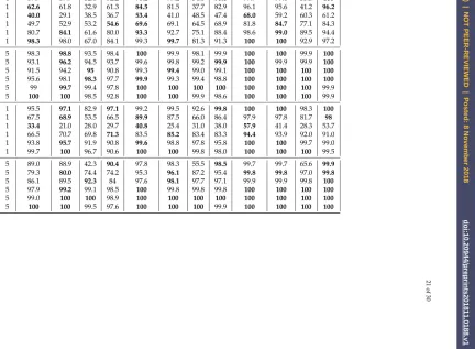
Table 10. Percentage of correct selections. DGP: SDM; Estimated equation SDM. T=1
CASE n=25 CASE n=49 CASE n=100
T ρ β1 θ Entropy Bayes MJ AIC Entropy Bayes MJ AIC Entropy Bayes MJ AIC
1 -0.8 1 1 53.3 54.0 35.7 57.7 67.0 68.3 28.3 70.6 80.7 79.8 34.2 81.9 1 -0.5 1 1 45.8 42.7 32.1 48.5 52.3 51.1 29.8 54.9 59.1 57.4 32.3 63.2 1 -0.2 1 1 33.7 33.2 34.9 38.2 36.0 30.9 32.9 34.7 30.8 25.0 30.2 33.0 1 0.2 1 1 24.3 23.1 35.7 25.5 29.5 18.3 37.1 28.1 37.9 18.6 37.6 34.9 1 0.5 1 1 27.8 23.3 41.6 27.6 45.2 33.5 46.1 40.6 63.4 57.1 42.1 60.7 1 0.8 1 1 36.8 31.1 40.7 33.4 62.8 61.7 53.4 55.1 80.5 82.3 55.0 67.3 1 -0.8 1 5 65.9 57.7 43.9 61.9 81.4 75.3 53.1 77.7 90.5 91.0 69.4 92.9 1 -0.5 1 5 55.0 53.5 45.5 57.2 67.4 71.5 55.3 72.6 81.4 83.9 71.1 84.3 1 -0.2 1 5 51.2 48.2 47.1 49.7 57.8 56.5 56.6 54.4 72.7 70.9 72.1 71.0 1 0.2 1 5 45.9 45.1 53.2 43.3 57.6 51.6 63.6 53.8 73.4 65.7 74.2 69.8 1 0.5 1 5 52.7 44.8 57.4 46.4 66.2 61.5 68.6 67.6 83.3 79.0 74.7 79.8 1 0.8 1 5 62.1 51.5 60.1 56.6 81.1 87.6 82.6 78.8 94.9 93.8 77.9 84.4 1 -0.8 5 1 59.8 57.7 42.6 62.2 75.8 74.8 46.4 76.6 84.0 85.7 55.3 88.2 1 -0.5 5 1 46.4 46.1 34.2 50.4 52.7 55.6 33.7 58.7 65.6 63.5 38.5 68.1 1 -0.2 5 1 34.7 31.0 31.9 36.2 28.5 28.6 29.1 33.0 28.6 22.3 26.9 32.5 1 0.2 5 1 29.0 27.4 41.3 30.1 31.9 23.4 44.8 30.9 46.7 26.9 45.8 39.4 1 0.5 5 1 39.6 35.7 49.3 37.5 55.7 48.7 58.1 55.1 74.6 70.3 59.2 69.8 1 0.8 5 1 58.0 49.1 55.2 50.6 76.7 85.7 78.2 76.0 93.3 92.0 73.9 81.3 1 -0.8 5 5 56.8 51.1 36.1 55.1 67.7 69.8 30.1 73.6 82.6 80.2 33.7 82.0 1 -0.5 5 5 48.1 47.1 34.9 51.1 56.6 56.4 39.6 59.0 70.6 70.2 49.5 73.6 1 -0.2 5 5 47.9 46.8 46.4 48.6 53.7 53.0 54.0 53.7 66.0 60.8 64.0 63.6 1 0.2 5 5 49.6 47.1 56.5 48.4 65.2 55.5 67.5 58.9 76.7 74.5 79.5 74.6 1 0.5 5 5 58.1 48.5 62.5 52.1 77.0 67.6 77.4 78.2 92.5 88.4 87.9 88.7 1 0.8 5 5 72.4 67.1 70.0 69.9 90.7 94.6 91.8 90.4 98.9 87.6 92.0 91.7
20
of
30
Table 11. Percentage of correct selections. DGP: SDM; Estimated equation SDM. T=5
Other parameters CASE n=25 CASE n=49 CASE n=100
T r b1 q1 Entropy Bayes MJ AIC Entropy Bayes MJ AIC Entropy Bayes MJ AIC
5 -0.8 1 1 75.4 77.0 30.7 78.3 92.2 92.6 35.2 93.9 98.2 98.2 33 99
5 -0.5 1 1 51.0 46.5 33.6 46.7 65.7 69.7 35.7 72.4 88.5 88.0 34.6 89.7 5 -0.2 1 1 34.4 22.6 34.1 26.9 38.3 30.4 40.1 37.7 51.3 39.7 45.8 48.5 5 0.2 1 1 41.5 33.8 39.6 41.1 53.9 49.5 51.7 55.8 71.3 67.1 63.0 48.5 5 0.5 1 1 68.5 66.9 48.2 64.6 80.7 82.0 64.1 74.9 92.6 93.7 76.7 88.6 5 0.8 1 1 88.3 89.1 52.4 72.9 97.1 96.5 72.2 79.6 99.7 99.5 81.8 91.1 5 -0.8 1 5 90.3 92.6 79.8 91.8 97.9 98.9 93.9 99.3 99.8 99.9 98.3 99.9 5 -0.5 1 5 84.6 85.8 82.2 79.5 96.6 96.7 94.7 97.0 99.7 99.6 99.3 99.8 5 -0.2 1 5 82.3 80.8 85.0 71.8 92.3 95.1 95.1 93.3 99.6 99.6 99.4 99.4
5 0.2 1 5 88.5 85.9 89.7 85.7 96.6 97.3 97.5 95.4 99.8 100 100 99.5
5 0.5 1 5 94.6 92.7 90.5 90.4 98.5 99.6 99.3 96.4 100 100 100 99.6
5 0.8 1 5 98.3 97.4 84.1 83.0 99.9 99.9 99.4 93.5 100 100 100 98.5
5 -0.8 5 1 85.3 89.1 70.3 89.5 96.0 96.4 79.6 98.0 99.4 99.4 91.3 99.8 5 -0.5 5 1 54.3 55.1 44.4 51.7 73.2 76.3 52.0 77.0 92.2 93.8 68.6 94.2 5 -0.2 5 1 27.9 17.6 27.0 24.5 30.0 18.3 28.9 31.8 39.1 25.7 29.3 39.3 5 0.2 5 1 56.4 45.6 53.1 51.3 66.1 66.6 68.8 69.1 83.7 85.5 84.1 82.6 5 0.5 5 1 83.5 83.3 79.2 83.5 93.0 95.8 92.9 89.0 98.3 98.8 97.8 95.8
5 0.8 5 1 97.5 97.8 78.5 81.7 99.7 99.7 98.5 89.5 100 100 100 97.9
5 -0.8 5 5 78.0 79.7 38.7 80.4 93.0 93.8 44.0 94.1 97.7 98.4 52.6 98.5 5 -0.5 5 5 67.2 66.6 61.8 60.8 83.3 87.2 72.4 87.6 96.9 96.7 85.3 97.1
5 -0.2 5 5 78.6 70.3 76.4 65.6 88.0 89.0 90.6 85.3 97.2 98 97.3 97.4
5 0.2 5 5 93.5 88.8 90.9 86.9 98.2 99.3 99.1 97.6 100 100 100 100
5 0.5 5 5 98.5 96.8 96.3 96.1 99.6 100 99.9 98.5 100 100 100 99.7
5 0.8 5 5 99.8 99.8 91.3 92.9 100 99.9 100 98.6 100 100 100 100
21
of
30
Table 12. Percentage of correct selections. DGP: SDM; Estimated equation SDM. T=10
Other parameters CASE n=25 CASE n=49 CASE n=100
T r b1 q1 Entropy Bayes MJ AIC Entropy Bayes MJ AIC Entropy Bayes MJ AIC
10 -0.8 1 1 89.7 89.9 32.8 92.2 98.2 97.2 34.0 98.6 99.7 99.6 35.3 100 10 -0.5 1 1 62.6 61.8 32.9 61.3 84.5 81.5 37.7 82.9 96.1 95.6 41.2 96.2 10 -0.2 1 1 40.0 29.1 38.5 36.7 53.4 41.0 48.5 47.4 68.0 59.2 60.3 61.2 10 0.2 1 1 49.7 52.9 53.2 54.6 69.6 69.1 64.5 68.9 81.8 84.7 77.1 84.3 10 0.5 1 1 80.7 84.1 61.6 80.0 93.3 92.7 75.1 88.4 98.6 99.0 89.5 94.4
10 0.8 1 1 98.3 98.0 67.0 84.1 99.3 99.7 81.3 91.3 100 100 92.9 97.2
10 -0.8 1 5 98.3 98.8 93.5 98.4 100 99.9 98.1 99.9 100 100 99.9 100
10 -0.5 1 5 93.1 96.2 94.5 93.7 99.6 99.8 99.2 99.9 100 99.9 99.9 100
10 -0.2 1 5 91.5 94.2 95 90.8 99.3 99.4 99.0 99.1 100 100 100 100
10 0.2 1 5 95.6 98.1 98.3 97.7 99.9 99.3 99.4 98.8 100 100 100 100
10 0.5 1 5 99 99.7 99.4 97.8 100 100 100 100 100 100 100 99.9
10 0.8 1 5 100 100 98.5 92.8 100 100 99.9 98.6 100 100 100 99.9
10 -0.8 5 1 95.5 97.1 82.9 97.1 99.2 99.5 92.6 99.8 100 100 98.3 100
10 -0.5 5 1 67.5 68.9 53.5 66.5 89.9 87.5 66.0 86.4 97.9 97.8 81.7 98 10 -0.2 5 1 33.4 21.0 28.0 29.7 40.8 25.4 31.0 38.0 57.9 41.4 28.3 53.7 10 0.2 5 1 66.5 70.7 69.8 71.3 83.5 85.2 83.4 83.3 94.4 93.9 92.0 91.0
10 0.5 5 1 93.8 95.7 91.9 90.8 99.6 98.8 97.8 95.8 100 100 99.7 99.0
10 0.8 5 1 99.7 100 96.7 90.6 100 100 99.8 98.0 100 100 100 99.5
10 -0.8 5 5 89.0 88.9 42.3 90.4 97.8 98.3 55.5 98.5 99.7 99.7 65.6 99.9 10 -0.5 5 5 79.3 80.0 74.4 74.2 95.3 96.1 87.2 95.4 99.8 99.8 97.0 99.8
10 -0.2 5 5 86.1 89.5 92.3 84 97.6 98.1 97.7 97.1 99.9 99.9 99.8 100
10 0.2 5 5 97.9 99.2 99.1 98.5 100 99.8 99.8 99.8 100 100 100 100
10 0.5 5 5 99.0 100 100 98.9 100 100 100 100 100 100 100 100
10 0.8 5 5 100 100 99.5 97.6 100 100 100 99.9 100 100 100 100