Permutation Entropy: New Ideas and Challenges

(1)

Permutation Entropy: New Ideas and Challenges

Karsten Keller1*, Teresa Mangold1, Inga Stolz1, and Jenna Werner1 Institute of Mathematics, University of Lübeck, Lübeck D-23562, Germany * Correspondence: [email protected]; Tel.: +49-451-3101-6030

Abstract: During the last years some new variants of Permutation entropy have been introduced and applied to EEG analysis, among them a conditional variant and variants using some additional metric information or being based on entropies different from the Shannon entropy. In some situations it is not completely clear what kind of information the new measures and their algorithmic implementations provide. We discuss the new developments and illustrate them for EEG data.

Keywords: ordinal patterns; Permutation entropy; Approximate entropy; Sample entropy; Conditional entropy of ordinal patterns; Kolmogorov-Sinai entropy; classification

1. Introduction

The concept of Permutation entropy introduced by Bandt and Pompe [1] in 2002 has been applied to data analysis in various disciplines (compare e.g. the collection [2], and [3], [4]). The Permutation entropy of a time series is the Shannon entropy of the distribution of ordinal patterns in the time series (see also [5]). Such ordinal patterns, describing order types of vectors, are coded by permutations. Denoting the set of permutations of{0, 1, . . . ,d}fordin the natural numbersNbyΠd,

we say that a vector(v0,v1, . . . ,vd)∈Rd+1hasordinal patternπ= (r0,r1, . . . ,rd)∈Πdif

vr0 ≥vr1. . .≥vrd−1 ≥vrd and

rl−1>rlifvrl−1 =vrl.

Definition 1. Theempirical Permutation entropy (ePE) of orderd ∈ Nandof delayτ ∈ Nof a time series(xt)N_t₌−₀1with N∈Nis given by

ePEd,τ,(xt)N_t₌−₀1

=−1 d_π

∑

_∈_Π

d pτ

πlnp τ

π, (1)

where

pτ

π=

#{t∈ {dτ,dτ+1, . . . ,N−1} |(xt,xt−τ, . . . ,xt−dτ)has ordinal patternπ}

N−dτ (2)

is the relative frequency of ordinal patterns π in the time series and 0 ln 0 is defined by 0. The vectors

(xt,xt−τ, . . . ,xt−dτ)related to t,d andτare calleddelay vectors.

In contrast to some other presentations of Permutation entropy in literature the defining formula contains the term 1_d. This is justified by an interesting statement shown by Bandt et al. [6], which is roughly saying that for time series from a special class of systems, for d → ∞, (1) approaches to a nonnegative real number, it is however open how large the corresponding class is. Some further discussion of this point is following in this paper.

(2)

measures of that type are the fine-grained Permutation entropy proposed by Liu and Wang [7], the weighted Permutation entropyand therobust Permutation entropyintroduced by Fadlallah et al. [8] and Keller et al. [9], respectively, Bian et al. [10] have adapted Permutation entropy to the situation of delay vectors with equal components which are relevant when the number of possible values in a time series is small. Other variants are to consider Tsallis or Renyi entropies instead of the Shannon entropy which goes back to the work of Zunino et al. [11] and Liang et al. [12], or to integrate information of different scales as done by Li et al. [13], Ouyang et al. [14] and Azami and Ascodero [15]. Unakafov and Keller [16] have proposed the Conditional entropy of (successive) ordinal patterns as a measure which has been shown to perform better than the Permutation entropy itself in many cases.

In this paper we discuss some of the new (‘non-weighting’) developments on Permutation entropy. We first give some theoretical background in order to justify and to motivate conditional variants of Permutation entropy. Then we have a closer look at Renyi and Tsallis modifications of Permutation entropy. The last part of the paper is aimed to the classification of data from the viewpoint of epileptic activity. Here we point out that ordinal time series analysis combined with other methods and automatic learning could be promising for data analysis. We rely on EEG data reported in [17] and [18] and use algorithms developed in Unakafova and Keller [19].

2. Some theoretical background

The Kolmogorov-Sinai entropy.In order to get a better understanding of Permutation entropy, we take a modelling approach. For this, we choose a discrete dynamical system defined on a probability space(Ω,B,P). The elementsω∈Ωare considered as the (hidden) states of the system, the elements of theσ-algebraBas the events one is interested in, and the probabilityPmeasures the chances of such events taking place. The dynamics on the system is given by a mapT: Ω ←-being B − B-measurable, i.e. satisfyingT−1₍_B₎_{∈ B}_{for all}_B_{∈ B}_{. The map}_T_{is assumed to be}_P_-invariant

saying thatP(T−1(A)) = P(A)for allB ∈ Bin order to guarantee that the distribution of the states of the system does not change under the dynamics.

For simplicity, during the whole paper we assume that(Ω,B,P)and T are fixed; specifications are given directly where they are needed.

In dynamical systems the Kolmogorov-Sinai entropy based on entropy rates of finite partitions is a well established theoretical complexity measure. For explaining this concept, consider a finite partitionC =_{C1,C2, . . . ,Cl} ⊂ Band note that the (Shannon) entropy of such a partition is defined

by

H(_C) =₋

l

∑

i=1

P(Ci)lnP(Ci).

ForA= _{1, 2, . . . ,l}the setAkof wordsa1a2. . .akof lengthkoverAprovides a partitionCkof

Ωinto pieces

Ca1a2...ak :={ω∈Ω|(ω,T(ω), . . . ,T◦

k−1₍

ω))∈Ca1 ×Ca2×. . .×Cak}.

(In this paper T◦l _{denotes the} _l_{-fold concatenation of} _T_{, where} _T◦0 _{is the identity map.)} _The

distribution of word probabilitiesP(Ca1a2...ak) contains some information on the complexity of the system, which, as the word lengthkapproaches to∞, provides theentropy rate

EntroRate(_C) = lim

k→∞

1

kH(Ck) =klim→∞(H(Ck)−H(Ck−1)) (3)

ofC. The latter can be interpreted as the mean information per symbol. Here letH(C0) := 0. Note

(3)

In order to have a complexity not depending only on a fixed partition and measuring the overall complexity, theKolmogorov-Sinai entropy(KS entropy) is defined by

KS= sup

Cfinite partition

EntroRate(_C).

For more information, in particular concerning formula (3), see for example Walters [20].

By the nature of the concept of KS entropy, it is not easy to determine and to estimate from time dependent measurements of a system. One important point is to find finite partitions supporting as much information on the dynamics as possible. If there is no feasible so-calledgenerating partition containing all information (for a definition, see Walters [20]), this is not easy. The approach of Bandt and Pompe builds up appropriate partitions based on the ordinal structure of a system. Let us explain the idea in a general context.

Observables and ordinal partitioning.In the modeling, an observed time seriesx0,x1, . . . ,xN−1

is considered as the sequence of ‘outcoming’ valuesX(ω),X(T(ω)), . . .X(T◦N−1(ω))for someω ∈ Ω, whereX is a real-valued random variable on(Ω,B,P). HereX is interpreted as an observable establishing the outreading process.

Since it is no additional effort to consider more than one observable, letX= (X1,X2, . . . ,Xn) :

Ω → Rn be a random vector with observables X1,X2, . . . ,Xn as components. Originally, Bandt

and Pompe [1] discussed the case that the measuring values are coinciding with the states of a one-dimensional system, which in our language means thatΩ ⊂ R,n = 1, and there is only one observable which coincides with the identity map.

For each orderd∈Nwe are interested in the partition CX₍_d_{) =}_{_C

(π1,π2,...,πn)|πiordinal pattern fori=1, 2, . . . ,n} with

C₍_π₁_,_π₂_,...,_π_n₎=_{ω∈Ω|(Xi(T◦d(ω)), . . . ,Xi(T(ω)),Xi(ω))

has ordinal patternπifori=1, 2, . . . ,n}

calledordinal partition of order d. Here ordinal patterns are of orderdand the delay is one.

No information loss. For the rest of this section assume that the measurements by the observables do not loose information on the modelling system roughly meaning that the random variablesX1,X1◦T,X1◦T◦2, . . . ,X2,X2◦T,X2◦T◦2, . . . ,Xn,Xn◦T,Xn◦T◦2, . . . separate states ofΩ

and, more precisely, that for each eventCin theσ-algebra generated by these random variables there exists someB ∈ BwithP(C∆B) =0. Note that already for one observable the separation property described is mostly satisfied in a certain sense (see Takens [21], Gutman [22]).

Moreover, assume thatT isergodicmeaning thatP(T−1(B)) = P(B)impliesP(B) ∈ {0, 1}for allB ∈ B. Ergodicity says that the given system does not separate into proper subsystems and, by Birkhoff’s ergodic theorem (see [20]), allows to estimate properties of the system on the base of orbits ω,T(ω),T◦2(ω), . . ..

Under these assumptions it holds

KS= lim

d→∞EntroRate(C

X₍_d_{)) =}_sup

d∈N

EntroRate(_CX(d)). (4)

(4)

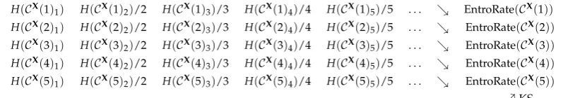
H(_CX₍₁₎

1) H(CX(1)2)/2 H(CX(1)3)/3 H(CX(1)4)/4 H(CX(1)5)/5 . . . & EntroRate(CX(1))

H(_CX₍₂₎

H(_CX(3)1) H(CX(3)2)/2 H(CX(3)3)/3 H(CX(3)4)/4 H(CX(3)5)/5 . . . & EntroRate(CX(3))

H(_CX₍₄₎

H(_CX₍₅₎

. . .%KS

Figure 1.Approximation of KS entropy: the direct way

Formula (4) to be read together with formula (3) is illustrated by Figures1and2, where directions of arrows indicate the direction of convergence.

Conditional entropy of ordinal patterns. In order to motivate a complexity measure based on considering successive ordinal patterns, we deduce some useful inequalities from the above statement. First fix somed∈Nand note that, since(H(CX(d)k)−H(CX(d)k−1))∞k=1is monotonically

non-increasing, it holds for allk∈N

H(_CX(d)_k)₋H(_CX(d)_k₋₁) _≤ 1 k

k

∑

i=1

(H(_CX(d)_i)₋H(_CX(d)_i₋₁))

= 1 kH(C

X₍_d₎

k).

Because EntroRate(_CX(d)) is converging to the KS entropy in a monotonically non-decreasing way, the following inequality is valid:

KS≤lim inf

d→∞ (H(C

X₍_d₎

kd)−H(C X₍_d₎

kd−1))≤lim inf_d →∞

1 kd

H(_CX(d)_k_d)

for each each sequence(kd)∞d=1of natural numbers.

Note that the faster the sequence(kd)∞d=1increases, the nearer are the terms in the inequality, and

good choices of the sequence provide equality of all terms in the last inequality. In particular, it holds

KS≤lim inf

d_→∞ (H(C

X₍_d₎

2)−H(CX(d))),

being the background for the following definition (compare Unakafov and Keller [16]):

Definition 2. H(_CX(d)2)−H(CX(d))is called theConditional entropy of ordinal patternsof order d.

Indeed the concept given is a conditional entropy, since howeverCX₍_d₎

2is a finer partition than CX₍_d₎_{, it reduces to a difference of entropies.}

Permutation entropy.The description of KS entropy given by formula (4) includes a double-limit where the inner one is non-increasing and the outer is non-decreasing. Bandt et al. [6] (see also [1])

H(_CX(1)2)−H(CX(1)1) H(CX(1)3)−H(CX(1)2) H(CX(1)4)−H(CX(1)3) . . . & EntroRate(CX(1))

H(_CX₍₂₎

2)−H(CX(2)1) H(CX(2)3)−H(CX(2)2) H(CX(2)4)−H(CX(2)3) . . . & EntroRate(CX(2))

H(_CX₍₃₎

H(CX₍₄₎

H(_CX(5)2)−H(CX(5)1) H(CX(5)3)−H(CX(5)2) H(CX(5)4)−H(CX(5)3) . . . & EntroRate(CX(5))

. . .%KS

(5)

have proposed the concept of Permutation entropy only needing one limit and being the starting point of using ordinal pattern methods. Here it is given in our general context.

Definition 3. For d ∈ N, the quantity PEX(d) = d1H(CX(d)) is called the Permutation entropy of

order d with respect to X. Moreover, by the Permutation entropy with respect toXwe understandPEX = lim sup_d_→_∞PEX(d).

The definition of Permutation entropy given is justified by the result of Bandt et al. [6] that ifT is a piecewise monotone interval map, then it holds PEid = KS. HereΩis an interval and X = id, whereiddenotes the the identity onΩ. We don’t want to say more about this result, but mention that general equality of KS entropy and Permutation entropy is an open problem, however as shown in [23] (under the assumptions above) it holds

KS≤PEX.

Assuming that the increments of entropy of successive ordinal partitions are well-behaved in the sense that

lim

d_→∞(H(C

X₍_d₊₁₎₎₋_H₍_CX₍_d₎₎₎ exists, by the Stolz-Cesàro theorem one obtains the inequality

KS ≤ lim inf

d→∞ (H(C

X₍_d₎

2)−H(CX(d)))

≤ lim

d→∞(H(C

X₍_d₊₁₎₎₋_H₍_CX₍_d₎₎₎ = lim

d→∞(H(C

X₍_d₎₎₋_H₍_CX₍_d₋₁₎₎₎

= lim

d→∞

1 d

d

∑

i=1

(H(CX₍_i₎₎₋_H₍_CX₍_i₋₁₎₎₎

= lim

d→∞

1 dH(C

X₍_d_{)) =}_PEX

(compare [16]). This inequality is shading some light on the relationship of KS entropy, Permutation entropy and the various conditional entropy differences (see Figure2) considered.

Summarizing, all quantities we have considered are related to the entropies H(_CX(d)_k). For simplicity, we now switch to only one observableX. The generalization is simple but not necessary for the following. In the restricted case, ford,k∈Nit holds

H(_CX(d)_k) =₋

∑

(πl)kl=1∈Πkd

P₍_π

l)kl=1lnP(πl)kl=1,

where

P

(π_l)k l=1

=P(_{ω∈Ω|(X(T◦l+d−1(ω)), . . . ,X(T◦l(ω)),X(T◦l−1(ω))) has ordinal patternπlforl=1, 2, . . . ,k}).

(6)

ofP(_CX(d)_k)from orbits of a system whendorkis high. Here forn,k∈Na naive estimator ofP₍_π l)kl=1

is

p₍_π l)kl=1

= #{t∈ {d+k−1, . . . ,N−1} |(xt−i, . . . ,xt−i−d)has ord. patt.πifori=0, . . . ,k−1} N−d−k+1

and a naive estimator ofH(CX₍_d₎ k)is

h(d,k) =−

∑

(πl)kl=1∈Πkd

p₍_π

l)kl=1lnp(πl)kl=1.

The problem is that one needs too many measurements for a reliable estimation ifd andkare large. This is demonstrated in the one dimensional case for the logistic map with ‘maximal chaos’. HereΩ= [0, 1],Tis defined byT(ω) =4ω(1−ω)forx ∈[0, 1],Pis the Lebesgue measure, andXis the identity map. Note that this map and maps of the whole logistic family are often used for testing complexity measures. (For more information, see [25] and [26].)

102 103 104 105

0 0.1 0.2 0.3 0.4 0.5 0.6 0.7 0.8

102 ₁₀3 ₁₀4 ₁₀5 ₁₀6

-0.1 0 0.1 0.2 0.3 0.4 0.5 0.6 0.7

102 ₁₀3 ₁₀4 ₁₀5

0 0.2 0.4 0.6 0.8 1

h(4,2)−h(4,1) h(5,2)−h(5,1) h(6,2)−h(6,1) h(7,2)−h(7,1) h(2,2)−h(2,1) h(3,2)−h(3,1)

h(7,1)/7 h(6,1)/6 h(5,1)/5

h(7,6)−h(7,5)

h(7,5)−h(7,4)

h(7,4)−h(7,3)

h(7,3)−hh(7(7,,2)2)−h(7,1)

h(7,7)−h(7,6)

h(7,8)−h(7,7)

h(7,9)−h(7,8)

h(7,10)−h(7,9)

Figure 3. Different estimates of the KS entropy ofT(ω) = 4ω(1−ω);ω ∈ [0, 1]for different orbit

lengths. On the top: h(d, 2)₋h(d, 1)ford = 2, 3, . . . , 7; in the middle: h(7,k)₋h(7,k−1)fork =

2, 3, . . . , 10; on the bottom:h(d, 2)−h(d, 1)versush(d_d,1) ford=5, 6, 7.

(7)

compromise. Good performance of Conditional entropy of ordinal patterns for the logistic family is reported in Unakafov and Keller [16].

3. Generalizations based on the families of Renyi and Tsallis entropies

The concept. It is natural to generalize Permutation entropy to Tsallis and Renyi entropy variants, which has first been done by Zunino et al. [11]. Liang et al. [12] discuss performances of a large list of complexity measures, among them the classical as well as Tsallis and Renyi Permutation entropies in tracking changes of EEG during different anesthesia states. They report that the class of Permutation entropies in some features show good performance relative to the other measures, with best results for the Renyi variant. Let us have a closer look at the new concepts.

Definition 4. For some given positive α 6= 1, the empirical Renyi Permutation entropy (eRPE) and empirical Tsallis Permutation entropy (eTPE)oforderd∈Nand ofdelayτ∈Nof a time series(xt)_tN₌−₀1

with N∈Nis defined by

eRPEα,d,τ,(xt)N_t₌−₀1

=₋ 1

d(1−α)ln

∑

π∈Πd

(pτ π)α

and

eTPEα,d,τ,(xt)N_t₌−₀1

=₋ 1

d(α−1) 1−

∑

π∈Πd

(pτ π)α

!

,

respectively, with pπas given in(2). (We include the factor 1_d into the entropy formulas only for reasons of

comparability with the classical Permutation entropy.)

Some properties. As in general the Renyi and the Tsallis entropy of a distribution for α → 1 converge to the Shannon entropy, convergence of eRPE and eTPE to the ePE holds. The two concepts principally can be used in data analysis to more emphasize the role of small ordinal pattern probabilities ifα<1 or of large ones ifα>1 (compare the graphs of the functionsx 7→xlnx, x 7→xα for differentαandx ∈ [0, 1]). The consequences of this weighting gets obvious for the eRPE when considering limits forα→0 andα→∞. One easily sees that

lim

α→∞eRPE

α,d,τ,(xt)N_t₌−₀1

= ₋ln(maxπ∈Πd p

τ π)

d lim

α→0eRPE

α,d,τ,(xt)N_t₌−₀1

= ln(#{π∈Πd| p

τ π6=0})

d ,

meaning that for largeαthe eRPE mainly measures the largest relative ordinal pattern frequency, with low entropy for high relative frequency, and for smallαthe number of occurring ordinal patterns. Since

eTPEα,d,τ,(xt)Nt=−01

= e

d(1−α)eRPE(α,d,τ,(xt)Nt=−01)−₁

d(1−α) ,

the eTPE is only a monotone functional of the eRPE for fixed α; despite of a different scale it has similar properties as the eRPE.

For α = 2 the eRPE has a nice interpretation. Having Nπ = (N−dτ)pτπ in the time series,

then there are Nπ(Nπ−1)

2 pairs of different times providing ordinal patternπ. Since all in all we have

(N−dτ)(N−dτ−1)

2 different time pairs, the quantity

∑π∈ΠdNπ(Nπ−1)

(N−dτ)(N−dτ−1) =

∑π∈Πd N 2

π−(N−dτ)

(N−dτ)2−(N−dτ) ≈_π

∑

_∈_Π d

(pτ π)

(8)

0 20 40 60 80 100 0.7

0.8 0.9 1.0

0 20 40 60 80 100

0.5 0.6 0.7 0.8 0.9 1.0

0 20 40 60 80 100

0.4 0.5 0.6 0.7 0.8 0.9 1.0

0 20 40 60 80 100

0.22 0.24 0.26 0.28 0.30 0.32

0 20 40 60 80 100

0.85 0.90 0.95 1.00 1.05

0 20 40 60 80 100

0.6 0.7 0.8 0.9 1.0

0 20 40 60 80 100

0.4 0.5 0.6 0.7 0.8 0.9 1.0

0 20 40 60 80 100

0.24 0.26 0.28 0.30 0.32

data set 2, eTPE,α=2

data set 2, eRPE,α=2

data set 2, ePE data set 2, eRPE,α=0.5 data set 1, eTPE,α=2

data set 1, eRPE,α=2 data set 1, ePE data set 1, eRPE,α=0.5

seconds

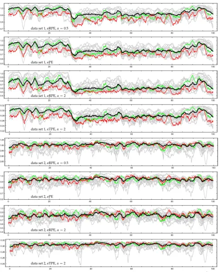
Figure 4. Comparison of eRPE for α = 0.5, 2, eTPE for α = 2 and ePE, computed from EEG

recordings before stimulator implantation (data set 1) and after stimulator implantation (data set 2) for 19 channels using a shifted time window, orderd=3 and delayτ=4. Highlighting, in particular,

(9)

0 20 40 60 80 100 0.009803921567

0.009803921568

0 20 40 60 80 100

0.2 0.4 0.6 0.8 1.0

0 20 40 60 80 100

0.85 0.90 0.95 1.00 1.05

seconds data set 1, eTPE,α=35

data set 1, eRPE,α=35

data set 1, eRPE,α=0.01

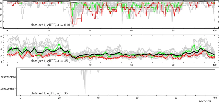
Figure 5.eRPE forα=0.01, 35 and eTPE forα=35 computed from data set 1 for 19 channels using a

shifted time window,d=3 andτ=4 (cf. Figure4).

Table 1.Concordance of sign of entropy differences of ePE and eRPE for givenα

α 0.5 0.8 0.9 1.1 1.2 1.5 2 250

Fp2 98.69 % 99.52 % 99.77 % 99.78 % 99.58 % 99.05 % 98.38 % 94.85 %

T3 95.41 % 98.39 % 99.22 % 99.26 % 98.59 % 96.92 % 95.20 % 89.31 %

P3 93.18 % 97.71 % 98.93 % 99.05 % 98.21 % 96.30 % 94.33 % 83.66 %

can be interpreted as the degree of recurrence in the time series. This quantity is in fact thesymbolic correlation integralrecently introduced by Caballero et al. [27].

Demonstration.We demonstrate the performance of eRPE and eTPE for differentαon the base of EEG data discussed in [17]. For this, we consider two parts each of a 19-channel scalp EEG of a boy with lesions predominantly in the left temporal lobe caused by a connatal toxoplasmosis. The data were sampled with a rate of 256 Hz, meaning that 256 measurements were obtained each second. The first data part (data set 1) was taken from an EEG derived at an age of eight years and the second one (data set 2) was derived at an age of 11 years, four months after the implantation of a vagus stimulator. Note that epileptic activity was significant before vagus stimulatation and was the reason for the implantation. (For some more details on the data, see [17]).

Figure4shows ePE, eRPE forα=0.5, 2 and eTPE forα=2 for the two data sets in dependence on a shifted time window, whered = 3 andτ = 4. Each graphic represents the 19 channels for a fixed entropy by 19 entropy curves. Among the channels areT3and P3, which are interesting in the following. The curve related to a fixed channel contains pairs (t,ht), whereht is the entropy

of the segment of the related time series ending at timet and containing 2·256+3·4 successive measurements. (Each segment provides 512=2·256 ordinal patterns representing a time segment of two seconds.) Thetare chosen from a time segment of 100 seconds, where the beginning time is set to 0 for simplicity. We have added a fat black curve representing the entropy of the whole brain instead of the single channels. Here the relative frequencies used for entropy determination were obtained by counting ordinal patterns in the considered time segment pooled over all channels.

(10)

considered. Here we want to note thatP3andT3are from the left part of the brain with the lesions, and mainlyP3seems to reflect some kind of irregular behavior related to them. The most interesting point is that before vagus stimulator implantationP3and partiallyT3are conspicuous both in phases with and without epileptic activity. For orientation: The graphic given in Figure4for data set 1 and in Figure5show a part from around 30 to 90 seconds with low entropies for pooled ordinal patterns (fat black curve) related to a generalized epileptic seizure meaning epileptic activity in the whole brain.

Figure4suggests that a visual inspection of the data using eRPE and eTPE instead of ePE does not seem to get further insights whenαis chosen close to 1. Here it is important to note that, for the parameters considered, all ordinal patterns are accessed at many times (with some significant frequency). Our guess is supported by Table1. For each of the channels FP2,T3, andP3and givenα, the relative frequency of concordant pairs of the observations ePE, eRPE at timesand ePE, eRPE at timetamong all pairs(s,t);s < tis shown. (s,t)is said to be concordant if the difference between ePE at timessandtand the difference between eRPE at timessandthave the same sign.

The results particularly reflect the fact that for channel Fp2, providing measurements from the front of the brain, the ordinal patterns are more equally distributed than forT3, as well as that for P3 the distribution of ordinal patterns is the farthest from equidistribution. For contrast, we also considerα = 250. Figure5related to data set 1 indicates that extreme choices ofαcould be useful in order to analyze and visualize changes in the brain dynamics more forceful. The upper graphic of eRPE forα=0.01 shows that at the beginning of an epileptic seizure the number of ordinal patterns abruptly decreases for nearly all channels and, after some increasing, stays on a relatively low level until the end of the seizure. Forα=35 it is interesting to look at the whole ensemble of the entropies. Here eRPE indicates much more variability of largest ordinal pattern frequencies of the channels in the seizure-free parts than in the seizure epochs. The very low entropy at the beginning of the seizure mainly goes back to much more only increasing or decreasing ordinal patterns. Here the special kind of scaling given by the eTPE allows to emphasize the special situation at the beginning of a seizure and can therefore be interesting for an automatic detection of epileptic seizures, whereby a right tuning ofαis important.

4. Classification on the base of different entropies

Classification is an important issue in the analysis of EEG data, for which in many cases entropy measures can be exploited. Here often it is not clear which of these measures are the best and how much they are ‘overlapping’. In view of the discussion in Section2, we note that although the nature of Shannon entropy based measures, which we considered in this paper, is nearly similar for low orders, their performance can be rather different in dependence on the delay.

Here we want to discuss classification of EEG data using ePE, empirical Conditional entropies of ordinal patterns (eCE, see below) and, additionally, Approximate entropy (AppEn) (see Pincus [28]) and Sample entropy (SampEn) (see Richmann and Moormann [29], and extending work in Keller et al. [9]). For definition and usage of AppEn and SampEn, in particular for the parameter choice ("AppEn(2, 0.2σ,x)", "SampEn(2, 0.2σ,x)"), we directly refer to [9]. The eCE, motived and defined for dynamical systems in Section2, is given by the following definition (compare also [9]):

Definition 5. Given a time series(xt)Nt=−01with N∈N, the quantity

eCEd,τ,(xt)_tN₌−₀1

=

∑

π∈Πd pτ

πlnpτπ−

∑

π1,π2∈Πd pτ

(11)

Figure 6.Entropy of the EEG data sorted by groups for four differnt entropy measures

is calledempirical Conditional entropy of ordinal patterns (eCE)oforderd ∈ Nand ofdelayτ ∈ N, where pτ

πis defined by(2)and pτπ1,π2by

pτ π1,π2 =

1

N−dτ−1#{t∈ {dτ,dτ+1, . . . ,N−2} |

(xt,xt−τ, . . . ,xt−dτ),(xt+1,xt+1−τ, . . . ,xt+1−dτ)have ordinal patternsπ1,π2}

Note that for each time series(xt)N_t₌−₀1and eachd ∈ N, it holds eCE

d, 1,(xt)_tN₌−₀1

=h(d, 2)₋ h(d, 1). So eCEd, 1,(xt)N_t₌−₀1

is an estimate of the Conditional entropy of ordinal patterns defined in Section2.

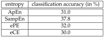
Table 2.Results for classification on the base of one entropy

entropy classification accuracy (in %)

ApEn 31.0

SampEn 37.8

ePE 32.0

eCE 30.0

(12)

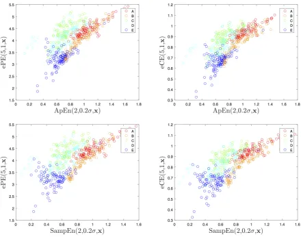
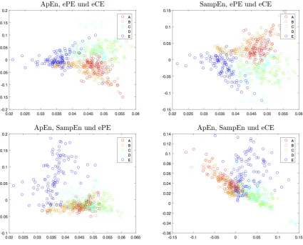
Figure 7.One entropy versus another one for four entropy combinations

• group A:surface EEG’s recorded from healthy subjects with open eyes, • group B:surface EEG’s recorded from healthy subjects with closed eyes,

• group C:intracranial EEG’s recorded from subjects with epilepsy during a seizure-free period from within the epiloptogenic zone,

• group D:intracranial EEG’s recorded from subjects with epilepsy during a seizure-free period from hippocampal formation of the opposite hemisphere of the brain,

• group E:intracranial EEG’s recorded from subjects with epilepsy during a seizure period. In contrast to [9], where the groups A and B and the groups C and D were pooled, each of the groups is considered separately in the following.

Table 3.Results for classification on the base of two entropies

entropy classification accuracy (in %)

ApEn & SampEn 51.0

ApEn & ePE 58.0

ApEn & eCE 61.8

SampEn & ePE 64.0

SampEn & eCE 64.6

ePE & eCE 48.2

(13)

Figure 8. Second principal component versus first one obtained from principal component analysis on three entropy variables

obtained are drawn from the left to the right starting from those from group A and ending with those from group E. One sees that each of the considered entropies is not much separating, however, one can see different kinds of separation properties for the ordinal pattern based entropies and the two other entropies. A better separation is seen in Figure7where one entropy measure is plotted versus another one, in four different combinations. Here the discrimination between E, the union of A and B, and the union of C and D is rather good, confirming the results in [9], but bothA,BandC,Dare strongly overlapping. The general separation seems to be slightly better using three entropies, which is illustrated by Figure8. Here, however, a two-dimensional representation is chosen by plotting the second principal component versus the first one, both obtained by principal component analysis from the three entropy components variables.

Table 4.Results for classification on the base of three entropy

entropy classification accuracy (in %) ApEn & SampEn & ePE 67.4

ApEn & SampEn & eCE 66.8 ApEn & ePE & eCE 65.4 SampEn & ePE & eCE 71.8

(14)

of 80% of the data sets and a testing group consisting of the remaining 20%. The obtained accuracy of the classification, i.e. the relative frequency of correctly classified data sets, was averaged over 1000 testing trials for each entropy combination considered. The results of this procedure, summarized in Tables2,3and4, show that including a further entropy results in a higher accuracy, but that the way of combining entropies is crucial for the results. Note that combining all four entropies provides an accuracy of only 70.6%.

Clearly, accuracy of classification using ePE and eCE depends on the choice of the parameters of the entropies. Whereas the choice of higher orders doesn’t make sense by statistical reasons as already mentioned in Section2, testing different delaysτis useful since the delay contains important scale information. Note that already for both, ePE and eCE, the classification accuracy varies by more then 14%. Considering only delaysτ=1, 2, . . . , 9 ford=5, the maximal accuracies for ePE and eCE is 45.01% and 48.0% forτ=6 andτ=5, respectively. Note that both results are better than those for the SampEn (see Table2) and thatτ=1 provides the worst results. Combining two ePE’s and eCE’s for delays, in{1, 2, . . . , 9}one reaches accuracy of 61.79% (for delays 1 and 2) and 62.28% (for delays 1 and 9), respectively.

5. Resume

Throughout this paper, we have discussed ordinal pattern based complexity measures both from the viewpoint of their theoretical foundation and their application in EEG analysis, in the center the Permutation entropy and conditional variants of it. We have pointed out that, as in many situations in (model-based) data analysis, one has to attract attention to the discrepancy of theoretical asymptotics and statistical requirements, here in view of estimating KS entropy. In the case of moderately but not extremely long data sets, the concept of Conditional entropy of ordinal patterns as discussed could be a compromise. It has been shown to have a better performance than the classical Permutation entropy in many situations.

A good way of further investigating performances of ordinal pattern based measures is an extensive testing of these measures for data classification. In this direction, the results of this paper for a restricted parameter choice are already promising, however further studies are required. For this manner, based on the considerations in Sections 4 and 3, the authors also propose including Renyi and Tsallis variants of Permutation entropy (with an extreme parameter choice) and classical concepts like Approximate entropy and Sample entropy. The latter are interesting in combination with ordinal complexity measures since they possibly address other features. The most important challenge, however, is to deal with the great number of entropy measures and parameters, in the opinion of the authors this can be faced by using machine learning ideas in a sophisticated way.

Acknowledgements

We would like to thank Heinz Lauffer from the Clinic and Outpatient Clinic for Pediatrics of the University Greifswald for providing the EEG data discussed in Section3. Moreover, the first author thanks Manuel Ruiz Marín from the Technical University of Cartagena and his colleagues for some nice days in South Spain discussing their concept of Symbolic correlation integral.

Conflicts of Interest

The authors declare no conflict of interest.

Bibliography

(15)

2. Amigó, J.M.; Keller, K; Kurths, J. (eds) Recent progress in symbolic dynamics and permutation complexity. Ten years of permutation entropy.Eur. Phys. J. Spec. Top.2013,222, 247—257.

3. Zanin, M.; Zunino, L.; Rosso, O.A.; Papo, D. Permutation entropy and its main biomedical and econophysics applications: A review.Entropy2012,14, 1553-1577.

4. Amigó J.M.; Keller, K.; Unakafova, V.A. Ordinal symbolic analysis and its application to biomedical recordings.Phil. Trans. Royal. Soc. A,2015,373, 20140091.

5. Amigó, J.M.Permutation Complexity in Dynamical Systems. Springer-Verlag: Berlin-Heidelberg, 2010. 6. Bandt, C.; Keller, G.; Pompe, B. Entropy of interval maps via permutations. Nonlinearity 2002, 15(5),

1595–1602.

7. Liu, X-F.; Wang, Y. Fine-grained permutation entropy as a measure of natural complexity for time series. Chin. Phys. B2009,18, 2690–2695.

8. Fadlallah, B.; Chen, B; Keil, A; Príncipe, J. Weighted-permutation entropy: A complexity measure for time series incorporating amplitude information.Phys. Rev. E2013,87, 022911.

9. Keller, K.; Unakafov, A.M.; Unakafova, V.A. Ordinal Patterns, Entropy, and EEG. Entropy 2014, 16, 6212-6239.

10. Bian, C.; Qin, C.; Ma, Q.D.Y.; Shen, Q. Modified permutation-entropy analysis of heartbeat dynamics.Phys. Rev. E2012,85, 021906.

11. Zunino, L.; Perez, D.G.; Kowalski, A.; Martín, M.T.; Garavaglia, M.; Plastino, A.; Rosso, O.A. Brownian motion, fractional Gaussian noise, and Tsallis permutation entropy.Physica A2008,387, 6057–6068. 12. Liang, Z; Wang, Y.; Sun, X.; Li, D.; Voss, L.J.; Sleigh, J.W.; Hagihira, S.; Li, X. EEG entropy measures in

anesthesia.Front. Comput. Neurosci.2015,9, 00016.

13. Li, D.; Li, X.; Liang, Z.; Voss, L.J.; Sleigh, J.W. Multiscale permutation entropy analysis of EEG recordings during sevoflurane anesthesia.J. Neural Eng.2010,7, 046010.

14. Ouyang, G.; Li, J.; Liu, X.; Li, X. Dynamic characteristics of absence EEG recordings with multiscale permutation entropy analysis.Epilepsy Res.,2013,104, 246–252.

15. Azami, H.; Escudero, J. Improved multiscale permutation entropy for biomedical signal analysis: Interpretation and application to electroencephalogram recordings.Biomed. Signal Proces.2016,23, 28–41. 16. Unakafov, A.M.; Keller, K. Conditional entropy of ordinal patterns.Physica D2013,269, 94–102.

17. Keller, K.; Lauffer, H. Symbolic analysis of high-dimensional time series. Int. J. Bifurc. Chaos 2003, 13, 2657–2668.

18. Andrzejak, R.G.; Lehnertz, .K; Rieke, C.; Mormann, F; David, P; Elger, C.E. Indications of nonlinear deterministic and finite dimensional structures in time series of brain electrical activity: Dependence on recording region and brain state.Phys. Rev. E2001,64, 061907.

19. Unakafova, V.A.; Keller, K. Efficiently Measuring Complexity on the Basis of Real-World Data.Entropy2013, 15, 4392–4415.

20. Walters, P.An Introduction to Ergodic Theory. Springer-Verlag: New York, 1982.

21. Takens, F. Detecting strange attractors in turbulence. in: “Dynamical Systems and Turbulence” (eds.: Rand, D.A.; Young, L.S.),Lecture Notes in Mathematics 898, Springer-Verlag: Berlin-New York, 1981, 366-381. 22. Gutman, J. Takens’ embedding theorem with a continuous observable. preprint, math/1510.05843. 23. Antoniouk, A.; Keller, K.; Maksymenko, S. Kolmogorov-Sinai entropy via separation properties of

order-generatedσ-algebrasDiscrete Contin. Dyn. Syst. A2014,34, 1793–1809.

24. Keller, K.; Maksymenko, S., Stolz, I. Entropy determination based on the ordinal structure of a dynamical system.Discrete Contin. Dyn. Syst. B2015,20, 3507–3524.

25. Sprott, J.C.Chaos and time-series analysis. Oxford University Press: Oxford, 2003.

26. Young, L.-S. Mathematical theory of Lyapunov exponents.J. Phys. A: Math. Theor.2013,46, 1–17.

27. Caballero, M.V.; Mariano, M.; Ruiz, M. Draft: Symbolic correlation integral. Getting rid of the proximity parameter,http://data.leo-univ-orleans.fr/media/seminars/175/WP_208.pdf(accessed: 14-Feb-2017). 28. Pincus, S.M. Approximate entropy as a measure of system complexity. Proceedings of the National Academy

of Sciences1991,88, 2297–2301.

29. Richman, J.S.; Moorman, J.R. Physiological time-series analysis using approximate entropy and sample entropy.American Journal of Physiology-Heart and Circulatory Physiology2000,278, 2039–2049.

(16)

c