Mathematical Modelling of Human African Trypanosomiasis using Control Measures

Mathematical Modelling of Human African Trypanosomiasis

using Control Measures

Hamenyimana Emanuel Gervas

, Nicholas Opoku

, Shamsuddeen Ibrahim

1_{African Institute for Mathematical Sciences, Ghana.} 2_{University of Cape Coast, Ghana.}

1_{To whom correspondence should be addressed; E-mail: [email protected]}

Abstract

Human African Trypanosomiasis (HAT) commonly known as sleeping sickness, is a neglected tropical vector borne disease caused by trypanosome protozoa. It is transmitted by bites of infected tsetse fly. In this paper we first present the vector-host model which describes the general transmission dynamics of HAT. In the tsetse fly population, the HAT is modelled by three compartments while in the human population, the HAT is modelled by four compartments. The next generation matrix approach is used to derive the basic reproduction number,R0,

and also it is proved that ifR0 ≤1the disease free equilibrium is globally asymptotically stable, which means

the disease dies out. The disease persist in the population if the value ofR0>1. Furthermore, the optimal

con-trol model is determined by using the Pontryagin’s maximum principle with concon-trol measures such as education, treatment and insecticides used to optimize the objective function. The model simulations confirm that the use of the three control measures are very efficient and effective to eliminate HAT in Africa.

Keywords:Human African Trypanosomiasis (HAT), Mathematical modelling, optimal control, Control mea-sures.

1

Introduction

Human African trypanosomiasis (HAT), commonly known as sleeping sickness, is a vector-borne tropical disease which is caused by trypanosoma brucei protozoa species. It is one of the neglected tropical diseases which affects people in sub-Saharan Africa specifically those living in rural areas. HAT is caused by two species of protozoa which are Trypanosoma brucei gambiense (TBG), which causes the chronic form of HAT in central and western Africa and Trypanosoma brucei rhodesiense (TBR), which causes the acute form of the disease in Eastern and southern Africa [1]. The HAT disease has killed millions of people since the beginning of20th_{century and it is}

transmitted from one individual to another by tsetse flies (genusGlossina); TBG is transmitted by riverine tsetse species while TBR is transmitted by savanna tsetse species [1]. Rhodesiense HAT is an acute disease that can lead to death if not treated within6months while Gambiense HAT is a slow chronic progressive disease which causes death with an average duration of3years [2]. The signs and symptoms for both forms of HAT are not specific and their appearances vary from one person to another; at the first stage of HAT, the disease is not severe and the signs and symptoms such as intermittent fever, headache, pruritus, lymphadenopathies, asthenia, anemia, cardiac disorders, endocrin disturbances, musculoskeletal pains and hepatosplenomegaly may be observed while in the second stage of HAT, sleep disorders and neuro-psychiatric disorders are likely to dominate. The HAT disease can be treated by using the drugs such as suramin, eflornithine, melarsoprol and pentamidine.

The disease is reported to affect about37sub-Saharan African Countries, it affects much rural areas where there are suitable environments for the tsetse flies to live and reproduce; the peri-urban areas can also be affected. The transmission of HAT can occur during the human activities such as hunting, farming as well as fishing [3]. The transmission of HAT needs the reservoir;reservoir is a species that can permanently maintain the pathogen and from which the pathogen can be transmitted to the target population [4]. Rhodesiense HAT is zoonotic which requires a non-human reservoir (animals) for maintaining its population, while in Gambiense HAT, humans act as key reservoir [4].

Mathematical models have been used to study the transmission and effective control of diseases simply and cheaply with no need of expensive and complicated experiments [5]. So far, different models have been developed and for-mulated by different researchers. One of the important modelling work on HAT, was done by [6]; the model explained the mathematical frame work on transmission of HAT in multiple host populations [6]. Rogers model was generalized by [7] and a new parameter which allows the tsetse flies to feed off multiple hosts was introduced. The model compared the effectiveness of two methods used to control HAT; insecticide treated cattle and the use of trypanocides drugs to treat cattle. They found out that treating cattle with insecticides is more effective and a cheaper approach to control HAT than using trypanocides drugs. [8] developed a model which was based on a constant population with a fixed number of domestic animals, human and tsetse flies in one of the Villages in West Africa. The major findings of their model estimated that the cattle population contribute to about92%of the total TBR transmission while the rest8%is the contribution of human population in transmission of the disease. The work in [8] which also formulated a multi-host model was used to study the control of tsetse flies and TBR in Southern Uganda. They found out that the effective application of insecticides brings about a cost-effective method of control and eliminating the disease, they realised that insecticides way for controlling HAT is more effective and efficient in the area where there are few wild hosts.

Due to low mortality rate of the disease and poverty of its sufferers, the efforts toward the control of HAT has re-duced. Most attention is given to popular diseases such as HIV/AIDS, Tuberculosis, Malaria and Ebola, although the disease is still a threat to the lives of sub-Saharan African people. Moreover, very few studies have been carried out on applying optimal control theory to HAT transmission models. In this paper, we use optimal control theory to study the transmission dynamics of HAT diseases by using education, treatment and insecticides as the control measures.

2

Model Formulation

In this section, the vector-host model as well as the necessary differential equations to describe the transmission of HAT from tsetse fly to human and vice versa is developed. The transmission of HAT in the human population is modelled using four subclasses; SusceptibleSH, ExposedEH, InfectiousIHand RecoveredRH. The total human

population,NH, is thus defined by:

NH =SH+EH+IH+RH.

The transmission of HAT in the vector (Tsetse flies) population, is also divided into Susceptible (SV), Exposed

(EV) and Infectious (IV). The total population of the tsetse flies,NV, is also defined by:

NV =SV +EV +IV.

We assume a constant population for both host and vector, it is also assumed that the tsetse fly cannot recover from the disease and the infected tsetse fly remains infectious throughout the rest of its life; there is no disease induced death rate for tsetse flies and the recruitment rates are assumed to be constant due to birth and immigration. In

Figure 1: Compartmental model for the transmission of Human African Trypanosomiasis.

our model, the recruitment rate of hosts and vectors are represented byπHandπV respectively. The susceptible

host gets the disease when bitten by infectious tsetse fly and susceptible tsetse fly gets the disease when it bites an infectious human at the ratea. The natural mortality rate for humans and vectors are represented byµH andµV

respectively. The parameterωrepresents the disease induced death rate for humans whileξHandξV are the force

of infection for humans and vectors respectively. The parameterσrepresents per capita rate of a vector becoming infectious, and the rest of the parameters are explained in Table1. Assuming that the transmission per bite from infectious tsetse-fly to human isa, then the rate of infection per susceptible human is given by

ξH=

apHIV

NV

and also if we further assume thatais the tsetse-fly biting rate, that is, the average number of bites per tsetse-fly per unit, then the rate of infection per susceptible tsetse-fly can be represented by

ξV =

apVIH

NH

.

From the model diagram in Figure(1), the following differential equations are derived:                                    dSH

dt =πHNH+ρRH−

apHIV

NV

SH−µHSH

dEH

dt =

apHIV

NV

SH−εEH−µHEH

dIH

dt =εEH−µHIH−ωIH−τ IH dRH

dt =τ IH−ρRH−µHRH dSV

dt =πVNV −µVSV −

apVIH

NH

SV

dEV

dt =

apVIH

NH

SV −µVEV −σEV

dIV

dt =σEV −µVIV.

(1)

From system (1), the dimensionless technique is used to derive another equivalent differential equations; we denotesh=

SH

NH

,eh=

EH

NH

,ih=

IH

NH

,rh=

RH

NH

,sv =

SV

NV

,ev =

EV

NV

,iv =

IV

NV

and substitute into system (1), to obtain the following new equivalent equations:

                       dsh

dt =πh+ρrh−aphivsh−µhsh deh

dt =aphivsh−εeh−µheh dih

dt =εeh−µhih−ωih−τ ih drh

dt =τ ih−ρrh−µhrh dsv

dt =πv−µvsv−apvihsv dev

dt =apvihsv−µvev−σev div

dt =σev−µviv.

(2)

The following table shows the description of the model parameters and variables.

2.1

Positivity and Boundedness of the Solutions

In this subsection we show that system (2) is epidemiologically and mathematically well-defined in the positive invariant region;

D=

(sh, eh, ih, rh, sv, ev, iv)∈R7+:nh≤

πh

µh

;nv≤

πv

µv

. (3)

Theorem 1. There exist a domainDin which the solution(sh, eh, ih, rh, sv, ev, iv)is contained and bounded.

Proof. We provide the proof following the idea by [9]. Given the solution set(sh, eh, ih, rh, sv, ev, iv)with the

positive initial conditions(sh0, eh0, ih0, rh0, sv0, ev0, iv0), we define

nh(sh, eh, ih, rh) =sh(t) +eh(t) +ih(t) +rh(t) and

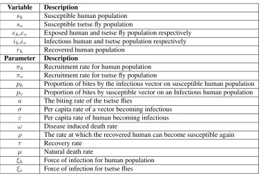
Table 1: The description of model variables and parameters

Variable Description

sh Susceptible human population

sv Susceptible tsetse fly population

eh,ev Exposed human and tsetse fly population respectively

ih,iv Infectious human and tsetse population respectively

rh Recovered human population

Parameter Description

πh Recruitment rate for human population

πv Recruitment rate for tsetse fly population

ph Proportion of bites by the infectious vector on susceptible human population

pv Proportion of bites by susceptible vector on an Infectious human population

a The biting rate of the tsetse flies

σ Per capita rate of a vector becoming infectious ε Per capita rate of human becoming infectious ω Disease induced death rate

ρ The rate at which the recovered human can become susceptible again τ Recovery rate

µ Natural death rate

ξh Force of infection for human population

ξv Force of infection for tsetse flies

The derivatives ofnh andnv with respect to time along the solution of system (2) for human and tsetse flies

respectively, are obtained by;

n0_h=dsh

dt + deh

dt + dih

dt + drh

dt ,

=πh−(sh+eh+ih+rh)µh−ωih,

=πh−nhµh−ωih.

n0_v =dsv

dt + dev

dt + div

dt,

=πv−(sv+ev+iv)µv,

=πv−nvµv.

From these differential equations it follows thatn0_h≤πh−µhnhandn

0

v ≤πv−µvnv. We obtain the solutions

as follows;

nh≤

πh

µh

(1−exp(−µht)) +nh(sh0, eh0, ih0, rh0) exp(−µht),

nv≤

πv

µv

(1−exp(−µvt)) +nv(sv0, ev0, iv0) exp(−µvt).

By taking the limits of bothnhandnvabove ast−→ ∞we obtainnh≤ π_µh

h andnv ≤

πv

µv, hence the solutions

given by;

D=

(sh, eh, ih, rh, sv, ev, iv)∈R7+:nh≤

πh

µh

;nv≤

πv

µv

.

3

Model Equilibria and Stability Analysis

In this section we give the model equilibria, the basic reproduction number,R0, and the stabilities at both disease

free and endemic equilibrium.

3.1

Disease-free Equilibrium(DFE)

The DFE in system (2) is when there are no HAT infections within the human and tsetse fly population. Thus the existence of the DFE is given by;E0=

_π

h

µh

,0,0,0,πv µv

,0,0

.

3.2

Endemic Equilibrium(EE)

The EE is the non-trivial equilibrium point at which the HAT disease persist in both human and tsetse fly popula-tion. Thus the EE is obtained as follows;E∗= (s∗h, e

∗

h, i

∗

h, r

∗

h, s

∗

v, e∗v, i∗v),where,

                                          

s∗_h = [πh(ρ+µh) +ρτ i

∗

h] [µv(σ+µv)(apvi∗h+µv)]

[a2_σp

hpvπvi∗h+µvµh(σ+µv)(apvi∗h+µv)] (µh+ρ)

,

e∗_h =(ω+τ+µh)i

∗

h

ε ,

r∗_h = τ i

∗

h

µh+ρ

,

s∗_v = πv

apvi∗_h+µv

,

e∗_v = apvπvi

∗

h

(σ+µv)(apvi∗_h+µv)

,

i∗_v = aσpvπvi

∗

h

(σ+µv)(apvi∗h+µv)µv

,

i∗_h =(ρ+µh)

a2εphpvπhπvσ−µ2vµh(ε+µh)(σ+µv)(µh+τ+ω)

B ,

(4)

the term

B= (apv(aσphπv(ερω+µh(ρ(τ+ω)+ε(ρ+τ+ω)+µh(ε+ρ+τ+ω+µh)))+µh(ε+µh)(ρ+µh)(τ+ω+µh)µv(σ+µv))).

3.3

Basic Reproduction Number,

R

The basic reproduction number,R0, is defined as the number of secondary infections caused by one infected host

or vector in a completely susceptible population [10]. Thenext generation matrixapproach as done byVan den DriesscheandWatmoughin [5, 11] is applied to derive

F= 

  

aphivsh

0

apvihsv

0



  

andV= 

  

µheh+εeh

−εeh+µhih+ωih+τ ih

µvev+δev

−δev+µviv



By denoting matrixF = ∂F

∂xi andV =

∂V

∂xi wherexi = eh, ih, ev, iv, the spectral radius of the next generation

matrixF V−1_{gives the value ofR} 0. F=            

0 0 0 aphsh

0 0 0 0

0 apvsv 0 0

0 0 0 0

           

andV =

           

ε+µh 0 0 0

−ε µh+ω+τ 0 0

0 0 µv+δ 0

0 0 −δ µv

            ,

F V−1=

              

0 0 aδph

µv(−δ+µv)

−aph

µv

0 apv

µh+τ+ω

0 0

0 0 0 0

0 0 0 0

               .

The spectral radiusσ(F V−1_)gives,

R0=σ(F V−1) =

s

a2_εp

hpvπhπvσ

µ2

vµh(ε+µh)(σ+µv)(µh+τ+ω)

.

One infected human in a population of susceptible vectors will cause Rv infected vectors, like wise, one

infected vector in a population will causeRhinfected humans [5]. Therefore the basic reproduction number can

be rewritten asR0=

√

RhRv, whereRh=

aεphπh

µh(µh+ε)(µh+τ+ω)

andRv =

σapvπv

µ2

v(σ+µv)

. Thus,R0can also

be defined as the square root of the product of the number of infected humans in the susceptible population caused by one infected tsetse fly in its infectious lifetime and the number of infected tsetse flies caused by one infected human during the infectious period [12].

3.4

Local Stability of Disease-Free Equilibrium(DFE)

Theorem 2. IfR0≤1the DFE given byE0is locally asymptotically stable in the region defined by Equation (3),

it is unstable whenR0>1.

Proof. The DFE is locally stable if all eigenvalues of Jacobian matrixJE0are negative. The matrix has all eigen-values negative only if the trace ofJE0 <0and determinant ofJE0 >0. By linearising system (2) aroundE0, we obtain the following Jacobian matrix;

JE0 =          

−µh 0 0 ρ 0 0 −aphsh

0 −(ε+µh) 0 0 0 0 aphsh

0 ε −(ω+τ+µh) 0 0 0 0

0 0 τ −(ρ+µh) 0 0 0

0 0 −apvsv 0 −µv 0 0

0 0 apvsv 0 0 −(σ+µv) 0

0 0 0 0 0 σ −µv

The trace of matrixJE0 is such that;

tr(JE0) =−(µh+ε+µh+µh+ω+τ+ρ+µh+µv+σ+µv+µv)

=−(4µh+ 3µv+ε+ω+τ+ρ+σ)<0.

Using the basic properties of matrix algebra as in [13], it is clear that the eigenvaluesλ1=−µhandλ2=−µvof

the matrixJE0have negative real parts. The reduced matrix is

JE1= 

    

−(ε+µh) 0 0 0 aphsh

ε −(ω+τ+µh) 0 0 0

0 τ −(ρ+µh) 0 0

0 apvsv 0 −(σ+µv) 0

0 0 0 σ −µv



     .

From matrixJE1 the eigenvalueλ3 =−(ρ+µh)has negative real part. The remaining matrix is further reduced by using the reduction techniques, we obtain;

JE2= 

         

−(ε+µh) 0 0 aphsh

0 −(ω+τ+µh) 0

aphshε

ε+µh

0 apvsv −(σ+µv) 0

0 0 σ −µv



          .

Using the properties of matrix algebra, the matrixJE2has eigenvalue−(ε+µh)which has negative real part. We further reduce to a2×2matrix by using the same reduction techniques. The matrix is

JE3= 

  

−(ω+τ+µh)

aphshε

ε+µh

apvsvσ

σ+µv

−µv



   .

From the reduced2×2matrix, the trace is negative and the determinant is,

Det(JE3) = (ω+τ+µh)µv− aphshε

ε+µh

×apvsvσ σ+µv

,

= (ω+τ+µh)µv

1− a

2_εp

hpvπhπvσ

µ2

vµh(ε+µh)(σ+µv)(µh+τ+ω)

.

Since

R0=

s

a2_εp

hpvπhπvσ

µ2

vµh(ε+µh)(σ+µv)(µh+τ+ω)

,

then, by lettingRT =

a2εphpvπhπvσ

µ2

vµh(ε+µh)(σ+µv)(µh+τ+ω)

, we find our determinant as,

Det(JE3) = (ω+τ+µh)µv[1−RT]. (5)

The value ofRT can be seen to be positive because all the parameters are positive. As a result, the determinant in

3.5

Global Stability of Disease-Free Equilibrium(DFE)

To show that the DFE is globally stable, we apply the Lypunov’s Theorem in [5].

Theorem 3. The DFE defined byE0 is globally asymptotically stable in the region defined by Equation (3) if

R0≤1. Otherwise unstable ifR0>1.

Proof. We define the Lypunov’s function as

V =k1

sh−sh0−sh0ln sh

sh0

+k2eh+k3ih+k4

sv−sv0−sv0ln sv

sv0

+k5ev+k6iv (6)

satisfying system (2), wherek1, k2, k3, k4, k5, k6>0are to be determined andsh0 = πh

µh

andsv0= πv

µv

. We first

show thatV >0for allE6=

_π

h

µh

,0,0,0,πv µv

,0,0

. It is enough to check that,

k1sh0

sh

sh0

−1−ln sh

sh0

>0,

k4sv0 _s

v

sv0

−1−ln sv

sv0

>0.

The functiong(m) =m−1−lnmsuch thatm= sh

sh₀ =

sv

sv₀ has minimum value equal to zero whenm= 1,

henceg(m) > 0for all m > 0. Thus the Lypunov’s function V > 0. The function V is radially unbounded because as|m|−→ ∞the functiong(m)−→ ∞. We now take the derivative ofV with respect to time and use system (2) to replace the derivatives in the right hand side such that;

V0 =k1

1−sh0 sh

_ds

h

dt +k2 deh

dt +k3 dih

dt +k4

1−sv0 sv

_ds

v

dt +k5 dev

dt +k6 div

dt,

=k1

1−sh0 sh

[πh+ρrh−aphivsh−µhsh] +k2[aphivsh−εeh−µheh]

+k3[εeh−µhih−ωih−τ ih] +k4

1−sv0 sv

[πv−µvsv−apvihsv]

+k5[apvihsv−µvev−σev] +k6[σev−µviv],

=2k1πh−aphshk1iv+ρrhk1−k1µhsh−k1

π2

h

µhsh

+aphπhiv

µh

k1−

πhρrh

µhsh

k1+k2aphshiv

−k2(ε+µh)eh+k3εeh−k3(τ+µh+ω)ih+ 2k4πv−k4apvsvih−µvsvk4−

πv2

µvsv

k4

+apvihπv

µv

k4−k5(µv+σ)ev+k5apvsvih+k6σev−k6µviv.

The terms withrhare ignored because ifsh, eh, ihare globally stable thenrh−→0at any timetand the DFE for

system(2)is globally stable. Takingk1=k2=_µ1

h+ε,k4=k5= 1

µv+σ,k3= 1

εandk6=

1

σ, the derivative ofV

V0=− πh µh+ε

_π

h

µhsh

+µhsh

πh

−2

−(τ+µh+ω) ε ih+

aphπh

(µh+ε)µh

iv−

πv

µv+σ

_π

v

µvsv

+µvsv

πv

−2

−µv σ iv+

apvπv

µv(µv+σ)

ih,

=−

_π

h

µh+ε

_π

h

µhsh

+µhsh

πh

−2

+ πv

µv+σ

_π

v

µvsv

+µvsv

πv

−2

+(τ+µh+ω)

ε

_εap

vπv

µv(σ+µv)(µh+τ+ω)

−1

ih+

µv

σ

_aσp

hπh

µvµh(µh+ε)

−1

iv,

=−

_π

h

µh+ε

_π

h

µhsh

+µhsh

πh

−2

+ πv

µv+σ

_π

v

µvsv

+µvsv

πv

−2

+(τ+µh+ω)

ε (Rv−1)ih+ µv

σ(Rh−1)iv.

The terms πh

µhsh +

µhsh

πh −2

and πv

µvsv +

µvsv

πv −2

are positive because if we supposem= πh

µhsh =

πv

µvsv,

we havem+_m1 −2 = m2−_m2m+1 = (m_m−1)2 >0for allm >1and sinceRv≤1andRh≤1thenV0is negative.

Thus we haveV0<0for allE06=

_π

h

µh

,0,0,0,πv µv

,0,0

.

Thus, the largest compact invariant set inDis the singleton setE0. Hence, system(2)is globally

asymptoti-cally stable.

3.6

Local Stability of Endemic Equilibrium(EE)

Theorem 4. The unique endemic equilibrium defined byE∗is locally asymptotically stable in the region defined by Equation (3) ifR0>1, but is unstable ifR0≤1.

Proof. We give the proof of this theorem based on the approach used by [9, 14]. From theEEpoints defined in Equation(4), since all values are positive, we express the value ofi∗_hin terms ofR0to obtain;

i∗_h= µ

2

vµh(ε+µh)(ρ+µh)(σ+µv)(µh+τ+ω)

B

_a2_εp

hpvπhπvσ

µ2

vµh(ε+µh)(σ+µv)(µh+τ+ω)

−1

,

= µ

2

vµh(ε+µh)(ρ+µh)(σ+µv)(µh+τ+ω)

B

R20−1

,

where

B= (apv(aσphπv(ερω+µh(ρ(τ+ω)+ε(ρ+τ+ω)+µh(ε+ρ+τ+ω+µh)))+µh(ε+µh)(ρ+µh)(τ+ω+µh)µv(σ+µv))).

Since the basic reproduction number,R0=

s

a2_εp

hpvπhπvσ

µ2

vµh(ε+µh)(σ+µv)(µh+τ+ω)

, if we let

RT =

a2εphpvπhπvσ

µ2

vµh(ε+µh)(σ+µv)(µh+τ+ω)

,

then we can findi∗_has,

i∗_h= µ

2

vµh(ε+µh)(ρ+µh)(σ+µv)(µh+τ+ω)

The value ofB is clearly positive because all parameters are positive. Hence, i∗_h > 0if and only ifRT > 1,

implying that theEEis locally asymptotically stable ifRT >1.

3.7

Global Stability of Endemic Equilibrium(EE)

To show the global stability of theEEwe use Lyapunov’s Theorem together with the following Lemma.

Lemma 1. Suppose thaty1, y2,· · ·, ynarenpositive numbers, then their arithmetic mean is greater than or equal

to the geometric mean, that’sy1+y2+· · ·+yn

n ≥(y1y2· · ·yn) 1 n.

Theorem 5. The EE defined byE∗is globally asymptotically stable ifR0>1, otherwise is unstable.

Proof. The proof is based on the idea as explained by [5]. We define the Lyapunov function as

V =k1

sh−s∗h−s∗hln

sh

s∗_h

+k2

eh−e∗h−e∗hln

eh

e∗_h

+k3

ih−i∗h−i∗hln

ih

i∗_h

+k4

sv−s∗v−s∗vln

sv

s∗

v

+k5

ev−e∗v−e∗vln

ev

e∗

v

+k6

iv−i∗v−i∗vln

iv

i∗

v

satisfying system (2) with k1, k2, k3, k4, k5, k6 > 0 to be determined. The function V is non negative for all

(sh, eh, ih, rh, sv, ev, iv)6= (sh∗, e∗h, i∗h, rh∗, s∗v, e∗v, i∗v)and radially unbounded.

We need to prove that V0 < 0 for all (sh, eh, ih, rh, sv, ev, iv) = (6 s∗h, e∗h, i∗h, rh∗, s∗v, e∗v, i∗v). We find the

derivative ofV with respect to time and replace the derivativess0_h, e0_h, i0_h, r0_h, s0_v, e0_v, i0_vwith system (2). We also ignore therhterms because ifsh, eh, ihare globally stable thenrh−→0at any timetandEEis globally stable.

V0 =k1

1−s

∗

h

sh

[πh−aphivsh−µhsh] +k2

1−e

∗

h

eh

[aphivsh−(µh+ε)eh]

+k3

1−i

∗

h

ih

[εeh−(ω+τ+uh)ih] +k4

1−s

∗

v

sv

[πv−apvihsv−µvsv]

+k5

1−e

∗

v

ev

[apvihsv−(µv+σ)ev] +k6

1−i

∗

v

iv

[σev−uviv].

We now substituteπh=aphi∗vs∗h+µhs∗handπv=apvi∗hs∗v+µvs∗vat the endemic equilibrium then simplify and

put similar terms together to obtain;

V0 =−k1

(sh−s∗h)

2

µh

sh

+k1aphi∗vs∗h−k1aphivsh−k1aph

s∗_h2i∗_v sh

+k1aphivs∗h+k2aphshiv−k2(ε+µh)eh

−k2aphshiv

e∗_h eh

+k2(ε+µh)e∗h+k3εeh−k3(ω+τ+µh)i∗h−k3εeh

i∗_h ih

+k3(ω+τ+µh)i∗h

−k4

(sv−s∗v)

2

µv

sv

+k4apvi∗hs∗v−k4apvihsv−k4apv

s∗_v2i∗_h sv

+k4apvihs∗v+k5apvsvih−k5(σ+µv)ev

−k5apvsvih

e∗_v ev

+k5(σ+µv)e∗v+k6σev−k6µvi∗v−k6σev

i∗_v iv

We supposek1=k2andk4=k5, and multiply and divide the same equilibrium value to some of the fractions to

obtain;

V0=−k1

(sh−s∗h)

2

µh

sh

+k1aphi∗vs

∗

h−k1aph

s∗_h2i∗_v sh

+k1aphivs∗h−k2(ε+µh)eh

−k2aphshiv

e∗_hs∗_hi∗_v s∗

hi∗veh

+k2(ε+µh)e∗h+k3εeh−k3(ω+τ+µh)ih−k3εeh

i∗_he∗_h ihe∗h

+k3(ω+τ+µh)i∗h

−k4

(sv−s∗v)

2

µv

sv

+k4apvi∗hs

∗

v−k4apv

s∗_v2i∗_h sv

+k4apvihs∗v−k5(σ+µv)ev

−k5apvsvih

e∗_vs∗_vi∗_h s∗

vi∗hev

+k5(σ+µv)e∗v+k6σev−k6µvi∗v−k6σev

e∗_vi∗_v ive∗v

+k6µvi∗v.

We choose k3 = k2µh_ε+ε such that k3(ω +τ+µh)ih∗ = k2(ε+µh)eh∗ and choosek6 = k5µh_σ+σ such that

k6µvi∗v =k5(σ+µv)e∗v. Nowaphs∗hi∗v= (µh+ε)e∗handapvs∗vi∗v = (µv+σ)e∗vbecausek1=k2andk4=k5

respectively. We now obtain;

V0 =−k1

(sh−s∗h)

2

µh

sh

+k1aphi∗vs

∗

h

3−s

∗

h

sh

−e

∗

hivsh

s∗

hehi∗v

−ehi

∗

h

ihe∗h

+k1aphivs∗h−k3(ω+τ+µh)ih

+ [k3ε−k2(ε+µh)]eh−k4

(sv−s∗v)

2

µv

sv

+k4apvi∗hs

∗

v

3−s

∗

v

sv

−e

∗

vihsv

s∗

vevi∗h

−evi

∗

v

ive∗v

+k4apvihs∗v−k6µviv+ [k6σ−k5(σ+µv)]ev.

Supposek6=k1aphs ∗ h

µv andk3=

k4apvs∗v

ω+τ+µh, we then substitute and simplify to get

V0=−k1

(sh−s∗h)

2

µh

sh

+k1aphi∗vs

∗

h

3−s

∗

h

sh

−e

∗

hivsh

s∗_hehi∗v

−ehi

∗

h

ihe∗_h

−k4

(sv−s∗v)

2

µv

sv

+k4apvi∗hs∗v

3−s

∗

v

sv

−e

∗

vihsv

s∗

vevi∗h

−evi

∗

v

ive∗v

.

From Lemma1above, the terms

k1aphi∗vs∗h

h

3−s∗h

sh −

e∗_hivsh

s∗ hehi∗v −

ehi∗h

ihe∗h i

andk4apvi∗hs∗v

h

3−s∗v

sv −

e∗_vihsv

s∗ vevi∗h

−evi∗v

ive∗v i

≤0.

Therefore,V0<0for all(sh, eh, ih, rh, sv, ev, iv)= (6 s∗h, e∗h, i∗h, rh∗, s∗v, e∗v, i∗v)implying that the endemic

equilib-rium is globally asymptotically stable ifR0>1.

4

Analysis of Optimal Control Model

In this section, we formulate the optimal control model by modifying system (2) to an optimal control problem. We thus define some linear functionsci(t) = 1, fori = 1,2,3. It is important to note that controls are fully

effective whenci(t) = 1and not effective whenci(t) = 0. The forces of infectionξhandxivwhich correspond to

the human and vector population respectively, are reduced by the factor(1−c1); wherec1measures the level of

success obtained due to the effort of educating people on the dangers of exposing their skin, and encouraging them to wear long sleeves and long pants during the day to minimize tsetsefly-human contacts. The factorc2represents

the effort of treatment to control the disease and the factorc3also represent the effort of using insecticides to ensure

made, we try to find the most effective strategy that reduces the HAT infection in the population at a very minimum cost. With the use of bounded Lebesgue measurable control, we define the objective function to be minimized as

J(c1, c2, c3) =

Z tF

0

M1eh+M2ih+M3ev+M4iv+

1 2k1c

2 1+

1 2k2c

2 2+

1 2k3c

2 3

dt. (7)

Thus, the dynamics of the controls that minimizes the objective function is given by                        dsh

dt =πh+ρrh−(1−c1)aphivsh−µhsh deh

dt = (1−c1)aphivsh−εeh−µheh dih

dt =εeh−µhih−ωih−c2τ ih drh

dt =c2τ ih−ρrh−µhrh dsv

dt =πv−c3µvsv−(1−c1)apvihsv dev

dt = (1−c1)apvihsv−c3µvev−σev div

dt =σev−c3µviv,

(8)

subject to the initial conditionssh ≥0, eh ≥0, ih ≥0, rh ≥0, sv ≥0, ev ≥0, iv ≥0. The associated effective

reproduction number for Equation(8)denoted byREis obtained as

RE=

s

a2_ε(1−c

1)2phπhπvσ

c3µh(ε+µh)µ2v(σ+c3µv)(µh+c2τ+ω)

=pRc. (9)

The goal is to minimize the exposed and infectious human populations(eh, ih), the exposed and infectious vector

populations(ev, iv)and the cost of implementing the control by the use of possibleci, i= 1,2,3. The functional

objective includes the social cost which relates to the resources that is needed for educating people on personal protection 1₂k1c21, the application of treatment

1 2k2c

2

2and spraying of tsetsefly operations 1 2k3c

2

3. The quantities

M1 andM2 respectively represent the associated cost with minimizing the exposed and infected human

pop-ulation, whileM3 andM4 also represent the cost associated with minimizing the exposed and infected vector

respectively. The quantitytF is the time period of intervention. As explained in [17], the costs corresponding

toM1eh, M2ih, M3evandM4iv are linear while the cost control functions 1₂k1c21, 1 2k2c

2 2,and

1 2k3c

2

3should be

nonlinear and take a quadratic form. Therefore, we seek to minimize the objective function over the given time interval[0, tF]. Pontryagin’s Maximum Principle is used to solve this optimal control problem and the derivation

of the necessary conditions. The Lagrangian of the optimal control problem is given by

L=

M1eh+M2ih+M3ev+M4iv+

1 2k1c

2 1+

1 2k2c

2 2+

1 2k3c

2 3

. (10)

To determine the Lagrangian minimum value, we define the Hamiltonian,H, for the control problem as

H =M1eh+M2ih+M3ev+M4iv+

1 2k1c

2 1+

1 2k2c

2 2+

1 2k3c

2 3+λsh

dsh

dt +λeh

deh

dt +λih

dih

dt

+λrh

drh

dt +λsv

dsv

dt +λev

dev

dt +λiv

div

dt,

whereλsh, λeh, λih, λrh, λsv, λev, λiv are adjoint variables or co-state variables. The differential equations of

            

           

dλ_sh

dt =λshµh+ (λsh−λeh)(1−c1)aphiv

dλ_eh

dt =−M1+ (λeh−λih)ε+λehµh

dλ_ih

dt =−M2+ (λih−λrh)c2τ+λih(ω+µh) + (λsv −λev)(1−c1)apvsv

dλ_rh

dt = (λrh−λsh)ρ+λrhµh

dλ_sv

dt = (λsv−λev)(1−c1)apvih+λsvµvc3

dλev

dt =−M3+ (λev−λiv)σ+λevµvc3

dλ_iv

dt =−M4+ (λsh−λeh)(1−c1)aphsh+λivµvc3.

(11)

Theorem 6. Given the optimal controlsc∗₁, c∗₂, c∗₃ and the solutionssh, eh, ih, rh, sv, ev, iv of the corresponding

state Equations (8) and (7) which minimizeJ(c1, c2, c3)over the region Ω, then there exist adjoint variables

λsh, λeh, λih, λrh, λsv, λev, λiv satisfying

−dλi dt =

∂H

∂i i∈ {sh, eh, ih, rh, sv, ev, iv},

and the optimal solutionc∗₁, c∗₂, c∗₃is given by

c∗₁= min{1,max(0,c_b1)},

c∗2= min{1,max(0,cb2)},

c∗₃= min{1,max(0,c_b3)}.

Proof. The Pontryagin’s Maximum principle described in [15, 16] is applied. The Corollary4.1 in [16] shows the existence of an optimal control due to the convexity of the integrandJ with respect toc1, c2, c3, and Lipschitz

property of the state system with respect to the state variables. By using the optimal conditions, ∂H

∂c1

= 0, ∂H ∂c2

= 0, ∂H ∂c3

= 0,

we obtain,

  

 

∂H

∂c1 =k1c1+ (λsh−λeh)aphivsh+ (λsv −λev)apvihsv = 0,

∂H

∂c2 =k2c2+ (λrh−λih)τ ih= 0,

∂H

∂c3 =k3c3−(λsvµvsv+λevµvev+λivµviv) = 0.

(12)

Solving Equation (12) we have,

b c1=

(λeh−λsh)aphivsh+ (λev−λsv)apvihsv

k1

,

b c2=

(λih−λrh)τ ih

k2

,

b c3=

λsvµvsv+λevµvev+λivµviv

k3

.

As stated earlier, the lower and upper boundaries for the control parameters are 0 and 1 respectively. If

b

c1,cb2,cb3<1thenc1=c2=c3= 0and ifcb1,cb2,cb3>1thenc1=c2=c3= 1otherwisec1=cb1, c2=cb2, c3=

b

4.1

Optimal Control Simulations

The Octave programming language is used to simulate the optimal control model using the set of parameters obtained from previously reported studies and datasets, which have been cited. Some of these parameters are assumed for the sake of illustrations. Table2represents the values of the model parameters used for simulations. The following initial conditions were considered,

sh(0) = 30, eh(0) = 7, ih(0) = 2, rh(0) = 0, sv(0) = 40, ev(0) = 10, iv(0) = 3,

and the weight constants were assumed to be

M1= 1, M2= 2, M3= 2, M4= 2, k1= 2, k2= 10, k3= 5.

Table 2: Parameters values used for simulations

Parameter Value Reference

πh 0.000215/day [14]

πv 0.07/day [14]

ph 0.62 [6]

pv 0.065 [6], [17]

a varying Assumed

σ 0.001 Assumed

ε 0.083 [18]

ω 0.004 [3]

ρ 0.02 [6]

τ 0.125 [3]

µh 0.00044 Assumed

µv 0.034 [17]

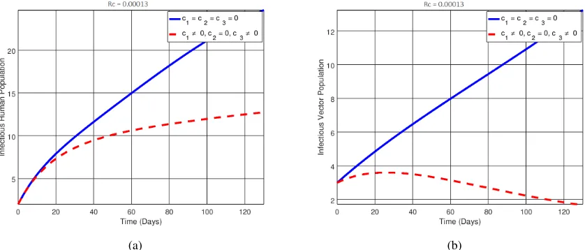
The Figures2 and3 represent the control profiles at different values ofc1, c2 andc3 while the rest of the

plots are the graphs of infectious human and vector population plotted against time in days and they represent the effect of optimal controlsc1, c2andc3in reducing the number of individuals infected. From Figure4we observe

(a) (b)

Figure 2: (a) Control Profile whenc1= 0,c26= 0andc36= 0. (b) Control profile whenc16= 0, c2= 0andc36= 0.

(a) (b)

Figure 3: (a) Control Profiles whenc1 6= 0, c2 6= 0andc3 = 0. (b) Control profile whenc1 6= 0, c2 6= 0,and

c36= 0.

(a) (b)

(a) (b)

Figure 4: Simulations of the model showing the efforts of treatment and insecticides only on infectious individuals.

(a) (b)

Figure 6: Simulations of the model showing the efforts of education and treatment only on infectious individuals.

(a) (b)

In epidemiology, a reproduction number less than unity implies that the disease can be eradicated in the long run. Hence, choosing suitable parameters for the controlsc1, c2 andc3, it was observed that the effective

repro-duction number obtained for Figures2(a),2(b),3(a),3(b),4,5,6, and7were0.0075,0.00013,0.044,0.000075,

0.0075,0.00013,0.044and0.000075respectively. This shows that by incorporating all the control measures that is educating individuals, giving treatment and applying insecticides is an effective method to help reduce the number secondary infections in the population which corresponds with eradicating the disease in the long run.

5

Conclusion

In this paper, we studied and analysed the model for transmission of HAT, and determined the basic reproduction number. The local and global stabilities of disease free equilibrium and endemic equilibrium were also proved. For the optimal control model, education, treatment and insecticides as control measures were used to optimize the objective function defined by Equation (7). The numerical simulations of the optimal control model shows that the best strategy to reduce the number of infected individuals is through the use of both education, treatment and insecticides. This is the effective and efficient method to eliminate the disease. Furthermore, the national authorities, Non-Governmental Organizations (NGOs), and stakeholders must not lose their interest in controlling the disease because neglecting this disease may cause the rapid re-occurrence and much effect to the people who are at risk.

6

Conflicts of Interest

The authors declare that they have no conflicts of interest.

7

Acknowledgements

The first author’s work (thesis) was partly supported by the Next Einstein Initiative of the African Institute for Mathematical Sciences, Ghana, Annual Grant for Graduate Studies.

8

Data Availability Statement

References

[1] Rock, K.S., Torr, S.J., Lumbala, C., Keeling, M.J.: Quantitative evaluation of the strategy to eliminate human african trypanosomiasis in the democratic republic of congo. Parasites & vectors8(1), 532 (2015)

[2] Franco, J.R., Simarro, P.P., Diarra, A., Jannin, J.G.: Epidemiology of human african trypanosomiasis. Clinical epidemiology6, 257 (2014)

[3] Brun, R., Blum, J., Chappuis, F., Burri, C.: Human african trypanosomiasis. The Lancet375(9709), 148–159 (2010)

[4] Organization, W.H.,et al.: Control and Surveillance of Human African Trypanosomiasis: Report of a WHO Expert Committee. World Health Organization, ??? (2013)

[5] Martcheva, M.: An Introduction to Mathematical Epidemiology vol. 61. Springer, ??? (2015)

[6] Rogers, D.J.: A general model for the african trypanosomiases. Parasitology97(1), 193–212 (1988)

[7] Hargrove, J.W., Ouifki, R., Kajunguri, D., Vale, G.A., Torr, S.J.: Modeling the control of trypanosomiasis using trypanocides or insecticide-treated livestock. PLoS neglected tropical diseases6(5), 1615 (2012)

[8] Kajunguri, D.: Modelling the control of tsetse and african trypanosomiasis through application of insecticides on cattle in southeastern uganda. PhD thesis, Stellenbosch: Stellenbosch University (2013)

[9] Olaniyi, S., Obabiyi, O.S.: Mathematical model for malaria transmission dynamics in human and mosquito populations with nonlinear forces of infection. International Journal of Pure and Applied Mathematics88(1), 125–156 (2013)

[10] Chisholm, R.H., Campbell, P.T., Wu, Y., Tong, S.Y.C., McVernon, J., Geard, N.: Implications of asymp-tomatic carriers for infectious disease transmission and control. Open Science5(2), 172341 (2018)

[11] Yan, P., Liu, S.: Seir epidemic model with delay. The ANZIAM Journal48(1), 119–134 (2006)

[12] Azu-Tungmah, G.T.: A mathematical model to control the spread of malaria in ghana. PhD thesis (2012)

[13] Pedro, S.A., Abelman, S., Ndjomatchoua, F.T., Sang, R., Tonnang, H.E.Z.: Stability, bifurcation and chaos analysis of vector-borne disease model with application to rift valley fever. PloS one9(10), 108172 (2014)

[14] Olaniyi, S., Obabiyi, O.S.: Qualitative analysis of malaria dynamics with nonlinear incidence function. Ap-plied Mathematical Sciences8(78), 3889–3904 (2014)

[16] Heimann, B.: Fleming, wh/rishel, rw, deterministic and stochastic optimal control. new york-heidelberg-berlin. springer-verlag. 1975. xiii, 222 s, dm 60, 60. ZAMM-Journal of Applied Mathematics and Mechan-ics/Zeitschrift für Angewandte Mathematik und Mechanik59(9), 494–494 (1979)

[17] Davis, S., Aksoy, S., Galvani, A.: A global sensitivity analysis for african sleeping sickness. Parasitology

138(4), 516–526 (2011)