Climate targets and cost-effective climate stabilization
pathways
H. Held(∗)(∗∗)
Research Unit Sustainability & Global Change, Departments of Geosciences and Economics, University of Hamburg - KlimaCampus, Grindelberg 5, 20144 Hamburg, Germany
Summary.— Climate economics has developed two main tools to derive an
eco-nomically adequate response to the climate problem. Cost benefit analysis weighs in any available information on mitigation costs and benefits and thereby derives an “optimal” global mean temperature. Quite the contrary, cost effectiveness anal-ysis allows deriving costs of potential policy targets and the corresponding cost-minimizing investment paths. The article highlights pros and cons of both ap-proaches and then focusses on the implications of a policy that strives at limiting global warming to 2◦C compared to pre-industrial values. The related mitigation costs and changes in the energy sector are summarized according to the IPCC report of 2014. The article then points to conceptual difficulties when internalizing uncer-tainty in these types of analyses and suggests pragmatic solutions. Key statements on mitigation economics remain valid under uncertainty when being given the ade-quate interpretation. Furthermore, the expected economic value of perfect climate information is found to be on the order of hundreds of billions of Euro per year if a 2◦-policy were requested. Finally, the prospects of climate policy are sketched.
(∗) Also guest at the Potsdam Institute for Climate Impact Research e.V. (PIK), Telegrafenberg, 14412 Potsdam, Germany.
(∗∗) E-mail:[email protected]
/ /
7KLVLVDQ2SHQ$FFHVVDUWLFOHGLVWULEXWHGXQGHUWKHWHUPVRIWKH&UHDWLYH&RPPRQV$WWULEXWLRQ/LFHQVHZKLFKSHUPLWV C
1. – The rationale of climate targets
The following article strives at linking the debates on possible paths of energy system transitions and mitigating global warming. It follows two presentations given at the Joint EPS-SIF International School on Energy 2014, Varenna. It constitutes a second edition of the article that emerged from the precursory summer school in 2012 [1], hereby with stronger emphasis on findings of the IPCC (Intergovernmental Panel on Climate Change), as from 2013 to 2014 the IPCC released its latest and fifth report.
The IPCC’s goal is to summarize the present status of research on the causal link between greenhouse gas emissions and global warming, on impacts of global warming and on adaptation or mitigation measures. It is a unique instance in the history of science(1) that a whole research field organizes a process which every 5-7 years culminates in the release of a report stating not only the degree of academic consensus, but also dissent among scientists on a certain matter. This in turn represents a unique service to society who thereby gets access to the state of knowledge of an interdisciplinary research field in a balanced way and within relatively short time frame — as compared to the “trickle-down time” it usually takes for the dissemination of fundamentally new academic insights.
One of the key statements in the above-mentioned IPCC report reads: “Anthro-pogenic greenhouse gas emissions have increased since the pre-industrial era, driven largely by economic and population growth, and are now higher than ever. This has led to atmospheric concentrations of carbon dioxide, methane and nitrous oxide that are unprecedented in at least the last 800000 years. Their effects, together with those of other anthropogenic drivers, have been detected throughout the climate system and are extremely likely to have been the dominant cause of the observed warming since the mid-20th century.” [2]. For the remainder of this article, I assume the causal link from greenhouse gas emissions and the increase of global mean temperature as given in order to concentrate on the question how the global society could rationally respond to global warming. Nevertheless in the Section “Investment under Uncertainty” I explicitly acknowledge that the magnitude of global warming induced by carbon dioxide emissions is subject to uncertainty that is on the same order of magnitude as the warming effect as such(2).
Given the phenomenon of anthropogenically caused global warming one may now ask: Should society take action in mitigating part of the anticipated future global warming? There are two traditions of thought that come with subsequent tools of analysis within climate economics to tackle this question. The first rests on “positive knowledge”, i.e. the explicitly known consequences of global warming. The second working group of
(1) I hereby use “science” in the generalized sense that includes any academic endeavor that comprises a cycle of observation, hypothesizing, theory building, theory/model-observational data intercomparison and thereby further stimulated observation. In particular, this comprises the natural sciences but also,e.g., those parts of economics or social science that would subscribe to this cyclic paradigm.
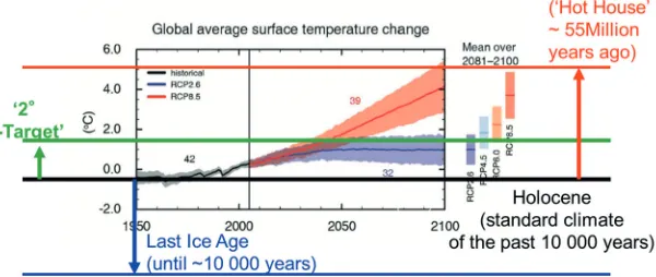
Fig. 1. – Operationalizing the precautionary principle for the global mean temperature (GMT) rise. The 2◦target (which should more correctly be called “2◦limit”) is closer to the Holocene (black line) rather than to the Holocene temperature elevated by the “natural GMT scale”,
i.e.the difference between Holocene GMT and last ice age GMT (red line). That GMT was realized during the Eocene 55 million years ago [4]. Note that the latter is in fact in reach for this century for the high end of emission scenarios.
the IPCC [3] is mainly devoted to impacts of global warming that comprise inter alia changes in extreme weather event statistics, loss of ecosystems, or sea level rise. After having introduced key elements of economic reasoning below, I will briefly summarize some findings along this school of thought.
A second stream of argument rests on the notion that human action might drive the system into modes of operation the consequences of which would be hard to predict. This is an instance where some actors would find that the precautionary principle should be applied. (In fact, the EU commission has officially subscribed to the precautionary principle [5].) The latter would state that as the uncertainty coming with the outcome of an action is currently too large, we should avoid that action. The question then is: how would one operationalize the precautionary principle in the case of global warming? For major parts of the discussion, the academic construct of the “global mean temperature” (GMT) serves as an indicator for the “state of the climate system”. This has scientific backing, as GMT change strongly correlates with impacts. On the other hand it serves as a politically useful simplification of the discussion when it comes to negotiating targets. So if we accept that GMT is a useful quantity to discuss climate policy, we would then ask: What could be a natural scale that would allow us to calibrate what is a “small” or a “large” deviation from the “natural state”? One scale that suggests itself is the GMT difference between the last ice age and the current pre-industrial “standard climate”, the Holocene that has prevailed for the last 10000 years. This temperature difference is 5 K [6]. One way to operationalize the precautionary principle would then be to request that GMT should be closer to the Holocene GMT than to a Holocene GMT elevated by 5 K (see fig. 1).
supported by the German Advisory Council on Global Change (WBGU), then by the EU and finally on the global level by the Conference of the Parties [8]. There are three lines of argument that support the target. Firstly, it can be interpreted as a realization of the precautionary principle along the lines as indicated above.
Secondly, the 2◦target does also recognize positive knowledge about climate damages, in particular about extreme event statistics “It is very likely that heat waves will occur more often and last longer, and that extreme precipitation events will become more intense and frequent in many regions” [2].
Thirdly, the 2◦ target is a political target in that it massively reduces complexity of the debate by channeling it into a single number. In that sense it also acts in analogy to a speed limit on motorways, without claiming any sort of phase transition in the natural system, when the 2◦ limit would have been transgressed. The latter point is extremely important to note in case it might have become clear one day that it will be impossible to observe the target any longer, after mitigation has been postponed for further decades. If it indicated a phase transition, this might support the notion that then it would not matter any longer how much mitigation we still would implement — it was “too late” anyhow and then we would switch back to a no-mitigation policy case. However, if the 2◦-target was merely a semi-political target, still as much mitigation as possible might be regarded as desirable even if the limit was transgressed.
What would a 2◦target imply in terms of necessary emission savings? During the past years climate scientists could identify the so-called “emission budget” or “carbon budget”, the time-integral of global carbon dioxide emissions until 2050 or 2100 as an approximate predictor of maximum temperature if emissions more or less vanish thereafter. The physical reason lies in the fact that due to its heat capacity the global ocean acts as a low-pass filter with a time-scale of approximately 50 years (if one wanted to approximate global mean temperature response to carbon dioxide emissions) and a similar filtering scale in the carbon cycle. Accordingly 1000 GtCO2(3) could be emitted 2000–2049 [9] to be in compliance with the 2◦target with a probability of 2/3. The concept of the carbon budget will be needed below.
2. – Cost benefit versus cost effectiveness analysis
These two schools of thought have their counterparts within the economic community. Within environmental economics, the standard tool is cost benefit analysis (CBA). Costs of an environmental intervention (in our case: implementing a mitigation policy) are to be traded off against avoided (environmental) damages (in our case: damages minus some benefits from global warming). The archetypical analysis of this kind was undertaken by [10]. By definition the analysis involves positive knowledge on global warming impacts. Generically, results of this kind of analysis would recommend emission trajectories that would be at odds with complying with the 2◦target (see,e.g., [11]) — in the sense that
they would regard higher emissions as “economically optimal”. This reveals that either both camps have opposing normative views or make use of different data sources.
CBAs of this kind have been criticized for various reasons (e.g.[12]). The arguments can be divided into the following three classes: i) Today it is rather impossible to draw on an approximate library of impacts of global warming on the natural system, ii) For a significant fraction of these impacts no markets exist, hence non-market–based eval-uation methods would have to be applied. For most of such impacts, however, societal discussions rather than economic extrapolations would be in order, which have not yet been realized. iii) CBA of the climate problem necessarily involves trading off costs of transforming the energy system over the next decades with avoided damages that would occur over the next 50–1000 years(4). But how to trade off the present against the future is presently an unsettled conceptual issue within climate economics:
(1) Max!W :=
∞
t0
U(t)e−r(t−t0)dt.
The latter appears conceptually especially salient, as standard macro-economic tools involve optimizing the linear time-average of exponential discounted utility (“utility” can be interpreted as the material basis for “happiness”). There is an ongoing debate on whether the discounting parameterrwas a descriptive or normative parameter, the key arguments of which are already summarized in [13]. If it was to be interpreted as a descriptive parameter, it should be linked to the current interest rate. Accordingly some would then discount the future to the extent that the utility of the grandchildren’s generation would be worth in the order of percent of that of the present generation. That is why others would setr almost to zero [14] arguing that when applying eq. (1) to the climate problem, it represents a normative approach to shaping the future andr is to be politically negotiated accordingly. “Hyperbolic discounting” would allow combining a short-term high with a long-term decaying discount rate which seems to serve the value system of environmentalists. However one can show that only exponential discounting does deliver recommendations that are “time-consistent”(5), an in my view indispensable property of any normative theory. Finally, in a recent development, others argue that the whole model represented by eq. (1) was too narrow and the normativeversus descriptive trade-off ill-posed [15]. However the latter implies deviating from linear intertemporal averages, hence are hard to interpret and require further investigations.
All of these conceptual challenges have led a fraction of climate economists to the con-viction that for the time being a less ambitious approach is necessary (for some overview on this type of discussion see,e.g., [12, 16], or [17]). Cost effectiveness analysis (CEA)
(4) Due to the twin-integrating effect from emissions to concentrations to warming the upper ocean, in combination with the existing pools of carbon and the heat capacity of the ocean, the climate system would likely respond to a climate policy only within the next 50 years.
(or, more precisely, “constrained welfare-optimization”) just asks for the economic loss of a certain environmental target without attempting to trade off that loss against future benefits, and hence without judging to what extent that target would be economically optimal in any sense. As in business-as-usual scenarios of climate change the energy sec-tor would be responsible for most of the reasons for future global warming, a CEA of the 2◦ target simply addresses the question: What are the costs of transforming the energy system in line with the 2◦ target? In case the costs turn out to be “low”, society could take action from a macro-economic point of view: environmentalists could be satisfied because at least a minimum environmental standard would be implemented. Economists supportive of CBA might argue that the target was not economically optimal, but they could acknowledge that at least the economic loss was “acceptable”. In that sense, the 2◦ target would act as an “insurance premium” to avoid uncertainty.
Thereby, CEA elegantly bypasses one currently unsolvable problem of CBA for the next years of decision-making: it does not need to express the totality of global warming impacts economically (because CEA does not account for damages at all). Moreover one could even argue that it also moderates a strong dependence of a welfare optimal policy on the pure rate of time preference r. In principle CEA suffers from the same formal dependence as CBA does, as also CEA utilizes to maximize welfare. However, it does so under the constraint that 2◦ shall not be transgressed. Numerically it will turn out that this implies that a transformation of the global energy system towards low-emission technologies would have to be carried out over the next decades (see,e.g., [18])— thus, welfare changes are considered basically now and not in a hundred years as in CBA. As a result,rdoes numerically not matter as much for CEA as it would for CBA.
Consequently, the key question is: Are the costs of the 2◦ target in fact so “small” that a consensus on mitigation action could emerge within society? Integrated assessment modeling tries to address this question as outlined below:
3. – Integrated assessment models for CEA of the climate problem
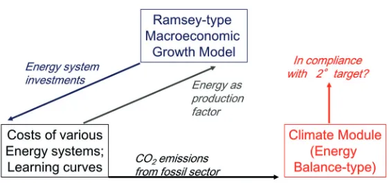
Models that represent sectors as remote in the academic system as economy, en-ergy and climate and dynamically link them are called “Integrated Assessment Models” (IAMs). In our case the three mentioned sectors are represented by individual modules. Figure 2 depicts the coupling scheme of the economic, the energy and the climate module in an IAM of CEA of the climate problem for an assumed 2◦target. Such a scheme would deliver the optimal investment time series, optimal in the sense that welfare would be optimized under the constraint that society complied with the 2◦ target. Without that constraint we would get a “business as usual” (BAU) case that describes a fictitious world without a mitigation policy and without any climate damages. The welfare difference between the two scenarios can be re-interpreted as “mitigation costs” — the costs to transform the energy system. Note that saved damages are not part of that equation, hence the net costs of the 2◦ target are smaller or even negative.
com-Fig. 2. – Scheme of integrated assessment models that execute a cost effectiveness analysis of temperature targets, such as the 2◦ target. In the model, an economic kernel would supply investments to various energy technologies and receives energy as an input for macro-economic production. Depending on the energy technology used, greenhouse gases will be produced that are handed over to the climate module. The latter would test whether the emission time series is compatible with the 2◦ target. If it violates the target, fewer investments into emitting technologies would be undertaken. In the end, investment time series are derived that optimize the economic welfare under the constraint that 2◦warming is not transgressed.
pliance with the 2◦target. When prescribing a concentration target one can save part the second half of the influence chain from emissions to concentration change to temperature change in the climate module and hence some computational effort. However thereby one complies with the temperature limit only in approximate terms or one reaches the welfare optimum only approximately, or both. To my impression, a CEA based on a well-chosen concentration target can lead to a good approximation of a CEA based on a temperature target. However, to the best of my knowledge, no systematic investigation of the welfare loss induced by imposing an auxiliary concentration target has been performed yet.
Max!W :=
∞
t0
U(t)e−r(t−t0)dt, (2)
subject to∀tT(t)< T∗.
In the following I describe pars pro toto the structure of the MIND model and its derivative, the ReMIND model, as they represent leading IAMs for a centennial time horizon for inter related energy-climate research questions. That model suite has signif-icantly contributed to the Stern report in 2007 as well as the IPCC report of 2014.
planner(6) anticipates to produce more in the future and, accordingly, also plans to be in a position to consume more in the future if not all of today’s production is consumed. The control variable’s time series is made up by the time series of investment into various energy technologies. (Economists have a somewhat different lingo than physicists here: for them, a “time series” is a “path”, hence they speak of a “control path”.) “Utility” is a monotonously increasing, concave function of consumption. Through the climate module a temperature constraint is superimposed (see eq. (2)). Thereby the optimization problem is defined.
The energy system module must resolve problems in connection with presently rela-tively cheap fossil fuels in the near future and, even earlier, more expensive low-carbon energy technologies. The ReMIND model resolves on the order of one hundred energy technologies. Technologies are assumed to have some potential for cost reduction. In fact so-called “learning curves” (more precisely “experience curves”) have been observed for most products, including energy technologies. The costs per unit of energy deliv-ered in terms of electricity have fallen by orders of magnitude for photovoltaic and wind power [19]. Academia knows two extreme models to explain this phenomenon: “exoge-nous” and “endoge“exoge-nous” technological change.
The former hypothesis states that there is overall learning in the globalized market across all sectors and hence, also a particular energy technology would benefit from nu-merous technological improvements occurring across all sectors. If that was the case, a policy-maker could not directly influence the costs of that individual energy technology (say, wind power), except for stimulating worldwide spending on research and devel-opment of technology in general. In that sense, costs of wind power were primarily a function of time. Quite the contrary, the latter hypothesis (“endogenous technological change”) assumes that costs are primarily a function of total installed capacity of wind power, i.e. the learning is primarily driven by the making of wind power plants and would not so much benefit from the overall progress in technology. As a consequence, the policy-maker could actively drive down the costs of wind power by investing into that very technology.
The ReMIND model described in more detail in [20] utilizes endogenous technological progress. It also employs so-called “grades” for renewable energy, a geographical effect on the cost structure. This implies that an optimizer would harvest the best locations for each renewable technology first and would then successively invest into the not so rewarding locations. From the grade effect, there results a cost-increasing effect as a function of total installed capacity that counteracts the learning curve effect. Which one dominates, depends on the technology and the continent considered.
It is obvious that the choice of the model on learning has consequences for the miti-gation costs. The 2◦target forces the social planner to rapidly invest into relatively new, low-carbon technologies. In a world with exogenous technological change their costs would fall only slowly during that investment horizon and would be large compared to
the mature fossil sector. Accordingly, mitigation costs would be relatively high. Quite the contrary, in a world with endogenous technological change, those very investments would actively reduce the costs of low-carbon technologies, hence mitigation costs would be smaller. Nordhaus [21] argued that it was impossible to distinguish the two models econometrically. However, he assumed quasi-exponential time-dependencies in all vari-ables. While there is still ongoing academic debate about the adequate mix of the two extreme models, my personal, subjective judgment is that the model of endogenous tech-nological change is not too bad an approximation. This rests partly on the observation that the majority of climate economists prefer the endogenous rather than the exogenous model. Also, the costs of concentrated solar power closely followed the investments, the latter have not seen a break for more than a decade in the past. This discontinuity in costs cannot be explained by the exogenous model.
Investment in research and development is seen as a third predictor, whereby this investment channel, similar to above endogenous learning, would allow to actively accel-erate cost reduction through investment.
4. – The IPCC on mitigation costs
In the following I summarize key results from IPCC’s working group III (that is on mitigation) that were published in 2014. Chapter 6 “Assessing Transformation Path-ways” [18] of its latest assessment report assembled data from over 1000 new scenarios published since the previous IPCC assessment report in 2007. The data were collected from integrated modelling research groups, many from model intercomparison studies. This time, an elevated fraction of scenarios could be assessed that are approximately in-line with the 2◦ target. In order to reduce complexity in reporting the properties of 1000 scenarios the IPCC categorized them according to the respective concentration of greenhouse gases, converted in “carbon dioxide equivalents” in the year 2100 (see table I). Those “equivalents” acknowledge radiative forcings from all anthropogenic agents that are important for the radiative balance and lump them into a fictitious, yet equivalent forcing from carbon dioxide only. They include contributions in particular from all other greenhouse gases (such as methane), halogenated gases, tropospheric ozone, aerosols and albedo change.
The techno-economic properties of scenarios are reported along concentration cate-gories (see column 1 in table I), accordingly. The third last column reveals that only the first category (430–480 ppm-eq) can be interpreted as being in compliance with the 2◦target. It refers to the temperature effect in the year 2100, while the “2◦target” along its original definition imposes the stricter constraint of never transgressing 2◦C. However one can show that both lead to similar restrictions on emissions as the temperature of 2◦-oriented scenarios tends to peak around 2100.
TableI. –Key characteristics of concentration-categorized scenarios (taken from[18], table6.3).
For all parameters, the10th to90th percentile of the scenarios are shown. An increase in
green-house gas concentrations induces a larger probability of exceeding2◦C. The intervals are induced
2100 2000 2020 2040 2060 2080 2100 -20 0 20 40 60 80 100 120 140 Baseline RCP8.5 RCP6.0 RCP4.5 RCP2.6
Associated Upscaling of Low-Carbon Energy Supply
0 20 40 60 80 100
2030 2050 2100 2030 2050 2100 2030 2050 2100 2030 2050 2100
Low-Carbon Ener
gy Shar
e of Primary Ener
gy [%]
Annual GHG Emissions [GtCO
2
eq/yr] > 1000720 - 1000
580 - 720 530 - 580 480 - 530 430 - 480 Full AR5 Database Range
ppm CO2eq ppm CO2eq ppm CO2eq ppm CO2eq ppm CO2eq ppm CO2eq
GHG Emission Pathways 2000-2100: All AR5 Scenarios
90th Percentile Median 10th Percentile
580 - 720 530 - 580 480 - 530 430 - 480
ppm CO2eq ppm CO2eq ppm CO2eq ppm CO2eq Min 75th Max Median 25th Percentile +190% +185% +275% +310% +105% +135% +135% +145% 2010
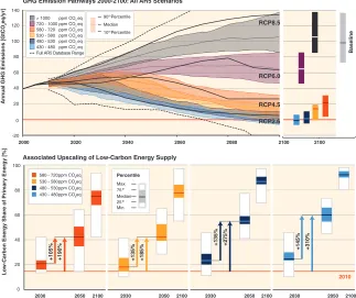
Fig. 3. – Low-carbon energy share of primary energy as a function of time and strictness of mitigation policy. For the 430–480 ppm CO2-eq scenario class (that is approximately in-line with a 2◦ target) the energy sector is almost completely decarbonized in the course of this century. Compared to 2010, in 2050 the low-carbon energy share will have 4-folded (taken from [22], fig. 4).
(3%–11%) by 2100 relative to baseline (which grows between 300% to 900% over the course of the century). This is equivalent to a reduction in consumption growth over the 21st century by about 0.06 (0.04–0.14) percentage points a year (relative to annualized consumption growth that is between 1.6% and 3% per year)(7).
In that sense, the CEA has delivered a result upon which society could move forward in the sense that was discussed at the end of the CBAvs.CEA section. However, the aca-demic debate on whether a society can easily afford such a kind of loss is still yet to come. Society might wish to exclude some mitigation options for the one or other reason (see also fig. 4). Any such exclusion represents another constraint for the economic optimization, hence the thereby obtained optimum will be even more welfare sub-optimal than the climate target-constrained solution. As a result, additional costs will occur. It turns out that the additional costs for not allowing for carbon capture and storage
430-530 ppm CO2eq Obs. 530-650 ppm CO2eq Obs. 430-650 ppm CO2eq Range
Median +1 Standard Deviation
-1 Standard Deviation
‡ Scenarios from two models reach concentration levels in 2100 that are slightly above the 430-480 ppm CO2eq category † Scenarios from one model reach concentration levels in 2100 that are slightly below the 530-580 ppm CO2eq category 530†- 580 ppm CO2eq
Scenario 430 - 480‡ ppm CO2eq
Min 75th Percentile Max
Median 25th Percentile
Mitigation Gap till 2030 [%]
0 20 40 60 80 100
-20 0 +20 +40 +60 +80 +100 +120 +160 +140 −100 −50 0 +50 +100 +150 +200 +250 +300
Mitigation Cost Incr
ease Relative to Default
Technology
Assumptions [%]
No CCS Nuclear
Phase Out Limited Solar/Wind
Limited Bioenergy
Mitigation Costs Incr
ease (% Differ
ence w.r
.t.
Immediate Mitigation)
* Number of models successfully vs. number of models attempting running the respective technology variation scenario
8/10* 12/12* 8/9* 10/10* 8/9* 10/10* 4/10* 11/11*
< 55 Gt CO2 in 2030
> 55 Gt CO2 in 2030
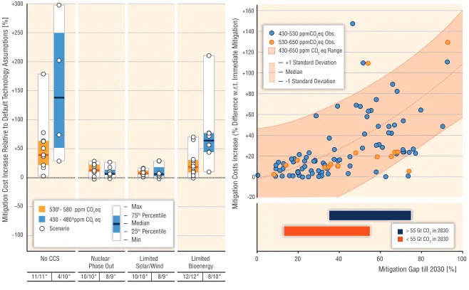
Fig. 4. – Relative increase of mitigation costs in net present value (2015–2100, discounted at 5% per year) from technology portfolio variations relative to a scenario with default technology assumptions. Scenario names on the horizontal axis indicate the technology variation relative to the default assumptions: No CCS = unavailability of CCS, Nuclear phase out = No addition of nuclear power plants beyond those under construction; existing plants operated until the end of their lifetime; Limited Solar/Wind = 20% limit on solar and wind electricity generation; Limited Bioenergy = maximum of 100 EJ/yr bioenergy supply (taken from [23], fig. 13).
(CCS) are in the order of 100%, while those for no addition of nuclear power plants beyond those under construction are an order of magnitude smaller, like for limiting solar/wind’s contribution to electricity generation to 20%. In the following sense CCS is a unique mitigation technology: it is the only one that would allow for “negative emissions” when combined with biomass conversion or other technologies that would allow for removing carbon dioxide from the atmosphere. This allows for overshooting the carbon budget in the first half of the century and compensating this overshoot by negative emissions in the second half of the century if sufficient secure geological storage volume is left to take up carbon dioxide from biomass conversion.
5. – Investment under uncertainty
One key system property that has attracted a lot of attention in the climate com-munity is the so-called climate sensitivity (CS). CS is defined as the equilibrium GMT response to a doubling of the CO2concentration as against the pre-industrial value. CS also encapsulates more than 50% of the uncertainty about future transient GMT response to greenhouse gas emissions. At present, there is no way to give an upper limit for CS on the basis of climate science [2]. An intermediate value is assumed to be 3◦C, and an at least 66% quantile 1.5◦C–4.5◦C. As one can show that the allowed time-cumulative amountE of CO2 scales with the time-asymptotic GMT [24],
(3) E∝2T∞/CS−1,
the total amount of CO2 still allowed tends to zero, as CS to infinity. This in turn means that the asymptotic GMT unavoidably would transgress 2◦C, if CS was only large enough. But then, maximum GMT would transgress 2◦C all the more so, hence from this thought experiment we conclude: As long as no upper limit can be put on CS, we cannot formulate a mitigation policy that could comply with the 2◦ limit with certainty. Instead [25] suggested a generalization of the 2◦target that involves compliance with the 2◦ limit only in a probabilistic sense. Hence, now two normative parameters have to enter the analysis: the temperature limit and the probability of observing it. When transferring this idea to CEA, one adds the notion of optimization to it, resulting in the so-called “chance constrained programming” (CCP — whereby “programming” means “optimization” [26]). CCP for the 2◦ target with a probability of compliance of 75% was implemented in the MIND model by [27]. Compared to a deterministic CEA version, investments into low-emission technologies would have been chosen decades earlier. In part this is a trivial effect, as running a deterministic CEA with mean values of uncertain quantities such as CS would roughly imply compliance with the 2◦ limit with a chance of only 1/2. When now asking for 75%, this would naturally trigger earlier investments into low-carbon technologies. However, as [27] show, this only partly explains the effect. It remains to be shown whether non-linear interactions of uncertainties in the climate and the technology module are co-responsible for this suggested massive acceleration of investments.
However, as early as 1974, Blau [28] showed that strict environmental targets might be fundamentally at odds with anticipated future learning. Schmidtet al.[29] showed that this argument readily applies to CCP regarding the climate problem: If we anticipate that we might learn in future that CS is “very high”, we anticipate a future in which we cannot reach the politically set probability of compliance any longer — or only at the price of complete shutdown of emission right away. Schmidt et al. argue that there is no obvious way to include learning into CCP of the climate problem in a self-consistent manner. Instead they suggest an alternative to CCP: the so-called cost-risk analysis (CRA).
Like CCP, CRA contains two normative parameters. Like CCP and CEA, it requests defining a temperature limit. Unlike CCP, it asks for a linear trade-off parameter that weighs mitigation costs against the probability of overshooting. The latter could be interpreted as a very special case of a generalized damage function, and in that sense we would be back to some sort of CBA. But still, no true damages need to be formulated, and in that sense one could interpret CRA as the climate-problem adjusted hybrid out of CBA and CEA under uncertainty and anticipated future learning. The properties and consequences of this new decision analytic tool are at present subject to academic investigation(8). Neuberschet al. [30] utilize a version of CRA that linearly penalizes a transgression of a temperature target. They argue it was the most conservative way to formulate a risk function that would still avoid any counterintuitive “tipping” towards a high-emission path, once a target has been missed. Then they suggest to calibrate the trade-off parameter between economic utility and climate risk such that without further anticipation of future learning about CS (a realistic assumption for the mental framing of the COP discussion process), 66% compliance with the 2◦ target is generated.
They apply this concept to the MIND model in its simplest form, distinguishing only a fossil and a renewable sector. They find: investment paths for CRA including anticipated future learning mimic those for CCP for the first half of this century. In addition, from [27] it follows that CEA can mimic CCP (up to a temporal accuracy of a decade) if the deterministic value of CS is properly chosen. The combination of both statements suggests that likely the existing 1000 IPCC-reported scenarios, mostly generated in the CEA framework, can be given a sane interpretation under CS uncertainty (hereby bravely extrapolating from the structurally much simpler MIND model): for the compliance level attached to any scenario they would tackle the extreme case of no future learning, hence their cost estimates represent upper limits while their control paths might be good approximations of the optimal paths for the next decades.
Can we obtain anything from CRA in addition to what we got from CEA? Only within CRA the question “what is the expected value of perfect climate information?” (in the sense of perfect forecast in response to carbon dioxide emissions), given a temperature target, is a well-posed one. For the first time, that question can meaningfully be answered for the 2◦ target. Depending on the setting of normative parameters of the model, it
could be up to hundreds of billions of Euro per year [30] which could be seen as an incentive to invest faster in improved climate observation and modelling systems.
Finally, does the above development of a new decision-analytic tool like CRA imply in part a “rehabilitation” of CBA from the perspective of the “CEA community”? I would say: yes. CBA can formally deal more easily with uncertainty and has even a very strong axiomatic basis: according to the von Neumann-Morgenstern axioms, under a given probability measure linking our actions to the consequences of those actions, a “rational decision-maker” would optimize expected utility (or welfare), which means in the context of the climate problem nothing else than applying a probabilistic version of CBA (as was done in a pioneering work in [10]). What would then be the effect of explicitly involving uncertainty in CBA compared to the simpler deterministic treatment? For now the effect ranges from being minuscule to a recommendation of complete shutdown of emissions right now [31] due to uncertainty. Thus, in fact, the recommendations of CBA for dealing with uncertainty appear even more unstable than the treatments of their deterministic counterparts. It remains a conceptual challenge to develop the adequate decision-analytic tool, given our present state of knowledge about the climate system. Future research needs to show to what extent CRA can serve as a bridge, representing the limiting case of learning about the climate response, but not about damages.
6. – Prospects of climate policy
While proponents of a stringent mitigation policy might see it as a success that the 2◦ target was embraced by the Conference of the Parties, binding international agreements on emission cuts dramatically lag behind this embracement (they are currently equivalent to a 2.4–4.2◦C target) (80% quantile, [32]). This has several reasons. First, the 2◦target can roughly be converted into a carbon emission budget — if this were distributed equally per capita, a citizen of the OECD would run out of emission allowances within the next decade [33]. Hence, global society has to negotiate how to distribute the remaining emission allowances. The fact that least developed nations might not be able to fully use their rights over the next decades and hence could sell those to OECD nations could mitigate part of that negotiation problem.
Secondly, a 2◦target would massively depreciate the rents of owners of fossil resources. In principle this would not have to be a problem from the point of view of the global society, however, pressure groups might use information asymmetries quite efficiently. Part of this effect is that actors in their networks hold a great deal of the necessary technological know-how to operate an energy system in a stable manner.
treaty is not the only channel towards mitigation. Coalitions of mitigation-motivated actors could be stabilized by modest border tax adjustments or club goods [34]. Also, it will certainly be possible to spell out the preference order implicit in the 2◦ target for the modified conditions and re-interpret the target in a generalized sense accordingly. I regard the new tool of CRA as promising in that respect.
Fourthly, it is at present unclear whether a low-cost low-emission energy system would work in reality, in spite of an increasing number of CEAs that claim rather low mitigation costs. Hence, it would help (from the point of view of a supporter of the 2◦ target) if OECD countries could come up with successively upscaled demonstration projects — a key role for Europe. This should be supported much more by concerted, problem-oriented efforts within academia in the techno-economic field and frontier research in social science. Now there are two interpretations of this series of obstacles for a global mitigation policy: on the one hand, one may argue that the combination of those effects makes a success of mitigation policy rather unlikely. On the other hand, this series provides an analytic explanation why we have not seen that policy yet while at the same time they provide entry points to develop policy instruments to tackle those obstacles in a targeted manner and thereby resolve the current climate policy stalemate.
In the end, climate policy will be to a large extent a matter of removing information asymmetries within our global society. If the proponents of a stringent mitigation policy are correct in that their suggestions in some sense would maximize the “global cake” (including humankind’s desire for some security standards) — then there should be some ways to negotiate fair deals. Or, quite the reverse, they may find themselves convinced that they have just followed some romantic ideal of nature conservation, out of touch with the preference order of global society. The negotiations about what a desirable and fair future is have just begun. They can be informed but not substituted by imagina-tions of a handful of well-meaning brilliant scientists. They can be massively supported by an academia that internally stronger rewards dealing with real-world problems of this century, strictly observes political neutrality, and opens up option spaces for policy makers. The climate problem is increasingly attracting curious minds from all disciplines and triggers a massive cross-fertilization of academic quality standards across disciplines. This certainly will give academia a boost and hopefully society an increased chance to negotiate what kind of future it wants — in such a way that in retrospect we would find that academia has helped society to get closer to “its social optimum”!
∗ ∗ ∗
I would like to thank B. Meyer-Schmidt for technical support.
REFERENCES
[1] Held H., Climate policy options and the transformation of the energy system, in New
Strategies for Energy Generation, Conversion and Storage, Lecture Notes of the Joint
EPS-SIF International School on Energy, edited by Cifarelli L., Wagner F. and
[2] Allen et al., IPCC Fifth Assessment Report (AR5) Climate Change 2014,http://www. ipcc.ch/report/ar5/syr/.
[3] IPCC, Summary for policymakers, in: Climate Change 2014: Impacts, Adaptation, and Vulnerability. Part A: Global and Sectoral Aspects. Contribution of Working Group II to
the Fifth Assessment Report of the Intergovernmental Panel on Climate Change, edited
byField C. B., Barros V. R., Dokken D. J., Mach K. J., Mastrandrea M. D., Bilir T. E., Chatterjee M., Ebi K. L., Estrada Y. O., Genova R. C., Girma B., Kissel E. S., Levy A. N., MacCracken S., Mastrandrea P. R. andWhite L. L. (Cambridge University Press, Cambridge, UK and New York, NY) 2014, pp. 1-32. [4] Archer D.andBrovkin V.,Clim. Change,90(2008) 283.
[5] European Commission, COM, 1 (2000).
[6] Schneider von Deimling T., Ganopolski A., Held H. and Rahmstorf S.,
Geophys.Res. Lett.,33(2006) L14709.
[7] Schellnhuber H. J.,Clim. Change,100(2010) 229. doi:10.1007/s10584-010-9838-1. [8] UNFCCC, Report of the conference of the parties on its seventeenth session (2012). [9] Meinshausen M., Meinshausen N., Hare W., Raper S. C. B., Frieler K., Knutti
R., Frame D. J.andAllen M. R.,Nature,458(2009) 1158 doi:10.1038/nature08017. [10] Nordhaus W. D.,Managing the global commons: the economics of climate change (The
MIT Press) 1994.
[11] Nordhaus W. D.,A question of balance: Weighing the options on global warming policies (Yale University Press, New Haven & London) 2008.
[12] Kunreuther H., Gupta S., Bosetti V., Cooke R., Dutt V., Ha-Duong M., Held H., Llanes-Regueiro J., Patt A., Shittu E. and Weber E., Integrated Risk and
Uncertainty Assessment of Climate Change Response Policies, in: Climate Change 2014:
Mitigation of Climate Change. Contribution of Working Group III to the Fifth Assessment
Report of the Intergovernmental Panel on Climate Change, edited by Edenhofer O.,
Pichs-Madruga R., Sokona Y., Farahani E., Kadner S., Seyboth K., Adler A., Baum I., Brunner S., Eickemeier P., Kriemann B., Savolainen J., Schl ¨omer S., von Stechow C., Zwickel T.andMinx J. C.(Cambridge University Press, Cambridge, UK and New York, NY) 2014.
[13] Dasgupta P.,J. Risk Uncertain,37(2008) 141.
[14] Stern N.,Stern Review on the Economics of Climate Change(HM Treasury) 2007. [15] Traeger C. P., CUDARE Working Paper No. 1117 (UC Berkeley) 2011.
[16] Patt A.,Rev. Policy Res.,16(1999) 104.
[17] Held H. and Edenhofer O., in Handbook of Transdisciplinary Research, edited by Hirsch Hadorn G., Hoffmann-Riem H., Biber-Klemm S., Grossenbacher-Mansuv W., Joye D., Pohl C.et al.(Springer, Heidelberg) 2008.
[18] Clarke L., Jiang K., Akimoto K., Babiker M., Blanford G., Fisher-Vanden K., Hourcade J.-C., Krey V., Kriegler E., L¨oschel A., McCollum D., Paltsev S., Rose S., Shukla P. R., Tavoni M., van der Zwaan B. C. C. and van Vuuren D. P., 2014: Assessing Transformation Pathways, in: Climate Change 2014: Mitigation of
Climate Change. Contribution of Working Group III to the Fifth Assessment Report of the
Intergovernmental Panel on Climate Change edited byEdenhofer O., Pichs-Madruga
R., Sokona Y., Farahani E., Kadner S., Seyboth K., Adler A., Baum I., Brunner S., Eickemeier P., Kriemann B., Savolainen J., Schl¨omer S., von Stechow C., Zwickel T.andMinx J. C.(Cambridge University Press, Cambridge, UK and New York, NY) 2014.
[19] Junginger M., Lako P., Lensink S., van Sark W. and Weiss M.,Climate Change
[20] Luderer G., Leimbach M., Bauer N.andKriegler E.,Description of the ReMIND-R
model - Version June 2011, from
http://www.pik-potsdam.de/research/sustainable-solutions/models/remind/REMIND Description.pdf.
[21] Nordhaus W. D., The Perils of the Learning Model for Modeling Endogenous
Technological Change, Working Paper 14638, http://www.nber.org/papers/w14638,
(National Bureau of Economic Research, Cambridge, MA) 02138 (2009).
[22] IPCC, 2014: Summary for Policymakers, in:Climate Change 2014, Mitigation of Climate Change. Contribution of Working Group III to the Fifth Assessment Report of the
Intergovernmental Panel on Climate Change edited byEdenhofer O., Pichs-Madruga
R., Sokona Y., Farahani E., Kadner S., Seyboth K., Adler A., Baum I., Brunner S., Eickemeier P., Kriemann B., Savolainen J., Schlomer S., von Stechow C., Zwickel T.andMinx J. C.(Cambridge University Press, Cambridge, UK and New York, NY) 2014.
[23] Edenhofer O., Pichs-Madruga R., Sokona Y., Kadner S., Minx J. C., Brunner S., Agrawala S., Baiocchi G., Bashmakov I. A., Blanco G., Broome J., Bruckner T., Bustamante M., Clarke L., Conte Grand M., Creutzig F., Cruz-N´u˜nez X., Dhakal S., Dubash N. K., Eickemeier P., Farahani E., Fischedick M., Fleurbaey M., Gerlagh R., G´omez-Echeverri L., Gupta S., Harnisch J., Jiang K., Jotzo F., Kartha S., Klasen S., Kolstad C., Krey V., Kunreuther H., Lucon O., Masera O., Mulugetta Y., Norgaard R. B., Patt A., Ravindranath N. H., Riahi K., Roy J., Sagar A., Schaeffer R., Schl¨omer S., Seto K. C., Seyboth K., Sims R., Smith P., Somanathan E., Stavins R., von Stechow C., Sterner T., Sugiyama T., Suh S., ¨Urge-Vorsatz D., Urama K., Venables A., Victor D. G., Weber E., Zhou D., Zou J. andZwickel T., “Technical Summary”, inClimate Change 2014: Mitigation of
Climate Change. Contribution of Working Group III to the Fifth Assessment Report of the
Intergovernmental Panel on Climate Change edited byEdenhofer O., Pichs-Madruga
R., Sokona Y., Farahani E., Kadner S., Seyboth K., Adler A., Baum I., Brunner S., Eickemeier P., Kriemann B., Savolainen J., Schl¨omer S., von Stechow C., Zwickel T.andMinx J. C.(Cambridge University Press, Cambridge, UK and New York, NY) 2014.
[24] Kriegler E. andBruckner T.,Clim. Change,66(2004) 345.
[25] Kleinen T., Stochastic Information in the Assessment of Climate Change (Universit¨at Potsdam) 2005.
[26] Charnes A.andCooper W. W.,Manage. Sci.,6(1959) 73.
[27] Held H., Kriegler E., Lessmann K.andEdenhofer O.,Energy Econ.,31(2009) 550. [28] Blau R. A.,Manage. Sci.,21(1974) 271.
[29] Schmidt M. G., Lorenz A., Held H.andKriegler E.,Clim. Change,104(2011) 783. [30] Neubersch D., Held H. and Otto A., Clim. Change, 126 (2014) 305, DOI
10.1007/s10584-014-1223-z.
[31] Weitzman M. L.,Rev. Econ. Stat.,91(2009) 1.
[32] Rogelj J., Chen C., Nabel J., Macey K., Hare W., Schaeffer M., Markmann K., H¨ohne N., Krogh Andersen K. andMeinshausen M., Environ. Res. Lett., 5(2010) 034013.
[33] Wicke L., Schellnhuber H. J. and Klingenfeld D., The 2◦ max Climate Strategy
– A Memorandum, Concise English version of PIK-Report No. 116 – updated. From