Scholarship@Western
Scholarship@Western
Electronic Thesis and Dissertation Repository
7-8-2015 12:00 AM
From Solution Into the Gas Phase: Studying Protein Hydrogen
From Solution Into the Gas Phase: Studying Protein Hydrogen
Exchange and Electrospray Ionization Using Molecular Dynamics
Exchange and Electrospray Ionization Using Molecular Dynamics
Simulation
Simulation
Robert G. McAllister
The University of Western Ontario
Supervisor Lars Konermann
The University of Western Ontario Graduate Program in Chemistry
A thesis submitted in partial fulfillment of the requirements for the degree in Master of Science © Robert G. McAllister 2015
Follow this and additional works at: https://ir.lib.uwo.ca/etd
Part of the Physical Chemistry Commons
Recommended Citation Recommended Citation
McAllister, Robert G., "From Solution Into the Gas Phase: Studying Protein Hydrogen Exchange and Electrospray Ionization Using Molecular Dynamics Simulation" (2015). Electronic Thesis and Dissertation Repository. 2938.
https://ir.lib.uwo.ca/etd/2938
This Dissertation/Thesis is brought to you for free and open access by Scholarship@Western. It has been accepted for inclusion in Electronic Thesis and Dissertation Repository by an authorized administrator of
From Solution Into the Gas Phase: Studying Protein Hydrogen Exchange and Electrospray Ionization Using Molecular Dynamics Simulation
(Thesis format: Integrated Article)
by
Robert Gordon McAllister
Graduate Program in Chemistry
A thesis submitted in partial fulfillment of the requirements for the degree of
Master of Science
The School of Graduate and Postdoctoral Studies The University of Western Ontario
London, Ontario, Canada
ii
Abstract
Here, we apply Molecular Dynamics (MD) simulations to investigate fundamental
aspects of structural mass spectrometry (MS). We first examine microscopic phenomena
underlying Hydrogen/Deuterium exchange (HDX). HDX interrogates structural dynamics
of proteins by measuring the rate of Deuterium uptake into backbone amides. We
perform microsecond MD simulations on ubiquitin to investigate this process. We find
that HDX protection often cannot be explained by H-bonding or solvent accessibility
considerations. These findings caution against non-critical use of HDX data in structural
contexts. We next use MD to examine the Electrospray ionization (ESI) mechanism of
proteins. ESI is a soft ionization technique resulting in the production of gaseous protein
ions. The mechanism of ion formation from nanometer sized droplets is unclear. We
apply a trajectory stitching MD approach to simulate protein-containing nanodroplets,
finding that natively-folded proteins remain solvated as droplets shrink. Residual charge
carriers remain following desolvation, consistent with Dole’s charged residue model.
Keywords
Proteins, Molecular Dynamics, Mass Spectrometry, Electrospray Ionization,
iii
Co
-
Authorship Statement
The work in Chapter 2 was previously published and is reprinted with permission from:
McAllister, R. G. & Konermann, L. Challenges in the Interpretation of Protein
H/D Exchange Data: A Molecular Dynamics Simulation Perspective.
Biochemistry 54, 2683–2692 (2015). Copyright 2015, American Chemical Society.
The work in Chapter 3 is being prepared for future publication:
McAllister, R. G., Metwally, H., Sun, Y. S. & Konermann, L. The Electrospray
Mechanism of Natively Folded Proteins: A Molecular Dynamics Investigation.
The original drafts of these manuscripts were prepared by the author (R.G.M.) with
subsequent revisions by the author and Dr. Lars Konermann. All simulation work
presented was performed by the author. Mass Spectrometry and Ion Mobility
Spectrometry data presented in Chapter 3 were gathered and analyzed by the author with
iv Dedication
v
Acknowledgments
First and foremost, I owe tremendous gratitude to my supervisor, Dr. Lars Konermann. I
didn’t approach Lars about joining his lab until only a couple of months before my
proposed start date in September 2013. At that point, I had already been told by several
potential supervisors that they could not accommodate me in their lab on such short
notice. Despite only knowing me from a semester-long undergraduate course several
years beforehand, Lars took a chance on me, and allowed me to join his group to begin
work in molecular dynamics simulation – an area where I had little previous experience.
Since then, he has consistently challenged me to exceed my own expectations, and to
grow in my knowledge and skills. I am a better researcher, a better communicator, and a
better person for his guidance. Working with Lars for these last two years has been a
pleasure, and I will always be grateful for the opportunity he gave me.
I also thank my colleagues from the Konermann lab for many useful discussions and
thoughtful questions over the years, as well as the help they have all leant to my research.
Siavash, who has sat a meter to my left for the past year, is probably the hardest-working
researcher I’ll ever meet, and has provided guidance and advice on innumerable
occasions; I have no doubts that he will be an excellent professor one day very soon.
Haidy has been a wonderful collaborator on several of my projects, providing top notch
experimental work to go with my simulations. I could not have completed the work in
chapter 3 without her. I also thank Sherry for her help in gathering and analyzing the ion
mobility data in chapter 3, particularly as she was writing her own thesis, at the time.
Dupe, Ming, Courtney, Lauren, Danielle, Samuel, Antony, and those mentioned above
have made my experience in the Konermann lab all the richer. I haven’t the room, here,
to give them half the thanks they deserve.
To Liz, my parents, and my late grandparents, I owe more gratitude than I could ever
fully express. I thank them for always being there, and for believing in me even when I
didn’t. This work would not have been remotely possible without their love and support.
vi
Table of Contents
Abstract ... ii
Co-Authorship Statement... iii
Dedication ... iv
Acknowledgments... v
Table of Contents ... vi
List of Tables ... x
List of Figures ... xi
List of Symbols and Abbreviations... xiii
1 Introduction ... 1
1.1 Proteins ... 1
1.2 Mass Spectrometry... 2
1.2.1 The Ion Source ... 2
1.2.2 The Mass Analyzer ... 3
1.2.3 The Detector... 6
1.3 Electrospray Ionization ... 7
1.3.1 Charged Droplets ... 8
1.3.2 ESI Mechanisms ... 9
1.4 Structural Mass Spectrometry ... 11
1.4.1 Collision-Induced Dissociation and Tandem MS ... 11
1.4.2 Covalent Labelling and Cross-Linking ... 12
1.4.3 Ion Mobility Spectrometry ... 12
1.4.4 Hydrogen/Deuterium Exchange ... 13
vii
1.5.1 Ab Initio Methods and Density Functional Theory ... 15
1.5.2 Molecular Mechanics ... 16
1.5.3 Monte Carlo Methods ... 16
1.5.4 Molecular Dynamics ... 16
1.6 Molecular Dynamics in Detail ... 16
1.6.1 Newton’s Laws and Integration Algorithms ... 17
1.6.2 Force Fields ... 21
1.6.3 Thermostats ... 27
1.6.4 Additional Considerations ... 29
1.7 Scope of the Thesis ... 32
1.8 References ... 34
2 Challenges in the Interpretation of Protein H/D Exchange Data: A Molecular Dynamics Simulation Perspective... 41
2.1 Introduction ... 41
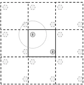
2.2 Methods... 44
2.2.1 MD Simulations ... 44
2.2.2 Data Analysis ... 44
2.3 Results and Discussion ... 46
2.3.1 Ubiquitin Structure and Dynamics... 46
2.3.2 Experimental Results ... 48
2.3.3 Main Chain H-Bonds ... 50
2.3.4 Side Chain H-Bonds ... 50
2.3.5 Solvent Accessibility ... 51
2.3.6 Unprotected Sites ... 52
2.3.7 Problem Cases ... 52
viii
2.3.9 Force Fields and Solvent Models ... 55
2.4 Conclusions ... 57
2.5 References ... 60
3 The Electrospray Mechanism of Natively Folded Proteins: a Molecular Dynamics Investigation ... 66
3.1 Introduction ... 66
3.2 Materials and Methods ... 68
3.2.1 Protein Solutions ... 68
3.2.2 Mass Spectrometry and Ion Mobility Spectrometry ... 69
3.2.3 MD Simulations: System Construction ... 69
3.2.4 MD Simulations: General Aspects ... 70
3.2.5 MD Trajectory Stitching ... 72
3.3 Results and Discussion ... 72
3.3.1 Folded Species in ESI-MS ... 72
3.3.2 Temporal Evolution of Protein Nanodroplets ... 76
3.3.3 Temperature Profile and Water Model Effects ... 78
3.3.4 Variations in Initial Protein Charge State ... 80
3.3.5 Additional Proteins ... 82
3.4 Conclusions ... 84
3.5 References ... 88
4 Conclusions and Future Work ... 93
4.1 Conclusions ... 93
4.2 Future Directions of Study ... 95
4.2.1 Extended Simulations and Additional Proteins in HDX/MS ... 95
4.2.2 Gas Phase HDX and Pulsed HDX ... 95
ix
4.2.4 Additional Macromolecules in ESI-MS... 96
4.3 References ... 97
x
List of Tables
Table 2.1 Summary of backbone NH protection behavior. ... 58
xi
List of Figures
Figure 1.1 Schematic of an ESI ion source. ... 8
Figure 1.2 Proposed models of ESI ion formation. ... 10
Figure 1.3 Interactions in a typical force field. ... 23
Figure 1.4 The Lennard Jones Potential. ... 24
Figure 1.5 The Coulombic potential for oppositely charged species... 26
Figure 1.6 Schematic of Periodic Boundary Conditions. ... 31
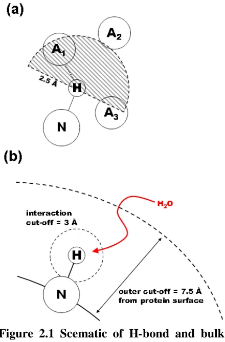
Figure 2.1 Scematic of H-bond and bulk interaction rate algorithms. ... 45
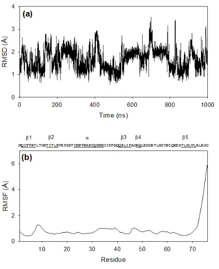
Figure 2.2 RMSD and RMSF plots for ubiquitin simulation... 46
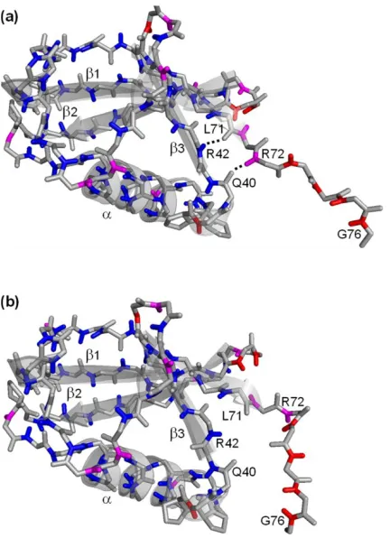
Figure 2.3 A structural fluctuation opens H-bonds near ubiquitin's C-terminus. ... 47
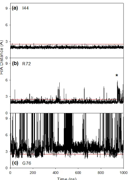
Figure 2.4 H-bonding properties of three NH sites... 48
Figure 2.5 Overview of experimental HDX data, and various properties extracted from a 1 µs CHARMM22*/TIP3P simulation. ... 49
Figure 2.6 Energy-minimized structure of ubiquitin, where blue/pink/red coloring denotes the level of HDX/NMR protection as in Figure 2.3... 51
Figure 2.7 Problem cases and waters resolved in the crystal structure. ... 53
Figure 2.8 Overview of experimental HDX data, and various properties extracted from a 1 µs Amber99sb-ILDN/TIP4P simulation trajectory. ... 56
Figure 3.1 ESI mass spectra of ubiquitin in 10 mM ammonium acetate under gentle conditions. ... 73
xii
Figure 3.3 Snapshots from a 125 ns simulation of a ubiquitin-containing nanodroplet. .. 76
Figure 3.4 Root mean square deviation of ubiquitin vs the crystal structure in an
evaporating nanodroplet... 77
Figure 3.5 Mass spectra of ubiquitin sprayed from acidified and basified solution. ... 80
Figure 3.6 Ion mobility spectra of 6+ ubiquitin ions from acidified and basified solutions.
... 81
Figure 3.7 Mass spectra of cytochrome c and holo-myoglobin at pH 7. ... 83
Figure 3.8 Snapshots from MD simulations of holo-myoglobin and cytochrome c. ... 84
Figure 3.9 Comparison of experimental data, MD simulation results and a Rayleigh
xiii
List of Symbols and Abbreviations
AMBER – Assisted Model Building with Energy Refinement
CEM – chain ejection model
CHARMM – Chemistry at Harvard Molecular Mechanics
CID – collision-induced dissociation
CRM – charged residue model
Cyt – equine heart cytochrome c
D – deuterium (2H)
DFT – density functional theory
e – the elementary charge (1.602 x 10⁻¹⁹ coulombs)
ESI – electrospray ionization
FTICR – Fourier transform ion cyclotron resonance
HDX – Hydrogen/Deuterium exchange
hMb – equine holo-myoglobin
IEM – ion evaporation model
IMS – ion mobility spectrometry
MALDI – matrix-assisted laser desorption/ionization
MD – molecular dynamics
xiv
MS/MS – tandem mass sspectrometry
m/z – mass to charge ratio
NMR – nuclear magnetic resonance
OPLS/AA – Optimized Potential for Liquid Simulation – all atom
PBC – periodic boundary conditions
PME – Particle Mesh Ewald
RF – radio frequency
RMSD – root mean square deviation
RMSF – root mean square fluctuation
SASA – solvent accessible surface area
TOF – time of flight
1
Introduction
1.1 Proteins
Proteins are a diverse class of biological macromolecules responsible for the vast
majority of physiological functions in vivo, including structural, signaling, and catalytic processes. They are polymers of amino acids ranging in size from single chains of only a
few kDa1 to multi-chain complexes of several MDa.2
The dependence of correct protein function on structure is a long-established tenet of structural biology.3-5 In the textbook example of serine protease action, the enzyme active
site contains an “oxyanion hole” positioned ideally to coordinate a tetrahedral
intermediate along the protein hydrolysis reaction coordinate. Similarly elegant
geometries are present in the active sites of enzymes ranging from lysozyme4,6 to FOF1
ATPase.7 Conversely, even small changes in the amino acid sequence of proteins –
sometimes referred to as their “primary structure” – can result in deleterious
consequences for the protein’s three-dimensional structure and function. For example, a single amino acid substitution to the oxygen carryier hemoglobin results in sickle cell
disease.8 As a result of this dependence, research on proteins often focuses on
determining both structural and dynamic properties.
X-ray crystallography remains the gold-standard technique for high-resolution protein structural determination, accounting for more than 90% of structures deposited in the
RCSB Protein Data Bank.9 High resolution structures have led to revelations in
understanding of biological systems from the first protein X-ray structure of sperm whale myoglobin10 to solving the crystal structure of the bacterial ribosome.11 Unfortunately,
many proteins cannot be purified in sufficient quantity to form suitable crystals for X-ray diffraction, are intrinsically disordered, or are otherwise not amenable to x-ray crystallography studies. Nuclear magnetic resonance (NMR) spectroscopy and
cryo-electron microscopy can obtain high-resolution structures of some of these proteins12,13 but each still requires high concentrations of homogenous sample, and also
easily obtained, one can still probe structure using lower-resolution techniques including ultraviolet-visible light spectroscopy14, circular dichroism spectroscopy15, small angle scattering experiments16, or structural mass spectrometry. Structural mass spectrometry is
a widely-applicable and highly adaptable technique which can yield a wealth of structural data17, as will be discussed below.
1.2 Mass Spectrometry
Mass spectrometry (MS) is an analytical technique that measures the mass to charge ratio
(m/z) of analyte ions, where m is the ion mass in Daltons and z is the charge in terms of the elementary charge, e. The foundations for MS were laid during J. J. Thomson’s search for the electron, and subsequent developments in the early 20th century extended
its use to characterizing isotopic distributions and identifying organic compounds.18
Further developments opened the door for MS on biological macromolecules and
structural MS studies. Today, alongside their use in traditional research environments,
MS is applied in fields as diverse as forensics19 and space exploration.20
MS is a hugely useful technique for chemical and protein analysis largely because of its
minimal analyte consumption, high sensitivity, low cost of operation, and tolerance for
non-homogenous samples. Instruments are varied, and often specialized for particular applications, but they generally consist of three components: an ion source, a mass
analyzer, and a detector. We will touch on each of these components briefly, highlighting
aspects relevant to protein MS.
1.2.1
The Ion Source
The ion source generates charged gas-phase species. Many different ionization strategies have been developed. Electron impact ionization has been in use for both solid and
gaseous analytes for nearly a century21,22, and has proven to be effective for detection and
identification of small molecules. Other techniques, including chemical ionization
approaches23 have also been successful in this area. Unfortunately, these “harsh”
ionization techniques, which rely on gas phase collisions between the analyte and
charged particles, lead to extensive fragmentation, a problem that is exacerbated for large
In order to analyze proteins via MS, researchers typically rely on one of two “soft”
ionization methods developed in the late 1980’s: matrix-assisted laser desorption/ionization (MALDI) and electrospray ionization (ESI). MALDI, developed by
Karas and Hillenkamp24, uses an ultraviolet laser to vaporize and ablate a protein
co-crystallized with an organic “matrix.” The precise mechanism of ionization in MALDI is still not comprehensively understood25, but it is known to produce intact
protein ions in the gas phase and can be tuned for resilience to the presence of
contaminants such as salt and detergent.26,27
ESI, which will be discussed in more detail below, was developed by Fenn and
co-workers.28 It relies on the production of highly-charged protein ions from charged solvent droplets. ESI has many of its own advantages for protein analysis, including its
ability to be directly coupled to upstream chromatography for efficient separation and
analysis of complex mixtures, and has become the most-used ionization technique in protein MS.29
More recently, a number of “ambient” ionization techniques have been developed for in situ analyses that require efficient ionization outside the confines of the laboratory. These include desorption electrospray ionization30 and laser ablation / electrospray ionization.31
1.2.2
The Mass Analyzer
The mass analyzer separates gas phase ions based on their m/z values. These analyzers typically consist of magnetic and electric fields forming ion “optics” which focus and
guide the analyte ions to the detector, as governed by the classical equation of motion for
ions:
𝑚 𝑧
𝒂
𝑒 =𝑬+ (𝒗 × 𝑩) (1.1)
where m is the mass of the particle, z is the ion charge in terms of the elementary charge (e), a is acceleration, E is the electric field, v is velocity, and B is the magnetic field (bolded quantities represent vectors). Equation 1.1 is derived from Newton’s second law
In order to reduce collisions with background gas molecules, prevalent at ambient
pressures, mass analyzers are housed inside a vacuum chamber held at a pressure that is
typically less than 10-6 Torr by vacuum pumps. Modern mass analyzers are able to
achieve both high sensitivity and high resolution. Capacity for tandem MS experiments,
low cost, and small size are additional desirable features in a mass analyzer.
Electric and/or magnetic sector mass analyzers were among the first to be developed32
and are still in use today. In this type of instrument, travelling ions are deflected by static
electric or magnetic fields in discrete regions of their flight path. For particles with a
known initial velocity, their deflection can be calculated precisely using equation 1.1.
These instruments are typically operated in a continuous scanning mode, which
modulates the magnitude of the electric or magnetic field to transmit only a single m/z to the detector at a given time. This scanning is highly selective, but carries the risk that
ions which are not “caught” by the specific parameters chosen will not be detected by the
instrument. Sector instruments also tend to be expensive due to the strong static magnetic
fields that they must generate and are less suitable for performing tandem MS
experiments than other platforms, resulting in their being used primarily for small
molecule analyses.
Quadrupole mass analyzers consist of four conducting cylindrical rods, which use a
combination of radio-frequency (RF) voltage and DC voltage to filter out all but a small
m/z window. The RF voltage is applied such that the potential on opposite rods is in-phase and that on adjacent rods is out-of phase. When only this RF voltage is applied, ions oscillate about the center of the quadrupole, but all are transferred through (except
for ions with very low m/z such that they impact the rods). However, when a DC voltage is applied such that opposite rods have the same potential, trajectories of ions outside a
small m/z window become destabilized, impacting the rods and not transmitting to the detector. Quadrupole mass analyzers are commonly used in protein MS because they are
inexpensive, compact, and amenable for use in tandem MS, such as in a triple quadrupole
arrangement.33 Quadrupoles analyzers are typically operated in scanning mode, similar to
Pulsed mode analyzers accept packets of ions from an upstream ion gate or directly from
a pulsed ion source such as MALDI. This type of analyzer includes time-of-flight (TOF) analyzers, Orbitrap analyzers, and Fourier transform ion cyclotron resonance (FTICR)
analyzers. The latter two operate under a similar principle, whereby ions are trapped in a
harmonic oscillating orbit passing close to a detector and inducing a current, which is
recorded and later deconvoluted using a Fourier transformation to identify the individual
m/z ratios of species in the ion packet. Orbitrap instruments use an electric field to accomplish this task34, while FTICR instruments use a strong magnetic field.35 Both can
achieve very high resolutions and mass accuracy, but require long acquisition times to do
so for large analytes, making them somewhat less useful for coupling to continuous flow
sources such as ESI. Superconducting magnets needed for the highest resolution ion
cyclotron resonance instruments are also very expensive to cool and maintain.
TOF instruments have somewhat lower resolving power than Orbitrap or FTICR
instruments, but still provide many of the same advantages, while being relatively
inexpensive. Their high duty cycle allows efficient coupling to chromatography and use
in tandem MS applications.36 TOF analyzers accelerate ions through an electric field
before allowing them to drift through a field-free region. The speed of the ions as they enter the field free region is given by:
𝐸𝑝𝑝𝑝𝑒𝑝𝑝𝑝𝑝𝑝 =𝐸𝑘𝑝𝑝𝑒𝑝𝑝𝑘 (1.2)
𝑒𝑒∆𝑈= 1
2𝑚𝑣2 (1.3)
𝑣= �2𝑒𝑧∆𝑈𝑚 (1.4)
where v is the ion speed, z is the charge in terms of the elementary charge, e, ∆U is the potential difference across the electric field, and m is the ion mass. Since particles move at a constant speed in the vacuum environment of the TOF’s field free region, flight time
can be calculated as:
where tf is the ion flight time, l is the length between the “pusher” field region and the
detector. Combining equations 1.4 and 1.5 yields:
𝑝 𝑝𝑓=�
2𝑒𝑧∆𝑈
𝑚 (1.6)
𝑡𝑓= 𝑙�2𝑒𝑧∆𝑈𝑚 =�𝑚𝑧 � 𝑝
2
2𝑒∆𝑈 (1.7)
which can be simplified to
𝑡𝑓 =�𝑚𝑧 𝑘 (1.8)
where k is a constant that is independent of the ion species. Ions with a greater m/z arrive later after the ion packet is released, and the flight time recorded can be used to
determine the m/z precisely using equation 1.8. For improved resolution, modern TOF analyzers typically employ acceleration orthogonal to the ions’ original direction of
travel. A reflectron reduces peak broadening which is encountered when ions with the
same m/z have different initial velocities. The reflectron also lengthens the ion path without substantially increasing instrument size. TOF analyzers are commonly used for
MS analysis of both proteins and small molecules.
1.2.3
The Detector
The detector is the component in a MS instrument that is responsible for recognizing the
presence of ions at a given m/z which have been separated in the mass analyzer. In instruments where ions make direct contact with the detector, such as TOF, quadrupole,
or sector analyzers, some form of electron multiplier is typically used. In these devices, a
single ion impacting the detector induces secondary emission of several electrons from
the detector surface. This multiplication of signal occurs several times over as emitted
electrons impact the multiplier again, resulting in a detectable current pulse. Modern
instruments often make use of multi-channel plates with many small electron multiplier channels due to their high signal gain, short duty cycle, and ability to resolve ions in both
instead pass between pairs of metal-plate electrodes while being trapped in the analyzer, inducing a weak AC voltage, which can be transformed into discrete m/z signals.34,35
The detector signals are digitized and recorded on a computer, which performs the
necessary mathematical transformations to calculate m/z values and intensities of ions. Many separate signals from the detector are combined to yield a full mass spectrum.
1.3 Electrospray Ionization
Electrospray ionization is a soft ionization technique, which is capable of ionizing large
proteins to very high charge states. ESI is effective for a wide range of analyte sizes,
from inorganic ions to small organic molecules to GDa proteins37, regardless of whether
these species are charged or neutral in solution. ESI-MS was first demonstrated by Dole for analyzing masses of polystyrene38, with subsequent development by Fenn and
co-workers extending the technique to other organic molecules, negatively charged analytes, and large proteins28,39,40 for which he was awarded a part of the 2002 Nobel
Prize in chemistry.29
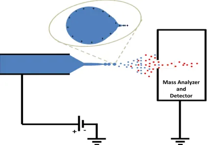
In ESI, a low-concentration protein solution is introduced into a metal capillary. A potential of several kV is applied, with the counter electrode located at the orifice of the
instrument’s mass analyzer (Figure 1.1). Electrophoretic separation of charge in the
analyte solution is driven by this potential, resulting in the formation of a Taylor cone at
the capillary tip41 as charge is accumulated and deforms the meniscus. When Coulombic
repulsion exceeds surface tension, a highly-charged jet is emitted from the Taylor cone42, which quickly deforms and disintegrates into charged droplets. Charge balance is
provided by electrolytic reactions at the capillary electrode, resulting in continuous
emission of charged droplets as long as sample is infused. Charge in these droplets is
predominantly carried by small ions including H+, Na+, Cl-, or NH4+ which were present
in the initial analyte solution. For simplicity, the remainder of the discussion on ESI will
1.3.1
Charged Droplets
Charged droplets are generated from the ESI source, carrying away a large portion of the
charge accumulated in the Taylor cone, but a comparatively small volume of sample. The
size of these droplets is strongly dependent on the size of the capillary tip, and varies
based on voltage and sample flow rate, but they are typically on the order of 10-5 m to
10-7 m range.37,43 Charge density at the surface of these droplets increases over time
concomitant with solvent evaporation, until surface tension is overcome by Coulombic
repulsion at the Rayleigh limit, which can be calculated by44:
𝑒𝑅 =8𝜋𝑒 �𝜀0𝛾𝑟3 (1.9)
where zR is the number of elementary charges, e, at the Rayleigh limit, ε0is the vacuum
permittivity, γ is the surface tension of the solvent, and r is the droplet radius.
Figure 1.1 Schematic of an ESI ion source. Taylor cones are formed at the inlet
At the Rayleigh limit, micrometer-sized droplets form Taylor cones, and emit still smaller progeny droplets, which carry away a substantial portion of the charge, but
comparatively little of the droplet volume.42,45 After this fission, both parent and progeny
droplets carry charges below the Rayleigh limit, and solvent evaporation occurs again.
Several cycles of evaporation and fission may occur, until final-generation nanometer scale droplets are produced. These final progeny droplets emit gas phase ions, which
ultimately enter the mass analyzer.
1.3.2
ESI Mechanisms
The mechanisms by which ion species are transferred from the final-generation droplets to the gas phase are still being debated.46-49 Several mechanisms have been proposed
which are relevant to the formation of gas-phase protein ions: the ion evaporation model (IEM), the charged residue model (CRM), and the chain ejection model (CEM) (Figure
1.2). All predict that ions are formed by nanometer scale droplets, but they differ in the
mechanism of ion release.
1.3.2.1
The Ion Evaporation Model
The IEM suggests that once droplets are below a radius of several nanometers, charged
ions are directly emitted from the droplet to shed charge as the surface charge density
approaches the Rayleigh limit50 (Figure 1.2a). The IEM is suspected to be the dominant
ion formation mechanism for small pre-formed ions, such as NH4+ and CH3COO- but has
also been proposed as a mechanism by which protein ions may enter the gas phase.51
Simulation studies of the ESI process have generally supported the view that IEM
pertains predominantly to small molecules.47,48,52
1.3.2.2
The Charged Residue Model
The CRM was proposed by Dole in his formative work on ESI.38 It supposes that there
exist many late-progeny droplets which contain only a single analyte ion. As solvent evaporates from these droplets, the remaining charge is left on the residual solute by
charge transfer reactions or ionic attraction, resulting in a charge state that is
This model is well supported in both experimental and simulation studies of proteins and
model polymers48,53,54, although it has not been observed directly. For small charged
NaCl clusters and solvated metal ions, the CRM has been shown to be the dominant
mechanism of ion formation by molecular dynamics simulation52,55, and it is suspected
that this mechanism will also be dominant for large, hydrophilic species, such as folded
proteins.
1.3.2.3
The Chain Ejection Model
A final model relevant to protein ion formation, the CEM, proposes that unfolded
proteins are extruded from the droplet concomitant with charging via protonation on
acidic and basic sites (Figure 1.2c). It suggests that this extension allows increased
protein charging by spreading charges apart on the extended protein chain, which extends
outside the droplet interior reducing Coulombic repulsion. Simulations using model
polymers and polyethylene glycol polymers have supported this mechanism.47,48
Figure 1.2 Proposed models of ESI ion formation. The Ion Evaporation model is
proposed for small ions (a), while the charged residue model (b) and chain ejection model (c) are proposed schemes for ionization of larger species such as proteins and polymers.
a
b
1.4 Structural Mass Spectrometry
A number of techniques exist to elucidate protein structural information using MS. These
techniques generally provide data at low-to-medium resolution, but can be informative when higher-resolution techniques are ineffective – when samples are at low concentration, are non-homogenous, or contain integral membrane and/or intrinsically disordered proteins. Many of these techniques use ESI as an ionization source due to its
compatibility with chromatographic separation and soft ionization to very high charge
states of large proteins, reducing instrument m/z range requirements.
Perhaps the simplest of these techniques is native ESI-MS, which attempt to reduce gas-phase collision and activation of proteins and protein-ligand complexes by tuning instrument parameters to lower pressures and voltages. In this way, non-covalent complexes can be preserved, and stoichiometries may be determined directly from the
mass spectrum.56,57 ESI charge state distributions can provide information about the
conformations of proteins in the sprayed solution, as a consequence of the ionization
mechanisms discussed above, with higher average charge states corresponding to
unfolded species. Analysis of these distributions can be used to probe structural
transitions, such as folding events, and even look at structural distributions in
intrinsically disordered species.17,57,58
1.4.1
Collision
-
Induced Dissociation and Tandem MS
More detailed information about analytes can be acquired by analyzing not just full
molecules, but also fragmented species by MS. Harsh ionization sources can be used to
generate these fragments in-source, but this will result in undue loss of sensitivity for protein-containing samples, due to poor selectivity and extensive fragmentation. A better approach is the use of tandem mass spectrometry (MS/MS). In MS/MS, an ion of interest
is isolated using a mass analyzer as a filter, then subjected to fragmentation before
fragments are subsequently characterized in a second mass analyzer.59
In proteins, collision-induced dissociation (CID) is often used for fragmentation. Proteins or peptides are accelerated by an electric potential in a region of the mass spectrometer
background gas result in activated species which generate ion fragments. This technique,
in combination with MS/MS, can be used to sequence and subsequently identify proteins
and peptides.60 Although collision-induced dissociation and MS/MS do not provide protein structural data directly, they can be coupled to solution or gas phase chemical
techniques such as covalent labelling and hydrogen-deuterium exchange which induce mass changes in the protein ions, yielding valuable conformational and dynamic data.
1.4.2
Covalent Labelling and Cross
-
Linking
Covalent labelling techniques, as the name implies, rely on modifying exposed region of
a protein with a reactive species such as a hydroxyl radical.61 These labels have a
predictable mass shift when measured in MS/MS, and their location gives information
about the solvent accessibility of amino acid side chains. Cross-linking studies are conceptually similar, but the reactive species is bifunctional, and therefore capable of
reacting with two protein side chains. The functional groups are typically separated by a
flexible linker, and identification of groups which have been chemically cross-linked by MS/MS can yield distance restraints which are useful in structural modelling.62
1.4.3
Ion Mobility Spectrometry
Ion mobility spectrometry (IMS) is being widely used in structural MS due to its ability
to analyze gas phase structure, and its integration into commercially available MS
instruments.63 In IMS, ions are pushed through a region containing inert background gas
by a weak electric field. Ions are accelerated at a rate proportional to charge, but
experience a “drag” force opposite their direction of travel due to the background gas. As
a result, they will move through the IMS cell at a rate that is proportional to their charge,
but inversely proportional to their collisional cross section, Ω. Compact, folded proteins have small Ω values and move through the IMS cell quickly, while large, unfolded species move more slowly.64 Recorded drift times can be compared to values calculated
from possible structures using programs such as MOBCAL65, even allowing direct ion
identification for some small species. IMS cells integrated into mass spectrometers
1.4.4
Hydrogen/Deuterium Exchange
Hydrogen/Deuterium Exchange (HDX) probes protein structure and dynamics by taking
advantage of the lability of protein O-H, S-H, and N-H bonds. When a protein is exposed to an isotopically-enriched solvent such as D2O, these labile hydrogens will be replaced
with deuterons from the solvent. This process can be monitored by MS since D is 1 Da
heavier than H, and so its incorporation into the protein results in a shift to higher m/z. NMR may also be used to monitor this process, as a result of the differing spins of the H
and D nuclei. Regardless of the instrumentation used, HDX experimentalists often seek
to obtain the rate of exchange, kHDX, which is then related to protein structure and
dynamics. Focus is usually on protein backbone amide groups which undergo HDX at a
rate that is accessible in MS and NMR.66 Exchange proceeds at each amide site
according to the Linderstrøm-Lang scheme67,68:
𝑁𝑁𝑘𝑝𝑝𝑐𝑒𝑐
𝑘𝑜𝑜𝑜𝑜
⇌
𝑘𝑐𝑐𝑜𝑠𝑜
𝑁𝑁𝑝𝑝𝑒𝑝 𝑘𝑐ℎ
→ 𝑁𝑁𝑝𝑝𝑒𝑝
𝑘𝑐𝑐𝑜𝑠𝑜
⇌
𝑘𝑜𝑜𝑜𝑜
𝑁𝑁𝑘𝑝𝑝𝑐𝑒𝑐 (1.10)
where “open” conformations are exchange-competent, while “closed” configurations are exchange-incompetent, kopen and kclose are rates of structural transition between these
states, and kch is an intrinsic rate constant which can be calculated based on the protein sequence, temperature and pD of the solution.66 The experimentally-measured exchange rate, kHDX, represents the rate of the overall conversion of NHND regardless of open or
closed state. It can be related to the fundamental HDX constants above by:
𝑐[𝑁𝐻𝑜𝑜𝑜𝑜+𝑁𝐻𝑐𝑐𝑜𝑠𝑜𝑐]
𝑐𝑝 = −𝑘𝑘ℎ[𝑁𝑁𝑝𝑝𝑒𝑝] (1.11)
𝑐𝑁𝐻𝑜𝑜𝑜𝑜
𝑐𝑝 = 𝑘𝑝𝑝𝑒𝑝[𝑁𝑁𝑘𝑝𝑝𝑐𝑒𝑐]−(𝑘𝑘𝑝𝑝𝑐𝑒+𝑘𝑘ℎ)[𝑁𝑁𝑝𝑝𝑒𝑝] (1.12)
Under equilibrium conditions, NHopenis constant, so equation 1.12 gives:
(𝑘𝑘𝑝𝑝𝑐𝑒+𝑘𝑘ℎ)�𝑁𝑁𝑝𝑝𝑒𝑝� =𝑘𝑝𝑝𝑒𝑝[𝑁𝑁𝑘𝑝𝑝𝑐𝑒𝑐] (1.13)
𝑁𝑁𝑝𝑝𝑒𝑝 =𝑘𝑜𝑜𝑜𝑜+𝑘𝑘𝑜𝑜𝑜𝑜𝑐𝑐𝑜𝑠𝑜+𝑘𝑐ℎ[𝑁𝑁𝑝𝑝𝑒𝑝+𝑁𝑁𝑘𝑝𝑝𝑐𝑒𝑐] (1.15)
Substituting equation 1.15 into equation 1.12 yields a first-order rate equation:
−𝑐�𝑁𝐻𝑜𝑜𝑜𝑜+𝑁𝐻𝑐𝑐𝑜𝑠𝑜𝑐�
𝑐𝑝 = 𝑘𝐻𝐻𝐻[𝑁𝑁𝑝𝑝𝑒𝑝+𝑁𝑁𝑘𝑝𝑝𝑐𝑒𝑐] (1.16)
where:
𝑘𝐻𝐻𝐻 =𝑘𝑜𝑜𝑜𝑜𝑘𝑜𝑜𝑜𝑜+𝑘𝑐𝑐𝑜𝑠𝑜𝑘𝑐ℎ+𝑘𝑐ℎ (1.17)
Based on the system under study, approximations can be made which allow kHDX to be
interpreted as a measure of opening free energy or kinetics. In general, kopen << kclose, and
it can be left out of the denominator of equation 1.17. For most proteins at ambient
temperature and near-neutral pH, amides spend a majority of time in the closed state, and only undergo rare, short-lived excursions to an exchange-competent structure giving the approximation kclose >> kch, in the “EX2” limiting regime and:
𝑘𝐻𝐻𝐻 =𝑘𝑘𝑜𝑜𝑜𝑜
𝑐𝑐𝑜𝑠𝑜𝑘𝑘ℎ (1.18)
allowing for estimation of the Gibbs’ free energy of the opening transition by the ratio of
observed and intrinsic exchange rates:
𝛥𝐺𝑝𝑝𝑒𝑝= −𝑅𝑅𝑙𝑅 �𝑘𝑘𝑜𝑜𝑜𝑜
𝑐𝑐𝑜𝑠𝑜𝑐�= −𝑅𝑅𝑙𝑅 �
𝑘𝐻𝐻𝐻
𝑘𝑐ℎ � (1.19)
Conversely, at high temperature or pH, the intrinsic exchange rate is elevated and
proteins may be destabilized, occupying exchange-competent states for longer periods of time in the “EX1” regime where kclose << kch. In this case, the measured rate constant
corresponds to the rate of structural opening events:
𝑘𝐻𝐻𝐻 =𝑘𝑝𝑝𝑒𝑝 (1.20)
Experimentally, in HDX/MS, these regimes are observed at a peptide level as a gradual
Mixed behavior is also possible.69 This exchange occurs as a result of individual protein
molecules exploring their full conformational space over time, allowing for the structural
transitions that underlie these HDX schemes. The m/z shift observed over time can be used to estimate the rate of exchange by measuring at multiple time points. Exchange
rates can be estimated at or near individual amide resolution using NMR, extensive
protyolytic digestion or non-ergodic fragmentation techniques such as electron capture dissociation, in MS/MS.70,71
1.5 Computer Simulations
Simulation are a useful tool for studying phenomena that are difficult or even impossible
to observe experimentally. Chemical simulations rely on computer algorithms to provide
numerical solutions to equations derived from fundamental theories. The accuracy of
these methods depends on the level of theory that is applied, but approximations are
inherent to all chemical simulations. The level of accuracy required and the size of the
system will determine which simulation strategies are employed, as greater size and
accuracy require greater computational power.72
1.5.1
Ab Initio
Methods and Density Functional Theory
Ab initio methods are based on the fundamental tenets of quantum mechanics, without input from empirical studies. These methods do not provide exact solutions to the
Schrödinger equations, but they give the closest approximations available. Hartree-Fock simulations represent a commonly used ab initio method which is based on molecular orbital theory. It makes only a few approximations about the system under study, such as
not explicitly considering electron-electron repulsion. These methods are highly computationally expensive since they include many-electron wavefunctions.72 Density Functional Theory (DFT) is somewhat less expensive, since its models are based on
single electron density rather than many-electron wavefunctions. Hybrid functional methods, which combine Hartree-Fock methods and DFT for greater accuracy with little additional computation time, have been developed73, but even the fastest of these
methods are not sufficient for simulating proteins or other large biological molecules on
1.5.2
Molecular Mechanics
Molecular mechanics is a modelling technique which can be applied to simulate large
systems such as proteins by treating the systems classically, avoiding costly quantum
mechanical calculations. Atoms are treated as the smallest unit in the simulation, and are
modelled as discrete point masses and/or charges. In these systems, potentials are
calculated from empirically- or ab initio simulation-calibrated force fields that include bonded and non-bonded interaction terms. Bonded interactions such as stretching, bending, and torsion are generally modelled through harmonic potentials, while
non-bonded interactions are modelled by various long-range potentials.72 A more detailed look at these force fields is presented in 1.6.2 Force Fields.
1.5.3
Monte Carlo Methods
Monte Carlo methods rely on random permutations of a system to generate an ensemble
of structures, whose properties and stabilities are usually determined based on molecular
mechanics force fields. The Monte Carlo simulation scheme can provide excellent
conformational sampling in protein systems, but it is limited to the study of systems at
equilibrium and no correlation to time is possible.72
1.5.4
Molecular Dynamics
Molecular Dynamics (MD) simulations are another technique that typically relies on
molecular mechanics force fields. In MD, Newton’s equations of motion are integrated
over discrete time steps to model the evolution of the simulated system over time. MD is
a preferred simulation technique for proteins because of its low computational cost,
scalability to large computer systems, and its ability to model kinetic processes.72
1.6 Molecular Dynamics in Detail
The growing use of MD simulations in recent decades is largely attributable to the wide
availability of heavily-optimized simulation programs and steadily increasing computational power that have led to the many orders of magnitude increases in both
system size and timescale accessible in MD simulation of proteins.74 The earliest protein
picoseconds75, while the state-of-the-art today includes thousands of particles simulated for several milliseconds.76
Regardless of the particulars of the system, all MD simulations share some common
features. Perhaps the most important of these features is the generation of a time-resolved trajectory of system configurations. This trajectory is a series of snapshots that
correspond to individual microstates of the system under study. At equilibrium, these
snapshots can be used to make predictions about the macroscopic system. This is due to
the ergodic principle – that is, the ensemble average (replicate microstates in simulation)
is equal to the time average (one system measured experimentally)77, provided enough
microstates are sampled. The statistical ensemble that is modelled is generally selected to
correspond to the experimental system under study. Examples include: the
microcanonical ensemble (NVE) with constant number of particles, volume, and energy,
which simulates an isolated system; the canonical ensemble (NVT) with constant number
of particles, volume, and temperature, which simulates a system in thermal equilibrium
with its surroundings; and the isothermal-isobaric ensemble (NPT), which simulates a system that is similar to NVT, but in a flexible container, such that pressure and
temperature are in equilibrium with the surroundings.
1.6.1
Newton’s Laws and Integration Algorithms
In MD, particles are treated classically, and are modelled as point masses. As a result, the
evolution of the system can be modelled using Newtonian mechanics. In particular, the
position of a particle, ri, can be fully described over the evolution of the system by
Newton’s second law:
𝑭𝑝 = −𝜕𝑼(𝒓𝜕𝒓𝒊,…,𝒓𝑵)
𝒊 = 𝑚𝑝
𝑐2𝒓𝒊
𝑐𝑝2 (1.21)
where Fi is the force on particle i, U(ri,…,rN) is the potential acting on the particle, mi is
the particle’s mass, and t is time (bolded quantities are vectors). Since forces can be calculated from the system’s current position, if it is assumed that acceleration is constant
Several different integration schemes have been developed to perform these iterative
calculations.
1.6.1.1
The Leapfrog Algorithm
With known initial conditions, an algorithm for updating positions and velocities might
consist of simple first-order approximations:
𝒓𝒊(𝑡+∆𝑡) =𝒓𝒊(𝑡) +∆𝑡𝒗𝒊(𝑡) +𝑂(∆𝑡2) (1.22)
𝒗𝒊(𝑡+∆𝑡) =𝒗𝒊(𝑡) +∆𝑡𝑭𝑚𝒊(𝑝)
𝑖 +𝑂(∆𝑡
2) (1.23)
where the O term represents a trunctation error of the indicated order (in this case Δt2). This is known as the Euler integration scheme. Unfortunately, because velocity changes
with time, equation 1.22 accumulates error quickly, since the value of the instantaneous
velocity at t is not a good estimate of the average velocity over the full timestep. In order to improve accuracy, it is preferable to expand the Taylor series in equation 1.22 to
include the second order term:
𝒓𝒊(𝑡+∆𝑡) =𝒓𝒊(𝑡) +∆𝑡𝒗𝒊(𝑡) +12∆𝑡2 𝑭𝑚𝒊(𝑝)
𝑖 +𝑂(∆𝑡
3) (1.24)
which we can rearrange to:
𝒓𝒊(𝑡+∆𝑡) =𝒓𝒊(𝑡) +∆𝑡 �𝒗𝒊(𝑡) +12∆𝑡𝑭𝑚𝒊(𝑝)
𝑖 �+𝑂(∆𝑡
3) (1.25)
In equation 1.25, we recognize the centre term as the right side of equation 1.23, but
substituting Δt for a half time step. Thus, we may write:
𝒓𝒊(𝑡+∆𝑡) =𝒓𝒊(𝑡) +∆𝑡𝒗𝒊�𝑡+12∆𝑡�+𝑂(∆𝑡3) (1.26)
Similarly, expanding equation 1.23 to include the second order term and rearranging will
yield a center term that simplifies to the acceleration (force over mass) term a
𝒗𝒊(𝑡+∆𝑡) =𝒗𝒊(𝑡) +∆𝑡 �𝑚1𝑖𝑭𝒊(𝑡) +2𝑚1𝑖∆𝑡𝑐𝑝𝑐 𝑭𝒊(𝑡)�+𝑂(∆𝑡3) (1.27)
= 𝐯𝐢(t) +∆t�m1i𝐅𝐢(t +12∆t)�+ O(∆t3) (1.28)
By substituting t=t+½ Δt:
𝒗𝒊(𝑡+32∆𝑡) =𝒗𝒊�𝑡+12∆𝑡�+∆𝑡 �𝑚1𝑖𝑭𝒊(𝑡+∆𝑡)�+𝑂(∆𝑡3) (1.29)
The Leapfrog algorithm iterates between equations 1.26 and 1.29 to update the system
over many time steps with considerably less error than the Euler algorithm.78 The
Leapfrog Algorithm gets its name from the positions/forces and velocities “hopping” one
another in each iteration, with positions and forces being updated only at full time steps,
and velocities being updated only at half-timesteps. It is an oft-used algorithm in MD because it requires only 3 calculations per iteration, making it efficient, with relatively
low error.
1.6.1.2
Verlet and Velocity Verlet Integration
The Verlet algorithm is an alternative integration scheme that was popularized by Loup
Verlet.79 It is based on the Taylor expansion of ri(t) around t±Δt:
𝒓𝒊(𝑡 − ∆𝑡) =𝒓𝒊(𝑡)− ∆𝑡𝒗𝒊(𝑡) +12∆𝑡2 1𝑚
𝑖 𝑭𝒊(𝑡)−
1 6∆𝑡3 1𝑚𝑖
𝑐
𝑐𝑝𝑭𝒊(𝑡) +𝑂(∆𝑡4) (1.30)
𝒓𝒊(𝑡+∆𝑡) =𝒓𝒊(𝑡) +∆𝑡𝒗𝒊(𝑡) +12∆𝑡2 1𝑚𝑖 𝑭𝒊(𝑡) +16∆𝑡3 1𝑚𝑖𝑐𝑝𝑐 𝑭𝒊(𝑡) +𝑂(∆𝑡4) (1.31)
Adding equations 1.30 and 1.31 yields the Verlet algorithm, after rearranging:
𝒓𝒊(𝑡+∆𝑡) +𝒓𝒊(𝑡 − ∆𝑡) = 2𝒓𝒊(𝑡) +∆𝑡2 1𝑚
𝑖𝑭𝒊(𝑡) +𝑂(∆𝑡
4) (1.32)
𝒓𝒊(𝑡+∆𝑡) = 2𝒓𝒊(𝑡)− 𝒓𝒊(𝑡 − ∆𝑡) +∆𝑡2 1𝑚𝑖𝑭𝒊(𝑡) +𝑂(∆𝑡4) (1.33)
The Verlet integration scheme is slightly more accurate than leapfrog integration, but it is
configurations of the system to begin integration, and the possibility of accumulating
round-off errors in computer systems when adding the (very small) second order term to zero-order positions stored in memory.
A more commonly used variation of the Verlet algorithm is the velocity Verlet
integration scheme:
𝒓𝒊(𝑡+∆𝑡) =𝒓𝒊(𝑡) +∆𝑡𝒗𝒊(𝑡) +12∆𝑡2 1𝑚
𝑖𝑭𝒊(𝑡) +𝑂(∆𝑡
3) (1.34)
𝒗𝒊(𝑡+∆𝑡) =𝒗𝒊(𝑡) +2𝑚1
𝑖∆𝑡(𝑭𝒊(𝑡) +𝑭𝒊(𝑡+∆𝑡)) +𝑂(∆𝑡
3) (1.35)
This algorithm solves the major issues of the Verlet scheme, but it is not as accurate. It is
very similar in performance and efficiency to the Leapfrog algorithm, but has the
advantage of calculating velocities and positions at the same time points, which is useful
in some cases. The second force calculation in equation 1.35 is typically stored in
memory for the next iteration so that expensive force calculations are performed only
once per timestep.
1.6.1.3
Energy Minimization Schemes
Energy minimization is an important step in an MD workflow, prior to the beginning of
the actual simulation. The purpose of energy minimization is to move the modelled
molecular configuration towards a local energy minimum in order to gently relax any
highly unfavourable interactions, such as non-bonded atoms overlapping, resulting in overly-large repulsive forces at the first timestep (see 1.6.2.2 Van der Waals Forces). Energy minimization is a molecular mechanics method, since it is not correlated with
time. A typical integration scheme is the method of steepest decent:
𝒓(𝑅+ 1) =𝒓(𝑅)− 𝛾𝛾𝑼(𝒓(𝑅)) (1.36)
where r(n) is a matrix containing all particle positions at step n, γ is a small, scalar distance increment, and ∇U is the gradient of the potential function. Equation 1.36 is
iterated until the potential converges to a minimum, or the maximum repulsive force in
1.6.2
Force Fields
The efficient integration of Newton’s equations in MD depends on fast computation of
potentials in a position-dependent manner. This would, ideally, be accomplished using the ab initio approaches previously discussed, but these calculations are prohibitively expensive for MD of large molecules. Instead, interactions between atoms are modelled
by “effective” potentials which are calculated by a molecular mechanics force field.
Force fields consist of a set of parameters describing the interactions between various
atom types, and a set of equations to calculate the potential based on these parameters
and the system’s state.
Force fields differ in their level of detail in describing the system and how parameters are
generated. Force fields commonly used in MD can be divided into several groups:
“all-atom” potentials, which include explicit parameters for every atom in the system; “united atom” potentials, which save computation time by including contributions from
non-polar hydrogens, such as those on methyl groups, in the parameters for the heavy atoms they are bonded to; and “coarse-grained” potentials, which reduce detail even further to improve efficiency, combining groups of heavy atoms and hydrogens into
single, large pseudo-atoms. The parameters in united-atom and coarse-grained force fields are usually fitted to reproduce experimental results. All-atom force fields may be parameterized from ab initio calculations or an empirical fitting procedure. MD simulations of proteins are often carried out with all-atom force fields, including the Optimized Potential for Liquid Simulations – All Atom (OPLS/AA) force field, which is
parameterized to fit experimental properties of liquids.80 The Chemistry at Harvard
Molecular Mechanics (CHARMM)81 and Assisted Model Building with Energy
Refinement (AMBER)82 force fields, which derive their charge parameters from density
functional theory calculations, are also common.
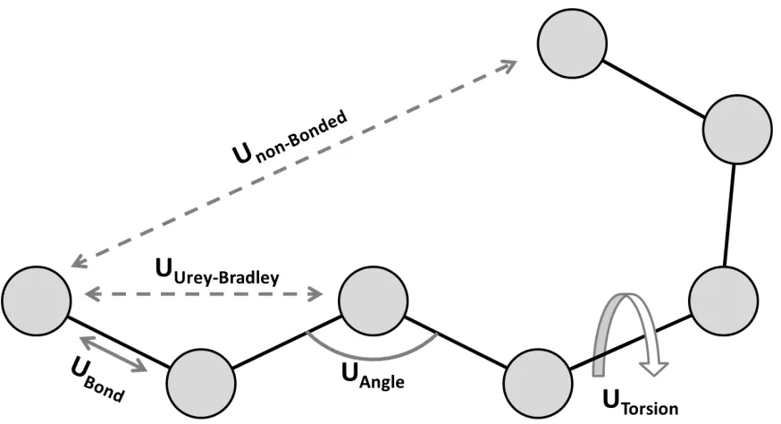
Each of these force fields contains similar sets of equations to determine the system
potential, which can be summarized as:
where the total calculated potential is a sum of bonded and non-bonded interaction terms (Figure 1.3). Non-bonded interactions are often ignored or reduced for atoms in the same molecule separated by fewer than 4 covalent bonds, as these interactions are captured by
the bonded terms. The following sections will discuss how these terms are usually
represented.
1.6.2.1
Bonded Interactions
Bonded interactions in protein MD are described in the force field by terms relating to
covalent bond stretching (2-body term), bond bending (3-body term), and dihedral torsion (4 body term). Some force fields also include additional terms, such as an
“improper” dihedral term which describes out-of-plane bending in planar systems (an additional 4-body term), or Urey-Bradley interactions which describe non-bonded force between atoms separated from one another by two covalent bonds (an additional 2-body term). The functional forms of these interactions are often based on harmonic potentials.
For example, bond stretching potential in the AMBER force field is described by81:
UBond = ∑bondskbond(d−d0)2 (1.38)
where Ubond is the contribution of bond stretching to total potential, kbond is a parameter
determined by the identity of the bonded atoms, d is the current bond length, d0 is a
parameter representing the minimum of the harmonic potential, and the sum is over all
The dihedral angles term is somewhat more complicated, because the modelled systems
may have more than one energy minimum at each bond. For example, in small
molecules, several stable rotamers, such as anti and gauche configurations, may
interconvert. In proteins, the backbone torsion angles are usually favoured to reside in
certain ranges that are determined by local secondary structure. A harmonic potential
with a single minimum would not effectively model this behavior, so the dihedral term is
usually represented by a Fourier series, as in the AMBER force field81:
𝑈𝑐𝑝ℎ𝑒𝑐𝑒𝑝𝑝 =∑𝑐𝑝ℎ𝑒𝑐𝑒𝑝𝑝𝑐 ∑𝑝𝑗=1𝑘𝑗[1 +𝑐𝑐𝑐 (𝑗𝑗 − 𝑗0,𝑗)] (1.39)
where kj and ϕ0,,j are parameters describing the amplitude and offset of the jth multiplicity
term in the Fourier series, ϕ is the current dihedral angle, and the sums are over all dihedral angles and all defined multiplicities, respectively.
Figure 1.3 Interactions in a typical force field. Bond, angle and Urey-Bradley
1.6.2.2
Van der Waals Forces
Collectively, van der Waals forces describe the interactions between molecules that are
not caused by covalent bonding or electrostatic effects. This includes permanent dipole/
permanent dipole interactions (Keesom forces), permanent dipole/ induced dipole
interactions (Debye forces), induced dipole/ induced dipole interactions (London
dispersion forces), and can be either attractive or repulsive. These interactions are usually
modelled in MD force fields using a Lennard-Jones potential80-82:
𝑈𝐿𝐿 = ∑𝑝,𝑗4𝜖 ��𝑐𝜎
𝑖,𝑗�
12
− �𝑐𝜎
𝑖,𝑗�
6
� (1.40)
where ϵ and σ are parameters which define the position and depth of the minimum in the Lennard-Jones potential, and di,j is the distance separating particles i and j. The potential
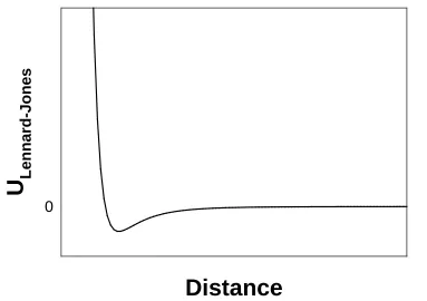
is summed over all pairs of particles to which the non-bonded interaction terms apply. The 10-6 term of the Lennard-Jones potential is attractive and there is net attraction between particles at distances past the minimum (Figure 1.4). This term approximates the
Distance
U
Le
nna
rd-J
one
s
0
Figure 1.4 The Lennard Jones Potential. Units of distance and potential are arbitrary.
averaged Keeson, Debye, and London forces. The 10-12 term is repulsive, and accounts
for the Pauli repulsion of overlapping electron orbitals at very short range (Figure 1.4).
The repulsive term can also be represented by an exponential, as in a Buckingham
potential, but the 10-12 term is often chosen for this purpose because of its fast calculation
as the square of 10-6.
The Lennard-Jones potential falls off quickly as distance between particles increases, meaning that it is often modelled with a cutoff, dc, to improve computational efficiency.
This only minimally impacts accuracy, if the cutoff is large, and a shifting adjustment is
made such that the potential equals exactly 0 at the cutoff distance:
ULJ−shifted(d) =� 0 for d > d ULJ(d)−ULJ(dc) for d≤dc
c (1.41)
1.6.2.3
Electrostatic Interactions
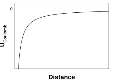
In MD, charged particle interactions are usually modelled with the Coulomb potential:
𝑈𝐶𝑝𝐶𝑝𝑝𝑚𝐶 = ∑𝑝,𝑗4𝜋𝜀𝑞𝑖0𝑞𝑐𝑗𝑖,𝑗 (1.42)
where qi and qjare the charges of particles i and j, ε0 is the vacuum permittivity, di,j is the
distance between the particles, and the sum is over all interacting pairs of particles
(Figure 1.5). Equation 1.42 is often also shifted to include a cutoff, similar to the
Lennard-Jones potential, but this may introduce problems, as the electrostatic interactions fall off much more slowly at long range. This can lead to undesirable artifacts in MD
simulations, particularly in periodic systems which simulate bulk media (discussed in
1.6.4.2 Boundary Conditions and Simulation Cells).83
A solution to this problem is modelling the long range electrostatic interactions in
periodic systems using the Ewald summation.84,85 This summation technique replaces
each point charge in the system with a point charge screened by a Gaussian charge
large distances. To compensate for these screening charges, a second Gaussian charge
distribution equal in magnitude, but opposite in sign to the screening charges is added.
Short range electrostatic contributions are calculated directly using the screened point
charges, while long range contributions can be calculated from the Fourier transform of
the compensating Gaussians. The end result is summation that rapidly converges to the
correct value for electrostatic potential, including the long range interactions.
To further improve efficiency of the Ewald summation, MD software packages often
approximate it using a Particle Mesh Ewald (PME) algorithm. PME computes the
long-range electrostatic interactions by distributing compensating charges on a discrete lattice, such that the overall charge density is maintained.86,87 In this way, the
compensating charge distribution can be computed quickly by a Fast Fourier Transform,
allowing much-improved scaling in large systems, such as proteins.
Distance
U
C
oul
om
b
0
Figure 1.5 The Coulombic potential for oppositely charged species. Units of distance
1.6.2.4
Water Models
Although implicit solvation algorithms have been developed, water is usually modelled
explicitly (i.e. as discrete particles in the system, rather than as a continuous dielectric medium). Despite the small size of H2O molecules, there are many different models to
describe them in MD, which can be classified based on the number of simulated
interaction sites, flexibility of covalent bonds, and polarizability. Polarizable and flexible
models impose additional computation costs, meaning that most protein MD studies will
benefit from use of a rigid, non-polarizable model, if it accurately reproduces properties of import.
Rigid three-site models such as TIP3P88 and SPC/E89 represent the H and O atoms explicitly with their own partial charges, and typically only consider Lennard-Jones interaction with the O atom. These models are highly efficient, and reasonably reproduce
many of the physical properties of water, such as density and diffusion coefficient.
Four-site models including TIP4P88 and its modified relative TP4P/200590 place the O charge on a massless “virtual site” that sits on the bisector of the HOH angle. These
models better reproduce experimental surface tension values relative to their three-site counterparts. Five site models that split the O charge between two virtual sites
representing lone pairs of electrons have also been developed, with sites in a tetrahedral
geometry, such as TIP5P.91 However, no model perfectly reproduces all properties of
water, and so selection of an appropriate model requires diligence on the part of the MD
practitioner.
1.6.3
Thermostats
Thermostat algorithms are used in MD simulations in order to maintain an average
temperature throughout the simulation run (for sampling in the NVT or NPT ensemble).
This is particularly desirable for systems containing large molecules, such as proteins,
since conformational changes in these molecules could otherwise lead to large
temperature fluctuations in such a small system, which is not consistent with
without a thermostat. Initial thermalization of a system is usually accomplished by
sampling velocities from a Maxwell-Boltzmann distribution, while the average temperature is maintained over time by one of several thermostat algorithms.
1.6.3.1
The Berendsen Weak Coupling Algorithm
The Berendsen thermostat is a velocity scaling scheme, which is implemented by
multiplying all particle velocities in the system by a constant, λ, determined by92:
𝜆= �1 +𝜏∆𝑝
𝑇�
𝑇
𝑇0−1� (1.43)
where ∆t is the simulation timestep,
τ
T is a coupling constant, T is the instantaneoustemperature of the system, and T0 is the thermostat’s target temperature. The square root
is taken since macroscopic temperature scales as the square of microscopic velocities.
The coupling constant describes the strength of interaction with the simulated heat bath,
with larger values producing a weaker coupling. Unfortunately, this thermostat does not
reproduce a correct NVT ensemble, partly because it does not conserve angular
momentum, however, this can be addressed by including a stochastic “noise” term in the
algorithm, at relatively little computational cost.93
1.6.3.2
The Andersen Thermostat
The Andersen thermostat is a conceptually simple algorithm for coupling to a heat bath,
and was the earliest thermostats to demonstrate NVT sampling in MD.94 In this scheme, a
subset of particles is randomly selected at each timestep, and velocities are re-sampled from a Maxwell-Boltzmann distribution for only these particles. The major shortcoming of this thermostat is that the repeated randomization of velocities results in poor
modelling of time-dependent processes in the system, such as diffusion.