Secure Two-Party Computation via Cut-and-Choose
Oblivious Transfer
∗Yehuda Lindell† Benny Pinkas‡
October 29, 2014
Abstract
Protocols for secure two-party computation enable a pair of parties to compute a function of their inputs while preserving security properties such as privacy, correctness and independence of inputs. Recently, a number of protocols have been proposed for the efficient construction of two-party computation secure in the presence of malicious adversaries (where security is proven under the standard simulation-based ideal/real model paradigm for defining security). In this paper, we present a protocol for this task that follows the methodology of using cut-and-choose to boost Yao’s protocol to be secure in the presence of malicious adversaries. Relying on specific assumptions (DDH), we construct a protocol that is significantly more efficient and far simpler than the protocol of Lindell and Pinkas (Eurocrypt 2007) that follows the same methodology. We provide an exact, concrete analysis of the efficiency of our scheme and demonstrate that (at least for not very small circuits) our protocol is more efficient than any other known today.
Keywords: secure two-party computation, malicious adversaries, cut-and-choose, concrete effi-ciency
∗
An extended abstract of this work appeared atTCC 2011. †
Dept. of Computer Science, Bar-Ilan University, Israel. [email protected]. This research was generously supported by the European Research Council as part of the ERC project LAST, and by theisrael science foun-dation(grant No. 781/07).
‡
1
Introduction
1.1 Background
Protocols for secure two-party computation enable a pair of partiesP1 and P2 with private inputs
xandy, respectively, to compute a functionf of their inputs while preserving a number of security properties. The most central of these properties are privacy (meaning that the parties learn the outputf(x, y) but nothing else),correctness(meaning that the output received is indeedf(x, y) and not something else), andindependence of inputs(meaning that neither party can choose its input as a function of the other party’s input). The standard way of formalizing these security properties is to compare the output of a real protocol execution to an “ideal execution” in which the parties send their inputs to an incorruptible trusted party who computes the output for the parties. Informally speaking, a protocol is then secure if no real adversary attacking the real protocol can do more harm than an ideal adversary (or simulator) who interacts in the ideal model [14, 15, 32, 2, 3]. An important parameter when considering this problem relates to the power of the adversary. The two most studied models are the semi-honest model (where the adversary follows the protocol specification exactly but tries to learn more than it should by inspecting the protocol transcript) and themalicious model (where the adversary can follow any arbitrary polynomial-time strategy). In the 1980s powerful feasibility results were proven, showing thatanyprobabilistic polynomial-time two-party functionality can be securely computed in the presence of semi-honest adver-saries [41] and in the presence of malicious adveradver-saries [14]. These results showed that it is possible to achieve such secure protocols, but did not demonstrate how to do so efficiently (where by effi-ciency we mean a protocol that can be implemented and run in practice). To be more exact, the protocol of [41] for semi-honest adversaries is efficient. However, achieving security efficiently for the case of malicious adversaries is far more difficult. In fact, until recently, no efficient general protocols were known at all, where a general protocol is one that can be used for computing any functionality.
This situation has changed in the past few years, possibly due to increasing interest from outside the cryptographic community in secure protocols that are efficient enough to be used in practice. The result has been that a number of secure two-party protocols were presented that are secure in the presence of malicious adversaries, where security is rigorously proven according to the aforementioned ideal/real model paradigm [23, 29, 35, 21]. Interestingly, these protocols all take novel, different approaches and so the secure-protocol skyline is more diverse than before, providing the potential for taking the protocols a step closer to very high efficiency. These protocols are discussed in more detail in Section 1.3.
1.2 Our Results
In this paper, we follow the construction paradigm of [29] and significantly simplify and improve the efficiency of their construction. The approach of [29] is to carry out a basic cut-and-choose on the garbled circuit construction of Yao [41]. (See also [33] for a different protocol based on the cut-and-choose approach, but which does not provide security according to the standard ideal/real model paradigm.) We assume familiarity with Yao’s protocol and refer to Appendix A for those not familiar. The cut-and-choose approach works by party P1 constructing s copies of a garbled
circuit and sending them toP2, who then asksP1 to open half of them in order to verify that they
are correctly constructed. If all of the opened circuits are indeed correct, then it is guaranteed that a majority of the unopened half are also correct, except with probability that is negligible in s.1 Thus,P1 andP2 evaluate the remainings/2 circuits, andP2 takes the output that appears in most
of the evaluated circuits. As discussed in [29], P2 cannot abort in the case that not all of the s/2
circuits evaluate to the same value, even though in such a case it knows that P1 is cheating. The
reason for this is that P1 may construct a circuit that computes f in the case that P2’s first bit
equals 0, and otherwise it outputs random garbage. Now, with probability 1/2 this faulty circuit is not opened and so is one of the circuits to be evaluated. In this case, if P2 would abort when
it saw random garbage then P1 would know that P2’s first input bit equals 1. For this reason, P2
takes the majority output and ignores minority values without aborting.
Although intuitively appealing, the cut-and-choose approach introduces a number of difficulties which significantly affect the efficiency of the protocol of [29]. First, since the parties need to evaluate s/2 circuits rather than one, there needs to be a mechanism to ensure that they use the same input in all evaluations (the solution for this for P2’s inputs is easy, but forP1’s inputs turns
out to be hard). The mechanism used in [29] required constructing and sending 2s2`commitments, where`is the length of P2’s input. In the implementation by [38], they useds= 160 and`= 128.
Thus, the overhead due to these consistency proofs alone is the computation and transmission of 6,553,600 commitments! Another problem that arises in the cut-and-choose approach is that a malicious P1 can input an incorrect key into one of the oblivious transfers used for P2 to obtain
the keys associated with its input wires in the garbled circuit. For example, it can set all the keys associated with 0 for P2’s first input bit to be garbage, thereby making it impossible for P2 to
decrypt any circuit if its first input bit indeed equals 0. In contrast, P1 can make all of the other
keys be correct. In this case,P1 is able to learnP2’s first input bit, merely by whether P2 obtains
an output or not. The important observation is that the checks on the garbled circuit carried out by P2 do not detect this because there is a separation between the cut-and-choose checks and the
oblivious transfer. This adversarial strategy is called a selective failure attack [24]. The solution to this problem in [29] requires making the circuit larger and significantly increasing the size of the inputs by replacing each input bit with the exclusive-or of multiple random input bits. Finally, the analysis of [29] yields an error of 2−s/17. Thus, in order to obtain an error level of 2−40 the parties need to exchange 680 circuits. We remark that it has been conjectured in [38] that the true error level of the protocol is 2−s/4; however, this has not been proven.
Our protocol. We solve the aforementioned problems in a way that is far simpler and far more efficient than in [29]. In addition, we reduce the error probability to 2−0.311s, for large enough s.
A concrete calculation yields that for an error of 2−40 it suffices to send only 132 circuits. This
1The parametersis a statistical security parameter, and it models the negligible probability that the adversary is
is an important improvement because the experiments of [38] demonstrate that the bottleneck in efficiency is not the exponentiations, but rather the number of circuits and the commitments for proving consistency. Thus, in our protocol we moderately increase the number of exponentiations, while reducing the number of circuits, completely removing the commitments, and also removing the need to increase the size of the inputs. We remark that the price for these improvements is that our protocol relies heavily on the decisional Diffie-Hellman (DDH) assumption, while the protocol of [29] used general assumptions only. We now proceed to describe our two main techniques:
1. Our solution for ensuring consistency ofP1’s inputs is to haveP1determine the keys associated
with its own input bits via a Diffie-Hellman pseudorandom synthesizer [34]. That is, P1
chooses values ga01, ga11, . . . , ga0`, ga
1
` and gr1, . . . , grs and then sets the keys associated with its ith input bit in the jth circuit to be gai0·rj, ga1i·rj. Given all of the {ga0i, ga1i, grj} values and any subset of keys of P1’s input generated in this way, the remaining keys associated
with its input are pseudorandom by the DDH assumption. Furthermore, it is possible forP1
to efficiently prove that it used the same input in all circuits when the keys have this nice structure. We stress that the garbled values for the rest of the circuit are chosen as usual. Thus, it is still possible to use garbled-circuit optimizations like that presented in [25]. 2. As we have described, the reason that the inputs and circuits were needed to be made larger
in [29] is due to the fact that the cut-and-choose circuit checks were separated from the oblivious transfer. In order to solve this problem, we introduce a new primitive called cut-and-choose oblivious transfer. This is an ordinary oblivious transfer [39, 11] with the sender inputting many pairs (x01, x11), . . . ,(x0s, x1s), and the receiver inputting many bits σ1, . . . , σs.
However, the receiver also inputs a set J ⊂ [s] of size exactly s/2. Then, the receiver obtains xσi
i for every i (as in a regular oblivious transfer) along with both values (x0j, x1j)
for every j ∈ J, while the sender learns nothing about σ1, . . . , σs and J. The use of this
primitive in our protocol intertwines the oblivious transfer and the circuit checks and solves the aforementioned problem. We also show how to implement this primitive in a highly efficient way, under the DDH assumption. We believe that this primitive is of independent interest, and could be useful in many cut-and-choose scenarios.
Efficiency analysis. Our entire protocol, including all subprotocols, is explicitly written and analyzed in a concrete and exact way for efficiency. Considerable effort has been made to optimize the constructions and reduce the constants throughout. We believe that this is of great importance when the focus of a result is efficiency. See Section 1.3 for a summary of the exact complexity of our protocol, and Section 4.3 for a complete analysis, with optimizations in Section 4.4.
Variants. Another advantage of our protocol over that of [29] is that we obtain a universally composable [4] variant that is only slightly less efficient than the stand-alone version. This is because our simulator only rewinds during zero-knowledge protocols. These protocols are also Σ protocols and so can be efficiently transformed into universally composable zero-knowledge. As with our basic protocol, we provide an explicit description of this transformation and analyze its exact efficiency. In addition, we show how our protocol yields a more efficient construction for security in the presence of covert adversaries [1], when high values of the deterrent factor are desired.
1.3 Comparison to Other Protocols
in the future. Nevertheless, as we will show, our protocol is significantly more efficient than the current best instantiations of the other approaches (at least, for not very small circuits).
• Committed input method (Jarecki-Shmatikov [23]): The secure two-party protocol of [23] works by constructing a single circuit and proving that it is correct. The novelty of this protocol is that this can be done with only a constant number of (large modulus) exponentiations per gate of the circuit. Thus, for circuits that are relatively small, this can be very efficient. However, an exact count gives that approximately 720 exponentiations are required per gate. Thus, even for small circuits, this protocol is not yet practical. For large circuits like AES with 33,000 gates, the number of exponentiations is very large (23,760,000), and is not realistic. (The authors comment that if efficient batch proofs can be found for the languages they require then this can be significantly improved. However, to the best of our knowledge, no such improvements have yet been made.)
• LEGO (Nielsen-Orlandi [35]): The LEGO protocol [35] follows the cut-and-choose method-ology in a completely different way. Specifically, the circuit constructor first sends the receiver many gates, and the receiver checks that they are correctly constructed by asking for some to be opened. After this stage, the parties interact in a way that enables the gates to be securely soldered (like Lego blocks) into a correct circuit. Since it is not guaranteed that all of the gates are correct, but just a vast majority, a fault tolerant circuit of sizeO(s· |C|/log|C|) is constructed, wheresis a statistical security parameter. The error as a function ofsis 2−sand the constant inside the “O” notation for the number of exponentiations is 32 [36]. Thus, for an error of 2−40we have that the overall number of exponentiations carried out by the parties
is 1280· |C|/log|C|. For large circuits, like that of AES, this is unlikely to be practical. (For example, for the AES circuit with 33,000 gates we have that the parties need to carry out 2,816,000 exponentiations. Observe that due to the size of the circuit, the log|C|factor is significant in making the protocol more efficient than [23], as predicted in [35]. This protocol also relies on the DDH assumption. It is worthy to note that exponentiations in this protocol are in a regular “Diffie-Hellman” group and so Elliptic curves can be used, in contrast to [23] who work in Z∗N.)
• Virtual multiparty method (Ishai et al. [21, 22]): This method works by having the parties simulate a virtual multiparty protocol with an honest majority. The cost of the protocol essentially consists of the cost of running a semi-honest protocol for computing additive shares of the product of additive shares, for every multiplication carried out by a party in a multiparty protocol with honest majority. Thus, the actual efficiency of the protocol depends heavily on the multiparty protocol to be simulated, and the semi-honest protocols used for simulating the multiparty protocol. An asymptotic analysis demonstrates that this method may be competitive. However, no concrete analysis has been carried out, and it is currently an open question whether or not it is possible to instantiate this protocol in a way that will be competitive with other known protocols.
• Cut-and-choose on circuits (Lindell-Pinkas [29]): Since this protocol has been discussed at length above, we just briefly recall that the complexity of the protocol is O(`) oblivious transfers for input-length `(where the constant inside here is not small because of the need to increase the number of P2’s inputs), and the construction and computation of s garbled
circuits and of 2s2`commitments. In addition, the proven error of the protocol is 2−s/17 and
In contrast to the above, the complexity of our protocol is as follows. The parties need to compute 15s`+ 39`+ 10s+ 6 exponentiations, where ` is the input length and s is a statistical security parameter discussed below. We further show that with optimizations the 15s` component can be brought down to just 5.66s` full exponentiations, and if preprocessing can be used then only s`/2 full exponentiations need to be computed after the inputs become known. (We remark that with preprocessing, the protocols of [35] and [21, 22] are also much more efficient.) In addition, the protocol requires the exchange of 7s` + 22`+ 7s+ 5 group elements, and has 12 rounds of communication. Finally, there are 6.5|C|s symmetric encryptions for constructing and decrypting the garbled circuits and4|C|sciphertexts sent for transmitting these circuits. An important factor here is the value of s needed. The error of our protocol is2−0.311s for large enoughs; a concrete calculation yields that for an error of 2−40 it suffices to sets= 132. (The overhead of computing an AES circuit with |C|= 33,000, `= 128 ands= 132, is therefore about 96,000 exponentiations, 28,300,000 symmetric encryptions, and communicating 270 Mbytes, where about 95% of the communication is spent on sending the garbled circuits.) Finally, we stress also that all of our exponentiations are of the basic Diffie-Hellman type and so can be implemented over Elliptic curves, which is much cheaper than RSA-type operations.
2
Preliminaries and Definitions
Throughout the paper we denote the computational security parameter byn, the statistical security parameter bys, and the length of inputs by`. The computational security parameter is the usual one that is used to model the security of the underlying computational assumptions (e.g., the DDH assumption). In contrast, the statistical security parameter models a probability of cheating that is not due to any computational hardness, but rather holds in an information-theoretic sense. For example, the probability that an adversary passes a “cut-and-choose test” depends on how large the test is and how many items are opened, but does otherwise not directly depend on computational hardness. The distinction between the two types of security parameters is important because the size of the cut-and-choose test has a dramatic effect on the efficiency of the protocol and thus the exact probability of cheating is important to analyze. For example, in our protocol, we prove that the error due to the statistical security parametersis approximately 2−0.311s. We define the notion of indistinguishability with respect to n and s, so that the error due to s is allowed only to be 2−O(s) (if this does not hold, then there is probably no reason to differentiate betweenn ands).
We consider ensembles that are indexed by integers (security parameters) n and s, and by arbitrary strings a. Security is required to hold for all a, and this value arepresents the parties’ inputs; thus, we obtain security for all inputs, and for large enough values of nand s. All parties are polynomial inn+s(and so ifais very long, a party may not be able to read all of it). Formally, we have the following definition:
Definition 2.1 Let X ={X(a, n, s)}n,s∈N;a∈{0,1}∗ and Y ={Y(a, n, s)}n,s∈
N;a∈{0,1}∗ be probability ensembles, so that for anyn, s∈Nthe distribution X(a, n, s) (resp.,Y(a, n, s))ranges over strings of length polynomial inn+s. We say that the ensembles are(n,s)-indistinguishable, denotedXn,s≡ Y, if there exists a constant 0< c≤1 such that for every non-uniform polynomial-time distinguisher
D, everys∈N, every polynomialp(·)and all large enoughn∈N, it holds that for everya∈ {0,1}∗:
Pr[D(X(a, n, s), a, n, s) = 1]−Pr[D(Y(a, n, s), a, n, s) = 1] <
1 p(n) +
1 2c·s
Definitions of security. We refer the reader to [13, Chapter 7] for the definition of security for two-party computation in the presence of malicious adversaries. The bulk of this paper is in this model. The only difference is that we require (n, s)-indistinguishability between the ideal and real distributions, rather than just regular computational indistinguishability. We also consider the models of universal composability and covert adversaries, and refer the reader to [4] and [1], respectively, for appropriate definitions.
3
Cut-and-Choose Oblivious Transfer
3.1 The Functionality and Construction Overview
Our protocol for secure two-party computation uses a new primitive that we call cut-and-choose oblivious transfer. Loosely speaking, a cut-and-choose OT is a batch oblivious transfer protocol (meaning an oblivious transfer for multiple pairs of inputs) with the additional property that the receiver can choose a subset of the pairs (of a predetermined size) for which it learns both values. This is a very natural primitive which has clear applications for protocols that are based on cut-and-choose, as is our protocol here for general two-party computation.
The cut-and-choose OT functionality, denoted Fccot, with parameter s, is formally defined in Figure 3.1, together with a variant functionality that we will need, which considers the case that R is forced to use the same choice σ in every transfer. This variant is denoted FS
ccot.
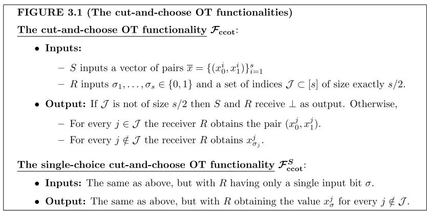
FIGURE 3.1 (The cut-and-choose OT functionalities)
The cut-and-choose OT functionalityFccot:
• Inputs:
– S inputs a vector of pairsx={(xi
0, xi1)}si=1
– R inputsσ1, . . . , σs∈ {0,1}and a set of indicesJ ⊂[s] of size exactlys/2. • Output: IfJ is not of sizes/2 thenS andR receive⊥as output. Otherwise,
– For everyj ∈ J the receiverR obtains the pair (xj0, xj1). – For everyj /∈ J the receiverR obtainsxj
σj.
The single-choice cut-and-choose OT functionality FS
ccot:
• Inputs: The same as above, but with Rhaving only a single input bitσ.
• Output: The same as above, but with Robtaining the valuexj
σ for everyj /∈ J.
In order to motivate the usefulness of this functionality, we describe its use in our protocol. Oblivious transfer is used in Yao’s protocol so that the party computing the garbled circuit (call it P2) can obtain the keys (garbled values) on the wires corresponding with its input while keeping its
input secret; see Appendix A. When applying cut-and-choose, many circuits are constructed and then half of them are opened, where opening means that P2 receives all of the input keys to the
circuit. By using cut-and-choose OT,P2 receives all of its keys in the circuits to be opened directly,
in contrast to havingP1 send them separately after the indices of the circuits to be opened are sent
fromP2 toP1. The advantage of this approach is thatP1 cannot usedifferent keys in the OT and
when opening the circuit. See Section 4.1 for discussion on why this is important.
In cut-and-choose on Yao’s protocol, one oblivious transfer is needed for every bit ofP2’s input,
that P2 uses the same input in all circuits, we use thesingle-choice variant. We present the basic
variant since it is of independent interest and may be useful in other applications.
Constructing cut-and-choose OT. The starting point for our construction of cut-and-choose OT is the universally composable protocol of Peikert et al. [37]; we refer only to the instantiation of their protocol based on the DDH assumption because this is the most efficient. However, our protocol can use any of their instantiations. The protocol of [37] is cast in the common reference string (CRS) model, where the CRS is a tuple (g0, g1, h0, h1) whereg0 is a generator of a group of
order q (in which DDH is assumed to be hard), g1 = (g0)y for some random y, and it holds that
h0 = (g0)aandh1 = (g1)b wherea6=b. We first observe that it is possible for the receiver to choose
this tuple itself, as long as it proves that it indeed fulfills the property that a 6=b. Furthermore, this can be proven very efficiently by setting b = a+ 1; in this case, the proof that b = a+ 1 is equivalent to proving that (g0, g1, h0,hg11) is a Diffie-Hellman tuple (note that the security of [37] is
based only ona6=b and not on these values being independent of each other). We thus obtain a highly efficient version of the protocol of [37] in the stand-alone model.
Next, observe that the protocol of [37] has the property that if (g0, g1, h0, h1)is a Diffie-Hellman
tuple (i.e., if a = b) then it is possible for the receiver to learn both values (of course, in a real execution this cannot happen because the receiver proves that a 6= b). This property is utilized by [37] to prove universal composability; in their case the simulator can choose the CRS so that a=b and then obtain both inputs of the sender, something that is needed for proving simulation-based security. However, in our case, we want the receiver to be able to sometimes learn both inputs of the sender. We can therefore utilize this exact property and have the receiver chooses/2 pairs (h0, h1) for which a 6= b (ensuring that it learns only one input) and s/2 pairs (h0, h1) for
which a= b (enabling it to learn both inputs by actually running the simulator strategy of [37]). This therefore provides the exact cut-and-choose property in the OT that is needed. Of course, the receiver must also prove that it behaved in this way. Specifically, it proves in zero-knowledge that s/2 out ofs pairs are such that a6=b. We show that this too can be computed at low cost using the technique of Cramer et al. [7]; see Appendix B.2 for a full description and efficiency analysis of the zero-knowledge protocol.
3.2 Background – The OT Protocol of Peikert et al. [37]
Our cut-and-choose oblivious transfer protocol is based on the oblivious transfer of [37]. Their protocol is universally composable in the common reference string model. We present an efficient instantiation of the protocol in the plain model, where there is no common reference string. This protocol is secure against malicious parties, and forms the basis for our protocol. See Protocol 3.2 for a full description.
In order to see that the receiver obtains the correct values in the last step, observe that
wσ
(uσ)r
= vσ·xσ (uσ)r
= g
s·ht·x σ
((gσ)s·(hσ)t)r
= g
s·ht·x σ
((gσ)r)s·((hσ)r)t
= g
s·ht·x σ
gs·ht =xσ.
Regarding security, if (g0, g1, h0, h1) is not a DH tuple, then the receiver can learn only one of the
sender’s inputs, since in that case one of the two pairs (u0, w0), (u1, w1) is uniformly distributed
PROTOCOL 3.2 (The Oblivious Transfer Protocol of [37] – Plain-Model Variant)
• Inputs: The sender’s input is a pair (x0, x1) and the receiver’s input is a bitσ • Auxiliary input: Both parties hold a security parameter 1n and (
G, q, g0), whereGis an efficient representation of a group of orderqwith a generatorg0, andqis of lengthn. • The protocol:
1. The receiver R chooses random values y, α0 ← Zq and sets α1 = α0+ 1. R then
computesg1= (g0)y,h0= (g0)α0 andh1= (g1)α1 and sends (g1, h0, h1) to the sender S.
2. R proves, using a zero-knowledge proof of knowledge, that (g0, g1, h0,hg11) is a DH
tuple; see Protocol B.1. ((g0, g1, h0, h1) is used as the common reference string in the
protocol of [37].)
3. Rchooses a random valuer and computesg= (gσ)randh= (hσ)r, and sends (g, h)
toS.
4. The sender operates in the following way:
– Define the function RAN D(w, x, y, z) = (u, v), where u = (w)s·(y)t and v =
(x)s·(z)t, and the values s, t←
Zq are random.
– S computes (u0, v0) =RAN D(g0, g, h0, h), and (u1, v1) =RAN D(g1, g, h1, h).
– S sends the receiver the values (u0, w0) wherew0 =v0·x0, and (u1, w1) where w1=v1·x1.
5. The receiver computesxσ =wσ/(uσ)r.
compute both inputs of the server. In order to see this, assume that σ = 0 and so g = (g0)r and
h = (h0)r. Then, it can compute x0 =w0/(u0)r as in the protocol. In addition, it can compute
x1 =w1/(u1)ry −1
. This works because w1
(u1)ry −1 =
gs·ht·x1
((g1)s·(h1)t)ry −1 =
gs·ht·x1
((g1)y −1
)s·((h 1)y
−1
)t·r =
gs·ht·x1
((g0)s·(h0)t)r
= g
s·ht·x 1
gs·ht =x1 (1)
Similarly, ifσ = 1 thenx1can be computed as in the protocol andx0 can be computed asw0/(u0)ry.
In order to prevent a malicious receiver from doing this, the zero-knowledge proof of knowledge that (g0, g1, h0,hg11) is a Diffie-Hellman tuple ensures the tuple (g0, g1, h0, h1) isnot a DH tuple, and
so the receiver can only learn a single value of the sender’s input.
The proof of security takes advantage of the fact that a simulator can extract R’s input-bit σ because it can extract the value α0 from the zero-knowledge proof of knowledge proven by R.
Givenα0, the simulator can computeα1=α0+ 1 and then check ifh=gα0 (in which case σ= 0)
or if h=gα1 (in which case σ = 1). For simulation in the case thatS is corrupted, the simulator
sets α0 = α1 and cheats in the zero-knowledge proof, enabling it to extract both sender inputs.
For the sake of completeness, we present a zero-knowledge proof of knowledge for DH tuples in Protocol B.1 in Appendix B.
3.3 Constructing a Cut-and-Choose OT Protocol
The idea behind the cut-and-choose OT protocol is essentially to run s copies of Protocol 3.2 in parallel, with the following important modification. Instead of requiring that (g0, g1, h0, h1) not be
a DH tuple in any of the executions, we actually allow the receiver to chooses/2 of the executions in which it can set (g0, g1, h0, h1) to actually be a DH tuple. This means that in these executions,
the receiver obtains both of the sender’s inputs. Of course, this must be done without the sender knowing for which of the executions the tuple is of the DH type and for which not. This is achieved by applying the methodology of Cramer et al. [7] for proving a compound statement to the basic DH zero-knowledge proof. The result is surprisingly efficient, and is described in Protocol B.2 in Appendix B. The construction of cut-and-choose OT is described in Protocol 3.3.
PROTOCOL 3.3 (Cut-and-Choose Oblivious Transfer)
• Inputs: The sender’s input is a vector ofs pairs (xj0, xj1) and the receiver’s input is com-prised ofsbitsσ1, . . . , σsand a setJ ⊂[s] of size exactlys/2.
• Auxiliary input: Both parties hold a security parameter 1n and (
G, q, g0), whereGis an efficient representation of a group of orderqwith a generatorg0, andqis of lengthn. • Setup phase:
1. Rchooses a randomy←Zq and sets g1= (g0)y.
2. For every j ∈ J, R chooses a random αj ← Zq and computes hj0 = (g0)αj and hj1= (g1)αj.
3. For every j /∈ J, R chooses random αj ← Zq and computes h j
0 = (g0)αj and h j 1 =
(g1)αj+1.
4. Rsends (g1, h10, h11, . . . , hs0, hs1) toS
5. R proves using a zero-knowledge proof of knowledge to S that s/2 of the tu-ples (g0, g1, h
j 0,
hj1
g1) are DH tuples. (R must actually prove that s/2 of the tuples
(g0, g1, h j 0, h
j
1) arenot DH tuples. In order to do this, it proves that the corresponding
tuples (g0, g1, hj0, h j
1/g1) are Diffie-Hellman tuples.) See Protocol B.2 in Appendix B.
IfS rejects the proof then it outputs⊥and halts.
• Transfer phase (repeated in parallel for every j):
1. The receiver chooses a random valuerj←Zqand computes ˜gj= (gσj)
rj,˜hj= (hj σj)rj.
It sends (˜gj,˜hj) to the sender.
2. The sender operates in the following way:
– Define the function RAN D(w, x, y, z) = (u, v), where u = (w)s·(y)t and v =
(x)s·(z)t, and the values s, t←
Zq are random.
– S sets (uj0, vj0) =RAN D(g0,g˜j, hj0,˜hj), and (uj1, v j
1) =RAN D(g1,g˜j, hj1,h˜j).
– S sends the receiver the values (uj0, w0j) wherewj0 =vj0·xj0, and (uj1, w1j) where wj1=vj1·xj1.
• Output:
1. For everyj (bothj∈ J andj /∈ J), the receiver computesxjσj = wj
σj (ujσj)rj.
2. For everyj∈ J, the receiver also computesxj1−σ j =
wj 1−σj
(uj1−σj)rj·z, wherez=y
−1modq
The security of the protocol is stated in the following proposition.
Proposition 3.4 If the Decisional Diffie-Hellman assumption holds in the group G, then
Proto-col 3.3 securely realizes the Fccot functionality in the presence of malicious adversaries.
Proof: LetAbe an adversary that controls R. We construct a simulatorS that invokesAon its input and works as follows:
1. S receives g1 and (h10, h11, . . . , hs0, hs1) from A and verifies the zero-knowledge proof as the
honest sender would.
(a) If the verification fails,S sends ⊥to the trusted party computing Fccot and halts.
(b) Otherwise,S runs the extractor that is guaranteed to exist for the proof of knowledge, and extracts a witness set {(ij, αij)} such that for every ij it holds that h
ij
0 = (g0)αij
and hi1j = (g1)αij+1. S defines the set J to be all of the indices not in the obtained
witness set. (Note that when a pair hij
0, h ij
1 is as above, thenA can obtain only one of
the strings. Thus, the setJ of the indices where Areceives both strings are those that are not included in this witness set.)
(We remark that the above procedure does not guarantee thatSruns in expected polynomial-time. Thus, formally S runs the witness-extended emulator of [26] that achieves the above effect.)
2. S receives (˜g1,˜h1), . . . ,(˜gs,h˜s) fromA.
3. For everyj /∈ J, simulatorShas obtainedαj. Sthen setsσj = 0 if ˜hj = (˜gj)αj, and otherwise
setsσj = 1.
4. For every j∈ J,S setsσj arbitrarily; say to equal 0.
5. S sends J and σ1, . . . , σs to the trusted party. Then,
(a) For every j∈ J,S receives back a pair (xj0, xj1) (b) For every j /∈ J,S receives backxjσj
6. S concludes the execution by computing RAN D as the honest sender would. Then,
(a) For everyj∈ J,S computes (uj0, w0j) and (uj1, wj1) exactly like the honest sender (it can do this because it knows bothxj0 and xj1).
(b) For every j /∈ J, S computes (ujσj, w
j
σj) like the honest sender using x
j
σ, and sets
(uj1−σ j, w
j
1−σj) to be random elements ofG.
7. S sends all of these values to A and outputs whateverAoutputs.
If the extraction of the witness set succeeds wheneverAsucceeds in proving the zero-knowledge proof, the output of the ideal execution withS isidentical to the output of a real execution withA and an honest sender. This is due to the fact that the only difference is with respect to the way the (uj1−σ
j, w
j
1−σj) are formed. However, if (g0, g1, h
j 0,
hj1
g1) is a Diffie-Hellman tuple, then (g0, g1, h j 0, h
j 1)
is not a Diffie-Hellman tuple. Now, ifσj = 0 then ˜hj = (˜gj)αj where hj0 = (g0)αj. This therefore
yields a uniformly distributed pair (uj1, wj1). (Likewise, if σ = 1 we obtain thatRAN D applied to (uj0, wj0) is uniformly distributed.) We conclude that the uniform choice of the pair (uj1−σ
j, w
j 1−σj) by S yields exactly the same distribution as in a real execution. The proof of this corruption case is concluded by noting that the probability that S does not succeed in extracting a witness when A successfully proves is negligible.
We now proceed to the case that Acontrols the sender. We construct a simulatorS as follows:
1. S computes g1 = (g0)y for a random y ← Zq, and chooses random values (hj0, hj1) so that
(g0, g1, hj0, h j
1) is a Diffie-Hellman tuplefor every j, and sends the values to A.
2. S runs the simulator for the zero-knowledge proof of knowledge with the residual A as the verifier.
3. For every j,S computes ˜gj = (g0)rj and ˜hj = (h0)rj and sends the pairs (˜gj,˜hj) to A.
4. Upon receiving back pairs (uj0, wj0) and (uj1, wj1), S computes xj0 = w j
0
(uj0)rj and x j
1 =
w1j (uj1)rj·z
wherez=y−1 modq; see Eq. (1).
5. S sends all pairs (xj0, xj1) to the trusted party, outputs whateverA outputs, and halts.
There are two main observations regarding the simulation. First, since all the (g0,g˜j, h0,˜hj)
and (g1,˜gj, h1,˜hj) tuples are Diffie-Hellman tuples, S learns all of the correct (xj0, x j
1) values that
the honest receiver would receive in a real execution. Second, by the Decisional Diffie-Hellman assumption, the output of a simulated execution with S in the ideal model is indistinguishable from the output of a real execution between A and an honest receiver. Formally, we begin with a real execution between the receiver R and A. Then, we modify R to be a simulator S1 that
works exactly asR does except that instead of honestly proving the zero-knowledge proof, it runs the simulator instead. By the zero-knowledge property, the outcome of the two executions is indistinguishable. Next, we modify S1 to S2 by having S2 work in the same way except that it
generates all of thehj0, hj1 pairs so thathj0 = (g0)αj and hj1 = (g1)αj (forall j). The fact that these
executions are indistinguishable is due to the DDH assumption. In particular, since the receiver only uses the knowledge of αj to prove the zero-knowledge proof, both S1 and S2 can run their
executions without knowing theαj values at all, and even when they receive all of thehj0, hj1 values
as external input. A direct reduction to the DDH problem is then straightforward, and is thus omitted. Finally, we modify S2 toS3 who instead of outputting the values as the receiver would
compute them, it extracts the pair (xj0, xj1) as the simulatorSwould and sets the receiver’s output to bexjσj. SinceS extracts the values in the same way as the honest receiver, this makes no difference to the output. Finally, we modify S3 to S4 by having it compute ˜gj = (g0)rj and ˜hj = (h0)rj
irrespective of the real input σj. The output distribution generated by S4 is indistinguishable to
that generated by S3 by another direct reduction to the DDH problem. We conclude by noting
that the distribution generated by S4 is identical to that generated by S in an ideal execution; specifically, it makes no difference if (xj0, xj1) are sent to the trusted party who then sends xjσj to the receiver, or if S4 sets the receiver’s output directly to xjσj.
the exchange of 6s group elements. Finally, the number of rounds remains unchanged at 6. In summary, there are 20.5s+ 5 exponentiations, 11s+ 5 group elements sent and6 rounds of communication.
3.4 Single-Choice Cut-and-Choose Oblivious Transfer
The protocol for achieving the single-choice cut-and-choose OT functionalityFS
ccot implements the
functionality that is defined formally in Figure 3.1; an intuitive description is provided in Figure 3.5.
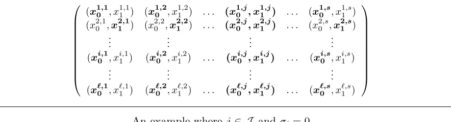
FIGURE 3.5 (Single-Choice Cut-and-Choose OT)
The inputs of the sender are depicted below. The values learned by the receiver are marked in bold. For everyj∈ J the receiver learnsboth values (xj0, xj1). In all pairs, the receiver learns one of the values, depending onσ. In the example hereσ= 0 and so the zero-values are in bold in all
pairs.
(x10, x11) (x20, x
2
1) . . . (x
j
0, x
j
1) . . . (x
s
0, x
s 1)
An example wherej ∈ J andσ = 0.
The protocol FS
ccot is achieved by modifying Protocol 3.3 above in Step 1 of the transfer phase
so that the receiverR proves that it used the same σ in every tuple. In order to enable this proof to be carried out efficiently, we modify Step 1 of the transfer phase of Protocol 3.3 as follows:
The receiver chooses a (single) random valuer ←Zq and computesg0 = (gσ)r. Then,
for every j, it computeshj = (hjσ)r. It sends (g0, h1, . . . , hs) to the sender, and proves
in zero-knowledge that it computed this correctly.
The required zero-knowledge proof is that there exists an r ∈ Zq such that either g0 = (g0)r and
hj = (hj0)r for every 1≤j≤s, org0 = (g1)r and hj = (h1j)r for every 1≤j≤s. Equivalently, the
required zero-knowledge proof is that either all of {(g0, g0, hj0, hj)}sj=1 are Diffie-Hellman tuples, or
all of{(g1, g0, hj1, hj)}sj=1are Diffie-Hellman tuples. Thus, the zero-knowledge proof of Protocol B.4
in Appendix B.3 can be used at the exact additional cost ofs+18 exponentiations and the exchange of 10 group elements (no additional rounds are needed because this proof can be carried out in parallel to the proof in the setup phase). By the soundness of the zero-knowledge proof, R must use the same σ in every transfer. The other difference in the protocol is that instead of sending a different (gj, hj) pair for everyj, the receiver sends a single valueg0. In the proof below, we show
that this does not leak any information to the sender.
Proposition 3.6 If the Decisional Diffie-Hellman assumption holds in the groupG, then the
mod-ified protocol for single-choice cut-and-choose oblivious transfer, securely realizes theFS
ccot
function-ality in the presence of malicious adversaries.
Proof: The proof is identical to the proof of Proposition 3.4, except for the following modification. When analyzing the case that the adversary controls the sender, the proof of Proposition 3.4 describes a sequence of simulatorsS1, . . . ,S4, which replace the operation of the receiver. We use the same simulators except for simulatorS4. This simulator now replaces the message (g0, h1, . . . , hs) =
((gσ)r,(h1σ)r, . . . ,(hsσ)r)), with the message ((g0)r,(h10)r, . . . ,(hs0)r)), regardless of the value of σ.
It must be shown that the distributions of these two messages are indistinguishable by the sender. Note that the sender also receives the values of the setS= (g0, g1, h10, h11, . . . , hs0, hs1), where∀j h
j 0=
(g0)αj, hj1 = (g1)αj. (In the original protocol,hj1 can also be equal to (g1)αj+1, but in simulatorsS2
Reordering the items in S, we can define it asS =S0∪S1 where Sb = (gb,(gb)α1, . . . ,(gb)αs),
for b = 0,1. Let us denote by Sr
b the set Sbr = ((gb)r,(gb)α1r, . . . ,(gb)αsr). Note that S0r and S1r
have exactly the same distribution when r is chosen at random. The sender receives eitherhS, S0ri orhS, S1ri, and therefore cannot distinguish between these two options.
Exact efficiency. The efficiency of this protocol is the same as above except for the following two changes: (1) There is no need to compute s different gj values (a single g0 is computed),
and therefore s−1 exponentiations are eliminated. (2) An additional s+ 18 exponentiations and the exchange of 10 additional group elements are needed for the zero-knowledge protocol. We therefore have 20.5s+ 24 exponentiations,11s+ 15 group elements sent and6 rounds of communication.
3.5 Batch Single-Choice Cut-and-Choose OT
In our protocol we need to carry out cut-and-choose oblivious transfers for all wires in the circuit. Furthermore, it is crucial that the subset of indices for which the receiver obtains both pairs is the same in all transfers. We call a functionality that achieves this “batch single-choice cut-and-choose OT” and denote it FccotS,B. The functionality is formally defined in Figure 3.7, and an example is given in Figure 3.8.
FIGURE 3.7 (The Batch Single-Choice Cut-and-Choose OT FunctionalityFccotS,B)
• Inputs:
– S inputs `vectors of pairs ~xi of length s, fori = 1, . . . , `. (Every vector is a row of spairs. There are ` such rows. This can be viewed as an `×s matrix of pairs; see Figure 3.8.)
– Rinputsσ1, . . . σ`∈ {0,1}and a set of indicesJ ⊂[s] of size exactlys/2. (For every
row the receiver chooses a bitσi. It also choosess/2 of the s“columns”.) • Output: IfJ is not of sizes/2 thenS andRreceive for output⊥. Otherwise,
– For every i = 1, . . . , ` and for every j ∈ J, the receiver R obtains the jth pair in vector~xi. (For every column inJ, the receiver obtains the two items of every pair,
in all rows.)
– For everyi= 1, . . . , `, the receiver R obtains theσi value in every pair of the vector ~
xi. (For every column not inJ, the receiver obtains its choice σi of the two items in
FIGURE 3.8 (Batch Single-Choice Cut-and-Choose OT)
Let the matrix below denote the inputs of the sender. Then, forj ∈ J the receiver learns both values in the jth column (values in bold). Furthermore, in each row, the receiver learns one of the values, depending on the receiver input associated with that row. For example, in theith row in the example hereσi= 0 and so the zero-values are in bold in theith row.
(x10,1, x1,11 ) (x10,2, x1,21 ) . . . (x10,j, x11,j) . . . (x10,s, x1,s1 ) (x2,10 ,x21,1) (x2,20 ,x21,2) . . . (x20,j, x21,j) . . . (x2,s0 ,x21,s)
..
. ... ... ...
(xi,01, xi,11 ) (xi,02, xi,21 ) . . . (xi,j0 , xi,j1 ) . . . (xi,s0 , xi,s1 ) ..
. ... ... ...
(x`,01, x`,11 ) (x`,02, x`,21 ) . . . (x`,j0 , x`,j1 ) . . . (x`,s0 , x`,s1 )
An example wherej∈ J and σi= 0.
In order to realize this functionality it suffices to run the setup phase of Protocol 3.3 once, and then the transfer phase of the protocol with single choice ` times in parallel (with receiver inputs σ1, . . . , σ` where σi is the receiver’s choice in execution i). This ensures that the same set
J is used in all transfers, sinceJ depends only on the values sent in the setup phase. We remark that parallel composition holds here because the simulation only rewinds in the transfer phase for the zero-knowledge protocol, and Protocol B.2 that forms the basis of the zero-knowledge proof is zero-knowledge under parallel composition (as stated in Proposition B.3).
Proposition 3.9 Assuming that the Decisional Diffie-Hellman assumption holds in G, the
above-described protocol securely realizes FccotS,B in the presence of malicious adversaries.
Exact efficiency. The setup phase here remains the same, and including the zero-knowledge costs 9s+ 5 exponentiations and the exchange of 5s+ 5 group elements. The transfer phase is repeated `times, where each transfer incurs a cost of 11.5s+ 19 exponentiations and the exchange of 5s+ 11 group elements. We conclude that there are 11.5s`+ 19`+ 9s+ 5 exponentiations, 5s`+ 11`+ 5s+ 5 group elementssent and 6 rounds of communication. In Section 4.4 we observe that 9.5s`of the exponentiations are “fixed-base” and thus this can actually be reduced to the equivalent of 5.166s` exponentiations.
4
The Protocol for Secure Two-Party Computation
4.1 Protocol Description
Before describing the protocol in detail, we first present an intuitive explanation of the different steps, and their purpose:
Step 1: P1 constructs s copies of a Yao garbled circuit for computing the function. The keys
(garbled values) on the wires of thescopies of the circuit are all random, except for the keys corresponding to P1’s input wires, which are chosen in a special way. Namely, P1 chooses
random valuesa01, a11, . . . , a0`, a`1 (where the length of P1’s input is `) andr1, . . . , rs, and sets
the keys on the wire associated with its ith input in the jth circuit to be ga0i·rj and ga1i·rj. Note that the 2`+svaluesga01, ga11, . . . , ga0`, ga
1
`, gr1, . . . , grs constitute commitments to all 2`s keys.2 (The keys are actually a pseudorandom synthesizer [34], and therefore if some of the keys are revealed, the remaining keys remain pseudorandom.)
2
Step 2: The parties execute batch single-choice cut-and-choose OT.P1 inputs the key-pairs for all
wires associated withP2’s input, andP2inputs its input and a random setJ ⊂[s] of sizes/2.
The result is thatP2learns all the keys on the wires associated with its own input fors/2 of the
circuits as indexed byJ (called check circuits), and in addition learns the keys corresponding to its actual input in these wires in the remaining circuits (called evaluation circuits). Step 3: P1 sends P2 the garbled circuits, and the values ga
0
1, ga11, . . . , ga0`, ga1`, gr1, . . . , grs which are commitments to all the keys on the wires associated with P1’s input. At this stage P1 is
fully committed to all scircuits, but does not yet know which circuits are to be opened. Step 4: P2 reveals to P1 its choice of check circuits and proves that this was indeed its choice by
sendingboth values on the wire associated withP2’s first input bit in each check circuit. Note
thatP2 can know both these values only for circuits that are check circuits.
Step 5: To completely decrypt the check circuits in order to check that they were correctly con-structed,P2 also needs to obtain all the keys on the wires associated withP1’s input.
There-fore, if thejth circuit is a check circuit,P1 sendsrj toP2. Given all of thega 0
i, ga
1
i values and rj,P2can compute all of the keysga
0
i·rj, ga1i·rjin thejth circuit by itself (andP
1cannot change
the values). Furthermore, this reveals nothing about the keys in the evaluation circuits. Step 6: Given all of the keys on all of the input wires, P2 checks the validity of the s/2 check
circuits. This ensures thatP2will catchP1with high probability if many of the garbled circuits
generated byP1 do not compute the correct function. Thus, unless P2 detects cheating, it is
assured that a majority of the evaluation circuits are correct.
Step 7: All that remains is for P1 to send P2 the keys associated with its actual input, and then
P2 will be able to compute the evaluation circuits. This raises a problem as to howP2 can be
sure thatP1 sends keys that correspond to the same input in all circuits. This brings us to the
way thatP1 chose these keys (via the Diffie-Hellman pseudorandom synthesizer). Specifically,
for every wire i and evaluation-circuit j, party P1 sends P2 the value ga
xi
i ·rj where x
i is the
ith bit of P1’s input. P1 then proves in zero-knowledge that the same axii exponent appears
in all of the values sent. Essentially, this is a proof that the values constitute an “extended” Diffie-Hellman tuple and thus this statement can be proven very efficiently.
Step 8: Finally, given the keys associated with P1’s inputs and its own inputs, P2 evaluates the
evaluation circuits and obtains their output values. Recall, however, that the checks above only guarantee that a majority of the circuits are correct, and not that all of them are. Therefore, P2 outputs the value that is output from the majority of the evaluation circuits.
We stress that if P2 sees different outputs in different circuits, and thus knows for certain
thatP1 has tried to cheat, it must ignore this observation and output the majority value (or
otherwise it might leak information to P1, as in the example described in Section 1.2).
hash function suffices for this [6, 18]. The only subtlety is thatP1 must be fully committed to the garbled circuits, including these symmetric keys, before it knows which circuits are to be checked. However, randomness extractors are not 1–1 functions. This is solved by havingP1 send the seed for the extractor before Step 4 below. Observe that the{ga0
PROTOCOL 4.1 (Computingf(x, y))
Inputs: P1 has inputx∈ {0,1}`andP2 has inputy∈ {0,1}`.
Auxiliary input: a statistical security parameters, the description of a circuitC such thatC(x, y) = f(x, y), and (G, q, g) whereGis a cyclic group with generatorgandprime orderq, andqis of lengthn.
The protocol:
1. Input key choice and circuit preparation:
(a) P1chooses random valuesa01, a11, . . . , a0`, a`1∈RZq andr1, . . . , rs∈RZq.
(b) Letw1, . . . , w`be the input wires corresponding toP1’s input inC, and denote bywi,j the
instance of wirewi in the jth garbled circuit, and byki,jb the key associated with bitbon
wirewi,j. Then,P1sets the keys for its input wires to:
ki,j0 =H(ga
0
i·rj) and k1
i,j=H(ga
1 i·rj)
whereH is a suitable randomness extractor [6, 18]; see also [10].
(c) P1 constructssindependent copies of a garbled circuit of C, denotedGC1, . . . , GCs, using
random keys except for wiresw1, . . . , w`for which the keys are as above; see Appendix A.
2. Oblivious transfers: P1andP2 run batch single-choice cut-and-choose oblivious transfer (Pro-tocol 3.7), with parameters `(the number of parallel executions) and s (the number of pairs in each execution):
(a) P1defines vectors~z1, . . . ~z`so that~zicontains thespairs of random symmetric keys associated
withP2’sith input bityiin all garbled circuitsGC1, . . . , GCs.
(b) P2 inputs a random subset J ⊂[s] of size exactlys/2 and bitsσ1, . . . , σ`∈ {0,1}, where
σi=yifor everyi.
(c) P2 receives all the keys associated with its input wires in all circuits GCj forj ∈ J, and
receives the keys associated with its inputyon its input wires in all other circuits.
3. Send circuits and commitments: P1 sends P2 the garbled circuits (i.e., the gate and output tables), the “seed” for the randomness extractorH, and the following “commitment” to the garbled values associated withP1’s input wires:
n
(i,0, ga0i),(i,1, ga1i) o`
i=1
and n(j, grj)os j=1
4. Send cut-and-choose challenge: P2sendsP1the setJ along with thepair of keys associated with its first input bity1in every circuitGCjforj∈ J. If the values received byP1are incorrect, it outputs⊥and aborts. CircuitsGCjforj∈ J are calledcheck-circuits, and forj /∈ J are called evaluation-circuits.
5. Send all input garbled values in check-circuits: For every check-circuit GCj, party P1 sends the value rj to P2, and P2 checks that these are consistent with the pairs {(j, grj)}j∈J received in Step 3. If not,P2 aborts outputting⊥.
6. Correctness of check circuits: For every j ∈ J, P2 uses thega 0
i, ga1i values it received in Step 3, and the rj values it received in Step 5, to compute the values ki,j0 = H(ga
0 i·rj), k1
i,j =
H(ga1i·rj) associated withP
1’s input inGCj. In addition it sets the garbled values associated with
its own input inGCjto be as obtained in the cut-and-choose OT. Given all the garbled values for
all input wires inGCj, partyP2 decrypts the circuit and verifies that it is a garbled version ofC. If there exists a circuit for which this does not hold, thenP2 aborts and outputs⊥.
7. P1 sends its garbled input values in the evaluation-circuits:
(a) P1sends the keys associated with its inputs in the evaluation circuits: For everyj /∈ J and every wirei= 1, . . . , `, partyP1 sends the valuek0i,j=ga
xi i ·rj;P
2 setski,j=H(k0i,j).
(b) P1 proves that all input values are consistent: For every input wirei = 1, . . . , `, party P1 uses Protocol B.4 to provein parallelthat there exists a valueσi∈ {0,1}such that for every
j /∈ J, k0i,j =ga σi
i ·rj. (Namely, it proves that all garbled values of a wire are of the same bit.) If any of the proofs fail, thenP2aborts and outputs⊥.
8. Circuit evaluation: P2 uses the keys associated withP1’s input obtained in Step 7a and the keys associated with its own input obtained in Step 2c to evaluate the evaluation circuitsGCjfor
4.2 Proof of Security
Before providing the full proof of security, we give some intuition regarding the security of the protocol. We first show that the selective failure attack discussed in [24, 29] cannot be carried out here. The concern there was that P1 would use correct keys for all of P2’s input bits when
opening the check circuit, but would use incorrect keys in some of the oblivious transfers. This is problematic because if P1 input incorrect keys for the zero value ofP2’s first input bit, and correct
keys for all other values, then P2 would not detect any misbehavior if its first input bit equals 1.
However, if its first input bit equals 0 then it would have to abort (because it would not be able to decrypt any of the evaluation circuits). This results in P1 learning P2’s first input bit with
probability 1. In order to solve this problem in [29] it was necessary to split P2’s input bits into
random shares, thereby increasing the size of the input to the circuit and the size of the circuit itself. In contrast, this attack does not arise here at all becauseP2obtains all of the keys associated
with its input bits in the cut-and-choose oblivious transfer, and the values are not sent separately for check and evaluation circuits. Thus, if P1 attempts a similar attack here for a small number of
circuits then it will not be the majority and so does not matter, and if it does so for a large number of circuits then it will be caught with overwhelming probability.
Observe also that in Steps 3-5 P2 checks that half of the circuits, the check circuits, and their
corresponding input garbled values, were correctly constructed. This is done by first having P1
commit to all circuits and then havingP2 choosing half of them. P2 is therefore assured that with
high probability the majority of the remaining circuits, and their input garbled values, are also correct. Consequently, the result output by the majority of the remaining circuits must be correct.
The security of the protocol is expressed in the following theorem:
Theorem 4.2 Assume that the decisional Diffie-Hellman assumption is hard in G, that the
pro-tocol used in Step 2 securely computes the batch single-choice cut-and-choose oblivious transfer functionality, that the protocol used in Step 7b is a zero-knowledge proof of knowledge, and that the symmetric encryption scheme used to generate the garbled circuits is secure. Then, Protocol 4.1 securely computes the function f in the presence of malicious adversaries.
Proof: We prove Theorem 4.2 in a hybrid model where a trusted party is used to compute the batch single-choice cut-and-choose oblivious transfer functionality and the zero-knowledge proof of knowledge of Step 7b. We separately prove the case that P1 is corrupted and the case thatP2 is
corrupted.
P1 is corrupted. Intuitively, P1 can only cheat by constructing some of the circuits in an
in-correct way. However, in order for this to influence the outcome of the computation, it has to be that a majority of the evaluation circuits, or equivalently over one quarter of them, are incorrect. Furthermore, it must hold that none of these incorrect circuits are check circuits. The reason why this bad event occurs with such small probability is that P1 is committed to the circuits before
it learns which circuits are check circuits and which are evaluation circuits. In order to see this, observe that in the cut-and-choose oblivious transfer, P2 receives all of the keys associated with
its own input wires for the check circuits in J (while P1 knows nothing about J). Furthermore,
P1 sends all of the{(i,0, ga 0
i),(i,1, gai1)} and {(j, grj} values, and the garbled circuit tables,before learning J. Thus, it can only succeed in cheating if it successfully guesses overs/4 circuits which all happen to not be in J. As we will show, this occurs with probability of approximately 2−s/4. (Recall also thatP1 is required to prove that all its inputs to the evaluation circuits are consistent,
remark that it is also crucial that if P2 aborts by detecting cheating by P1, then this occurs
inde-pendently ofP2’s input. However, this follows immediately from the protocol description. We now
proceed to the formal proof.
Let A be an adversary controlling P1 in an execution of Protocol 4.1 where a trusted party
is used to compute the cut-and-choose OT functionality FccotS,B and the zero-knowledge proof of knowledge of Step 7b. We construct a simulator S who runs in the ideal model with a trusted party computingf. S runs A internally and simulates the honest P2 for A as well as the trusted
party computing the oblivious transfer and zero-knowledge functionalities. In addition,S interacts externally with the trusted party computingf. S works as follows:
1. S invokes A upon its input and auxiliary input and receives the inputs that A sends to the trusted party computing the cut-and-choose OT functionality. These inputs constitute an n×smatrix of pairs{(z0i,j, z1i,j)}fori= 1, . . . , n andj = 1, . . . , s.
2. S receives from A the sgarbled circuits GC1, . . . , GCs and values {(i,0, u0i)},(i,1, ui1)} and
{(j, hj)}(consistent with Step 3 of the protocol).
3. S chooses a subset J ⊂ [s] of size s/2 uniformly at random amongst all such subsets. For everyj ∈ J, S handsA the values{(z01,j, z11,j)}, as it expects to receive from the honest P2
in Step 4 of the protocol.
4. S receives the set {rj}j∈J from A, and checks that for everyj ∈ J it holds thathj =grj. If
not, it sends⊥to the trusted party, simulatesP2 aborting, and outputs whateverAoutputs.
5. S verifies that all garbled circuits GCj for j ∈ J are correctly constructed (it does this in
the same way that an honestP2 would). If not, it sends⊥to the trusted party, simulatesP2
aborting, and outputs whateverA outputs.
6. S receives keys ki,j0 from A, for everyj /∈ J and i= 1, . . . , `.
7. S receives the witnesses that A sends to the trusted party computing the zero-knowledge proof of knowledge functionality of Step 7b. Thus, for everyi= 1, . . . , `,S receives a valueai
such thatk0i,j = (hj)ai for every j /∈ J, and eitheru0i =gai oru1i =gai (this is the witness).
(a) If for some i, S does not receive a valid witness, then it sends ⊥ to the trusted party, simulatesP2 aborting, and outputs whateverAoutputs.
(b) Otherwise, for every i= 1, . . . , `, ifu0i =gai thenS setsx
i = 0, and if u1i =gai then S
setsxi = 1.
8. S sends x = x1· · ·x` to the trusted party computing f, outputs whatever A outputs and
halts.
Denoting Protocol 4.1 by π, we now show that for every Acorrupting P1 and every sit holds
that n
idealf,S(x, y, z, n, s)
o
x,y,z∈{0,1}∗;n,s∈
N
n,s
≡ nrealπ,A(x, y, z, n, s)
o
x,y,z∈{0,1}∗;n,s∈
N
where |x| = |y|. (Note that here we prove (n, s)-indistinguishability, and so the probability of distinguishing must be at most µ(n) + 2−O(s) for some negligible function µ.)
We begin by defining the notion of a bad circuit. For a garbled circuitGCj we define the circuit
1. Circuit input keys associated with P1’s input: Let (i,0, ga 0
i),(i,1, ga1i),(j, grj) be the values sent byP1 toP2 in Step 3 of the protocol. Then, the circuit input keys associated withP1’s
input in GCj are the keys (ga 0
1·rj, ga11·rj), . . . ,(ga0`·rj, ga1`·rj).
2. Circuit input keys associated with P2’s input: Let (z01,j, z 1,j
1 ), . . . ,(z `,j 0 , z
`,j
1 ) be the set of
symmetric keys input by P1 to the cut-and-choose oblivious transfer of Step 2. (These keys
are the jth pair in each vector ~z1, . . . , ~z`.) These values are called the circuit input keys
associated withP2’s input inGCj.
Before proceeding, we stress that all of the above circuit keys are fully determined after Step 3 of the protocol, as are the garbled circuits GCj. This is because P1 sends the {ga
0
i, ga1i, grj} values, the garbled circuits and the seed to the randomness extractor in this step (note that once the seed to the randomness extractor is fixed, the symmetric keys derived from the Diffie-Hellman values are fully determined). Now, simply stated, a garbled circuit GCj is bad if the circuit keys associated
with both P1’s and P2’s input do not open it to the correct circuit C. We stress again that after
Step 3 of the protocol, each circuit is either “bad” or “not bad”, and this is fully determined. Our aim is now to bound the probability that P2 does not abort and yet the majority of the
evaluation circuits are bad. In order to do this, note first that the set J is completely hidden in an information-theoretic sense from P1 until Step 4 of the protocol (this holds in an
information-theoretic sense in the hybrid model where a trusted party computes the cut-and-choose oblivious transfer, which is the model in which we carry out our analysis). Thus, for the sake of computing the probabilities we can consider the case thatJ is chosen randomly after Step 3. Now, letbadMaj
denote the event that at least s/4 of the garbled circuits are bad, and letnoAbortdenote the event that P2 does not abort in Step 6 of the protocol. We now bound the probability of the event that
both badMajand noAbortoccur.
Claim 4.3 For every s∈N it holds that
Pr[noAbort ∧ badMaj] = 3s
4 + 1
s
2+ 1
s
s/2
< 1 2s4−1
,
and for large enough s (depending on Stirling’s approximation), it holds that
Pr[noAbort ∧ badMaj]≈ 1 20.311s .
Proof: Let badTotal be the number of bad circuits. First observe that
Pr[noAbort ∧ badMaj] = s
2
X
i=s4
Pr[noAbort ∧ badTotal=i]
because if badTotal> s/2 thenP2 always aborts, and if badTotal< 4s then badMaj is false. Recall
that |J | =s/2 and so if icircuits are bad and no abort takes place, then it must be that s/2 of thes−inot-bad circuits were chosen to be checked. Thus,
s/2
X
i=s/4
Pr[noAbort ∧ badTotal=i] =
s/2
X
i=s/4
s−i
s/2
s
s/2
= 1 s s/2 s/2 X
i=s/4
s−i
s/2
= 1
s s/2 s/4 X i=0
s/2 +i
s/2
= 1
s s/2
3s/4
X
i=0
i
s/2
= 1
s s/2
·
3s/4 + 1
s/2 + 1
,
where the second last equality is due to the fact that for i < s/2 it holds that i
s/2
= 0, and the last equality can be found in [17, Page 174]. We now bound this last value:
3s
4 + 1
s
2 + 1
s s 2 = 3s 4 + 1
!
s 2+ 1
! s4!·
s 2
! s2! s! =
3s 4 + 1
! s! ·
s 2 ! s 4 !· s 2 ! s 2 + 1
! = s 2 s
2 −1
· · · s4 + 1 s(s−1)· · · 3s
4 + 2
· 1
s 2 + 1
= s 2 s · s 2 −1
s−1 · · ·
s 4 + 2
3s 4 + 2
·
s 4+ 1
s 2+ 1
. Lettingt=s/4, we have that the above equals
2t 4t·
2t−1 4t−1· · ·
t+ 2 3t+ 2·
t+ 1 2t+ 1 =
t
Y
i=2
t+i 3t+i
!
· t+ 1 2t+ 1 .
Now, for every i < t it holds that 3tt++ii < 12 and thus the above is upper bound by 2t1−1. Stated
directly, we have that forevery s,
Pr[noAbort ∧ badMaj]< 1 2s4−1
(2)
completing the first part of the claim. We now proceed to the second part by using approximations that hold for values of s that are not too small. (Note that the above bound is quite wasteful because 3tt+2+2 is close to 1/3 and we bounded it by 1/2.) Writing
t
Y
i=2
(t+i) = (2t)!
(t+ 1)! and
t
Y
i=2
(3t+i) = (4t)! (3t+ 1)!
we have:
t
Y
i=2
t+i 3t+i =
(2t)! (t+ 1)! ·
(3t+ 1)! (4t)! .
By Stirling’s approximationt!≈√2πt ett. Thus,
(2t)! (t+ 1)! ≈
√
2π2t 2et2t
p
2π(t+ 1) t+1e t+1 = r
2t t+ 1·
(2t)2t (t+ 1)t+1 ·
et+1 e2t
and
(3t+ 1)! (4t)! ≈
r 3t+ 1
4t ·
(3t+ 1)3t+1 (4t)4t ·