Energy-momentum tensor correlation function in Nf = 2 + 1 full QCD at finite temperature

Energy-momentum tensor correlation function in

N

=

2

+

1

full

QCD at finite temperature

Yusuke Taniguchi1,⋆_{, Shinji Ejiri}2_{,Kazuyuki Kanaya}3,⋆⋆_{,Masakiyo Kitazawa}4,5_{,Asobu Suzuki}6_,

Hiroshi Suzuki7_{, andTakashi Umeda}8

1_{Center for Computational Sciences (CCS), University of Tsukuba, Tsukuba, Ibaraki 305-8571, Japan} 2_{Department of Physics, Niigata University, Niigata 950-2181, Japan}

3_{Center for Integrated Research in Fundamental Science and Engineering (CiRfSE), University of Tsukuba,}

Tsukuba, Ibaraki 305-8571, Japan

4_{Department of Physics, Osaka University, Osaka 560-0043, Japan}

5_{J-PARC Branch, KEK Theory Center, Institute of Particle and Nuclear Studies, KEK, 203-1, Shirakata,}

Tokai, Ibaraki, 319-1106, Japan

6_{Graduate School of Pure and Applied Sciences, University of Tsukuba, Tsukuba, Ibaraki 305-8571, Japan} 7_{Department of Physics, Kyushu University, 744 Motooka, Fukuoka 819-0395, Japan}

8_{Graduate School of Education, Hiroshima University, Higashihiroshima, Hiroshima 739-8524, Japan}

Abstract. We measure correlation functions of the nonperturbatively renormalized energy-momentum tensor inNf =2+1 full QCD at finite temperature by applying the gradient flow method both to the gauge and quark fields. Our main interest is to study the conservation law of the energy-momentum tensor and to test whether the linear response relation is properly realized for the entropy density. By using the linear response relation we calculate the specific heat from the correlation function. We adopt the nonperturba-tively improved Wilson fermion and Iwasaki gauge action at a fine lattice spacing=0.07 fm. In this paper the temperature is limited to a single valueT ≃232 MeV. Theu,dquark mass is rather heavy withmπ/mρ≃0.63 while thesquark mass is set to approximately its physical value.

1 Introduction

The nucleons are expected to undergo a phase transition at high temperature and density and turn to be the quark gluon plasma (QGP). Several heavy ion collision experiments are going on and many phenomena have been observed which support the transition to QGP. One of the most fascinating observation is that of strongly coupled hydrodynamical collective motion, which is well described with the ideal fluid model [1].

At the same time there appear several challenges to calculate the viscosity of QGP by using the lattice QCD without quarks [2–4]. These pioneering works calculate the viscosity from correlation functions of the energy-momentum tensor via the spectral function by making use of Kubo formula.

⋆_{Speaker, e-mail: [email protected]}

⋆⋆_{present address: Tomonaga Center for the History of the Universe, University of Tsukuba, Tsukuba, Ibaraki 305-8571,}

However there are two difficulties in this strategy. One is the ill defined inverse problem to extract the continuum spectral function from the correlation function on lattice with finite temporal extent. The other is the renormalization of the energy-momentum tensor. The energy-momentum tensor is the conserved current associated with the translational invariance and is not uniquely given on lattice. Exception is diagonal components of the tensor for the pure gluon system, for which nonperturbative renormalization factors are given by using the thermodynamical relation.

In this paper we shall avoid the latter difficulty by applying the gradient flow [5–7] both to the gluon and quark fields and use it as a nonperturbative renormalization scheme [8,9]. The gradient flow renormalization scheme can be applied every component of the energy-momentum tensor even with quarks. The method has already been applied to the finite temperature QCD withNf =2+1 flavors [10,11] and successful results are given for the equation of state of QCD, the chiral condensate and the topological susceptibility. The formulation is also used for a calculation of the energy-momentum tensor correlation function in pure Yang-Mills theory at finite temperature [12]. We apply the strategy toNf = 2+1 flavors QCD and calculate the energy-momentum tensor correlation function. The purpose in this paper is to investigate (i) conservation law, (ii) restoration of rotational symmetry, (iii) consistency between several derivation of the entropy density and (iv) specific heat.

2 Nonperturbative renormalization using gradient flow

We adopt the flow equations given in Refs. [5,7] for the gauge and quark fields

∂tBµ(t,x)=DνGνµ(t,x), Bµ(t=0,x)=Aµ(x), (1)

∂tχf(t,x)= ∆χf(t,x), χf(t=0,x)=ψf(x), (2)

∂tχ¯f(t,x)=χ¯f(t,x)←∆−, χ¯f(t=0,x)=ψ¯f(x), (3)

where the field strength and the covariant derivative are given in terms of the flowed gauge field

Gµν(t,x)=∂µBν(t,x)−∂νBµ(t,x)+[Bµ(t,x),Bν(t,x)], (4)

DνGνµ(t,x)=∂νGνµ(t,x)+[Bν(t,x),Gνµ(t,x)], (5)

∆χf(t,x)≡DµDµχf(t,x), Dµχf(t,x)≡ [

∂µ+Bµ(t,x)

]

χf(t,x), (6)

¯

χf(t,x)←∆−≡χ¯f(t,x)←D−µ←D−µ, χ¯f(t,x)D←−µ≡χ¯f(t,x)

[_←−

∂µ−Bµ(t,x)

]

. (7)

f =u,d,s, denotes the flavor index.

The statement of the gradient flow is that any composite operator made of flowed fields is already renormalized and is free from the UV divergences if multiplied with the wave function renormalization factor for quark fields [5,7]. The renormalization scale is given in terms of the flow timeµ=1/√8t.

The gradient flow can be used as a nonperturbative renormalization scheme when applied to the lattice QCD Monte Carlo simulation. An important manipulation in a nonperturbative renormalization is a conversion to commonly used schemes like the MS or MS scheme, which are defined in perturbation theory. This can be accomplished by two steps; (i) in the nonperturbative scheme visit a perturbative high energy region nonperturbatively for example by using the step scaling function, (ii) convert to the MS or MS scheme with a matching factor calculated perturbatively.

However there are two difficulties in this strategy. One is the ill defined inverse problem to extract the continuum spectral function from the correlation function on lattice with finite temporal extent. The other is the renormalization of the energy-momentum tensor. The energy-momentum tensor is the conserved current associated with the translational invariance and is not uniquely given on lattice. Exception is diagonal components of the tensor for the pure gluon system, for which nonperturbative renormalization factors are given by using the thermodynamical relation.

In this paper we shall avoid the latter difficulty by applying the gradient flow [5–7] both to the gluon and quark fields and use it as a nonperturbative renormalization scheme [8,9]. The gradient flow renormalization scheme can be applied every component of the energy-momentum tensor even with quarks. The method has already been applied to the finite temperature QCD withNf =2+1 flavors [10,11] and successful results are given for the equation of state of QCD, the chiral condensate and the topological susceptibility. The formulation is also used for a calculation of the energy-momentum tensor correlation function in pure Yang-Mills theory at finite temperature [12]. We apply the strategy toNf = 2+1 flavors QCD and calculate the energy-momentum tensor correlation function. The purpose in this paper is to investigate (i) conservation law, (ii) restoration of rotational symmetry, (iii) consistency between several derivation of the entropy density and (iv) specific heat.

2 Nonperturbative renormalization using gradient flow

We adopt the flow equations given in Refs. [5,7] for the gauge and quark fields

∂tBµ(t,x)=DνGνµ(t,x), Bµ(t=0,x)=Aµ(x), (1)

∂tχf(t,x)= ∆χf(t,x), χf(t=0,x)=ψf(x), (2)

∂tχ¯f(t,x)=χ¯f(t,x)←∆−, χ¯f(t=0,x)=ψ¯f(x), (3)

where the field strength and the covariant derivative are given in terms of the flowed gauge field

Gµν(t,x)=∂µBν(t,x)−∂νBµ(t,x)+[Bµ(t,x),Bν(t,x)], (4)

DνGνµ(t,x)=∂νGνµ(t,x)+[Bν(t,x),Gνµ(t,x)], (5)

∆χf(t,x)≡DµDµχf(t,x), Dµχf(t,x)≡ [

∂µ+Bµ(t,x)

]

χf(t,x), (6)

¯

χf(t,x)←∆−≡χ¯f(t,x)←D−µ←D−µ, χ¯f(t,x)←D−µ≡χ¯f(t,x)

[_←−

∂µ−Bµ(t,x)

]

. (7)

f =u,d,s, denotes the flavor index.

The statement of the gradient flow is that any composite operator made of flowed fields is already renormalized and is free from the UV divergences if multiplied with the wave function renormalization factor for quark fields [5,7]. The renormalization scale is given in terms of the flow timeµ=1/√8t.

The gradient flow can be used as a nonperturbative renormalization scheme when applied to the lattice QCD Monte Carlo simulation. An important manipulation in a nonperturbative renormalization is a conversion to commonly used schemes like the MS or MS scheme, which are defined in perturbation theory. This can be accomplished by two steps; (i) in the nonperturbative scheme visit a perturbative high energy region nonperturbatively for example by using the step scaling function, (ii) convert to the MS or MS scheme with a matching factor calculated perturbatively.

For the gradient flow scheme the first step is accomplished by following the flow towards the t → 0 limit, which is realized easily in numerical simulation. The matching factor needed for the second step is calculated in Refs. [8,9] for the energy-momentum tensor at one loop level. According

to the strategy the properly normalized energy-momentum tensor which satisfies the Ward-Takahashi identity in the continuum limit is given by taking a limit

Tµν(x)=lim

t→0Tµν(t,x) (8)

of the flowed tensor operator

Tµν(t,x) =

{ c1(t)

[ ˜

O1µν(t,x)−1

4O˜2µν(t,x) ]

+c₂(t)[O˜₂µν(t,x)−

⟨_˜

O2µν(t,x)

⟩ 0

]

+ c3(t) ∑ f=u,d,s

[_˜

O3fµν(t,x)−2 ˜O

f

4µν(t,x)−

⟨_˜

O3fµν(t,x)−2 ˜O

f 4µν(t,x)

⟩ 0

]

+ c4(t) ∑ f=u,d,s

[_˜

O4fµν(t,x)−

⟨_˜

O4fµν(t,x)

⟩ 0

]

+ ∑

f=u,d,s

c₅f(t)[O˜5fµν(t,x)−

⟨_˜

O5fµν(t,x)

⟩ 0

]}

,(9)

where⟨· · · ⟩0stands for the vacuum expectation value (VEV), i.e., the expectation value at zero tem-perature. The flowed tensor operator is given by a linear combination of five operators ˜Oiµν(t,x) with

matching coefficientsci(t) given in Refs. [8,9] using MS scheme1.

We notice that five operators are expected to be evaluated on lattice and the continuum limit is taken before thet → 0 limit in (8). Thet → 0 limit is necessary in order to resolve a mixing with irrelevant dimension six operators which is proportional to the flow timet.

3 Observables

In this paper we shall calculate two point correlation functions of the fluctuation of the energy-momentum tensor

Cµν;ρσ(τ) = 1

V3T5 ∫

V3

d3_xd3_y⟨_δT

µν(τ, ⃗x)δTρσ(0, ⃗y)

⟩

T, (10)

where

δTµν(τ, ⃗x) = Tµν(τ, ⃗x)−

⟨

Tµν(τ, ⃗x)

⟩

T (11)

andτis the Euclidean time.⟨· · · ⟩T is the one point function at the same temperature.

The renormalized energy-momentum tensor consists of gluon contribution given by the first line of (9) and that from quarks given by the second and third lines in (9). In two point correlation func-tions, they lead to contributions categorized into two types; (i)⟨(gluon)·(gluon)⟩,⟨(gluon)·(quark)⟩ and disconnected⟨(quark)·(quark)⟩two point functions, (ii) connected⟨(quark)·(quark)⟩two point functions. The first terms are calculated by using the same technique used in Ref. [10], where the noise estimator is adopted for the quark one point functions by inserting the noise vector at flow time t. In this paper we put the noise vector at flow timet=0 in order to save the numerical cost.

For the second contribution from connected quark diagrams we need the flowed quark propagator [7].

⟨χr(t,x) ¯χr(t, y)⟩F =�Sr(t,x;t, y)−cflC�(t,x;t, y), (12)

wherecflis theO(a) improvement factor and we adoptcfl=1/2 at tree level.�S andC�are given by �

Sf(t,x;t, y)= ∑

vw

K(t,x; 0, v)Sf(v, w)K(t, y; 0, w)†, (13)

�

C(t,x;t, y)=∑

vw

K(t,x; 0, v)δvwK(t, y; 0, w)†, (14)

wherevandwstands for a apace-time point att=0.Sf(v, w) is the bare quark propagator att=0. K andK†_{is the flow kernel which satisfies the ordinary flow equation}

(∂t−∆x)K(t,x;s, y)=0, K(t,x;t, y)=δx,y, (15)

and the adjoint flow equation [7] (

∂s+ ∆y

)

K(t,x;s, y)†_{=0 K(t,x;t, y)}†_=δ

x,y. (16)

In an evaluation of the propagator (12) we set a point source onyat flow timetand solve the adjoint flow equation (16) tot = 0, where the inverse of the Dirac operator is calculated. Starting from a sourceSf(v, w)K(t, y; 0, w)† for vatt = 0 we solve the flow equation (15) and get the propagator. Numerical implementation of both flow equation is already given in Refs. [10,11].

4 Numerical results

Measurements of the energy-momentum tensor are performed onNf =2+1 gauge configurations gen-erated for Ref. [13]. As given in (9) we need to subtract the zero-temperature values of the operators. The zero temperature gauge configurations are also prepared which were generated for Ref. [14].

The nonperturbatively O(a)-improved Wilson quark action and the renormalization-group im-proved Iwasaki gauge action are adopted. The bare coupling constant is set to β = 2.05, which corresponds toa =0.0701(29) fm (1/a ≃2.79 GeV). The hopping parameters are set toκu =κd ≡

κud =0.1356 andκs=0.1351, which correspond to heavyuanddquarks,mπ/mρ≃0.63, and almost

physicalsquark,mηss/mϕ ≃0.74. See Ref. [10] for a detailed explanation of numerical parameters.

The temperature is limited to a single valueT ≃232 MeV.

In this section we perform three tests for the conservation law, the rotational symmetry and the linear response relations. We calculate the specific heat by using the linear response relation.

4.1 Conservation law

Spatial integral of temporal component of the energy-momentum tensor is a conserved charge in the continuum limit and satisfies the conservation law

d

dx0C0ν;ρσ(x0)=0. (17)

Three corresponding correlation functionsC00;00,C20;20andC00;22are plotted as a function of the Eu-clidean time in Fig.1at flow timet/a2_{=0.5,1.0,1.5,2.0. As the gradient flow goes ahead statistical} quality of the correlation function is improved. In the middle of the Euclidean time 5≤τ/a≤7 the function is flat within one sigma with high statistical precision fort/a2 _{≥1.5, which we consider a} realization of the conservation law on lattice. On the other hand the correlation function is far from being flat near the boundary where we set the point source. This is considered to be due to thea2_/τ2 lattice artifact.

4.2 Rotational symmetry

Under the three dimension rotational symmetry the spatial component of the correlation function should take the form

wherevandwstands for a apace-time point att=0.Sf(v, w) is the bare quark propagator att=0. K andK†_{is the flow kernel which satisfies the ordinary flow equation}

(∂t−∆x)K(t,x;s, y)=0, K(t,x;t, y)=δx,y, (15)

and the adjoint flow equation [7] (

∂s+ ∆y

)

K(t,x;s, y)†_{=0 K(t,x;t, y)}†_=δ

x,y. (16)

In an evaluation of the propagator (12) we set a point source onyat flow timetand solve the adjoint flow equation (16) tot = 0, where the inverse of the Dirac operator is calculated. Starting from a sourceSf(v, w)K(t, y; 0, w)† forvatt = 0 we solve the flow equation (15) and get the propagator. Numerical implementation of both flow equation is already given in Refs. [10,11].

4 Numerical results

Measurements of the energy-momentum tensor are performed onNf =2+1 gauge configurations gen-erated for Ref. [13]. As given in (9) we need to subtract the zero-temperature values of the operators. The zero temperature gauge configurations are also prepared which were generated for Ref. [14].

The nonperturbatively O(a)-improved Wilson quark action and the renormalization-group im-proved Iwasaki gauge action are adopted. The bare coupling constant is set to β = 2.05, which corresponds toa =0.0701(29) fm (1/a ≃2.79 GeV). The hopping parameters are set toκu = κd ≡

κud =0.1356 andκs=0.1351, which correspond to heavyuanddquarks,mπ/mρ ≃0.63, and almost

physicalsquark,mηss/mϕ ≃0.74. See Ref. [10] for a detailed explanation of numerical parameters.

The temperature is limited to a single valueT ≃232 MeV.

In this section we perform three tests for the conservation law, the rotational symmetry and the linear response relations. We calculate the specific heat by using the linear response relation.

4.1 Conservation law

Spatial integral of temporal component of the energy-momentum tensor is a conserved charge in the continuum limit and satisfies the conservation law

d

dx0C0ν;ρσ(x0)=0. (17)

Three corresponding correlation functionsC00;00,C20;20andC00;22are plotted as a function of the Eu-clidean time in Fig.1at flow timet/a2 _{=0.5,1.0,1.5,2.0. As the gradient flow goes ahead statistical} quality of the correlation function is improved. In the middle of the Euclidean time 5≤τ/a≤7 the function is flat within one sigma with high statistical precision fort/a2 _{≥1.5, which we consider a} realization of the conservation law on lattice. On the other hand the correlation function is far from being flat near the boundary where we set the point source. This is considered to be due to thea2_/τ2 lattice artifact.

4.2 Rotational symmetry

Under the three dimension rotational symmetry the spatial component of the correlation function should take the form

Ci j;kl(τ)=c1(τ)δi jδkl+c2(τ)(δikδjl+δilδjk) (18)

-100 -50 0 50 100

0 2 4 6 8 10

C00;00 time flow time=0.5 flow time=1.0 flow time=1.5 flow time=2.0 -40 -20 0 20 40 60

0 2 4 6 8 10

C20;20 time flow time=0.5 flow time=1.0 flow time=1.5 flow time=2.0 -40 -20 0 20 40

0 2 4 6 8 10

C00;22 time flow time=0.5 flow time=1.0 flow time=1.5 flow time=2.0

Figure 1.Correlation functionsC00;00(left),C20;20(middle) andC00;22(right) as a function of the Euclidean time

at flow timet/a2_{=0.5 (blue square), 1.0 (green circle), 1.5 (orange up triangle), 2.0 (red down triangle).}

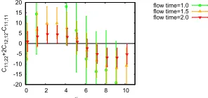
and correlation functions satisfy the following relation

C11;22(τ)+2C12;12(τ)−C11;11(τ)=0. (19)

In Fig.2we plot the left hand side of (19) as a function of the Euclidean time. The signal becomes better as we proceed the gradient flow. The linear combination is consistent with zero for all region within 1σ- 1.5σ.

-20 -15 -10 -5 0 5 10 15 20

0 2 4 6 8 10

C11;22 +2C 12;12 -C11;11 time flow time=1.0 flow time=1.5 flow time=2.0

Figure 2. A linear combination of correlation functions C11;22(τ)+2C12;12(τ)−C11;11(τ) as function of the

Euclidean time, which should vanish if the rotational symmetry is not broken. The flow timet/a2 _{=1.0 (green}

circle), 1.5 (orange up triangle), 2.0 (red down triangle).

4.3 Linear response relations

In this subsection we test linear response relations using the entropy density. The entropy density is expressed in three different ways. First it is written as (ϵ+p)/T by using the Maxwell’s relation and

the integrable condition for the entropy

s= ( ∂S ∂V ) T = ( ∂p ∂T ) V

=ϵ+p T = ⟨

T00+Tii⟩

T , (20)

which is given by the expectation value of one point function of the energy momentum tensor. On the other hand starting from a linear response of the pressure against a variation of the temper-ature the entropy density is given by a derivative of the energy momentum tensor

s= ( ∂p ∂T ) V

= ∂⟨Tii⟩

Substituting the statistical physics relation for the expectation value

⟨Tii⟩= 1

ZTr (

Tiie−H/T )

(22) we have the second expression in terms of the two point function of the energy momentum tensor

s= 1

T2⟨δHδTii⟩= 1 T2

∫

V3

d3_x(⟨_δT

00(τ, ⃗x)δTii(0)⟩)=T3C00;ii(τ). (23)

The last representation is given by using a linear response to the infinitesimal Lorentz boost

ϵ+p= ∂⟨T01⟩

∂v1

�� �� �_⃗v=0 =_T1

∫

V3

d3_x(⟨_{δT0i(τ, ⃗x)δT0i(0)}⟩)_=T4_{C0i;0i(τ). (24)}

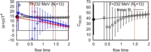
The correlation functions (23) and (24) are plotted as a function of the Euclidean time in the middle and right panel of Fig.1fori=2. According to the discussion given in subsection4.1three data at 5 ≤τ/a ≤7 are employed and fitted by a constant. The results are plotted in the left panel of Fig.3as a function of the flow time by blue down triangles (23) and red up triangles (24) for the entropy density divided by the temperature (ϵ+p)/T4. The contribution from the one point function

(20) is averaged over space-time and is plotted by black circles.

-10-5 0 5 10 15 20 25 30

0 0.5 1 1.5 2

(e+p)/T

4

flow time T=232 MeV (Nt=12)

0 10 20 30 40 50 60 70

0 0.5 1 1.5 2

C00;00

flow time T=232 MeV (Nt=12)

linear fit

Figure 3.The left panel is three different contributions (20) (black circles), (23) (blue down triangles) and (24) (red up triangles) to the entropy density plotted as functions of the flow time. ForC00;22 andC02;02we employ

three data at 5≤τ/a≤7 and fitted by a constant. The black and red dotted vertical lines indicate the linear window for the one and two point functions. The right panel isC00;00in (28) as a function of the flow time. Here

again three data at 5≤τ/a≤7 are taken and fitted by a constant.

After taking thet→0 limit (8) three contributions give the entropy density (ϵ+p)/T4. We adopt

the same strategy used in Refs. [10,11] to take the limit. The flowed operator (9) evaluated on the lattice behaves as follows as a function of the flow time

Tµν(t,a)=Tµν+t Sµν+Aµν

a2

t +t2Rµν, (25)

whereAµνappears due to the lattice artifact before taking the continuum limit.SµνandRµνare higher

dimensional irrelevant operator. What we find in our data is the linear window where the nonlinear contributionsa2_/tandt2 _{are negligible and data behaves linearly in the flow time. In the figure the} linear window is indicated by the black and red vertical dotted lines for the one point function (20) and two point correlators (23), (24). The data are fitted linearly intwithin the window to take the t→0 limit.

Substituting the statistical physics relation for the expectation value

⟨Tii⟩= 1

ZTr (

Tiie−H/T )

(22) we have the second expression in terms of the two point function of the energy momentum tensor

s= 1

T2⟨δHδTii⟩= 1 T2

∫

V3

d3_x(⟨_{δT00(τ, ⃗x)δTii(0)}⟩)_=T3_{C00;ii(τ). (23)}

The last representation is given by using a linear response to the infinitesimal Lorentz boost

ϵ+p= ∂⟨T01⟩

∂v1

�� �� �_⃗v=0=_T1

∫

V3

d3_x(⟨_{δT0i(τ, ⃗x)δT0i(0)}⟩)_=T4_{C0i;0i(τ). (24)}

The correlation functions (23) and (24) are plotted as a function of the Euclidean time in the middle and right panel of Fig.1fori=2. According to the discussion given in subsection4.1three data at 5 ≤τ/a ≤7 are employed and fitted by a constant. The results are plotted in the left panel of Fig.3as a function of the flow time by blue down triangles (23) and red up triangles (24) for the entropy density divided by the temperature (ϵ+p)/T4. The contribution from the one point function

(20) is averaged over space-time and is plotted by black circles.

-10-5 0 5 10 15 20 25 30

0 0.5 1 1.5 2

(e+p)/T

4

flow time T=232 MeV (Nt=12)

0 10 20 30 40 50 60 70

0 0.5 1 1.5 2

C00;00

flow time T=232 MeV (Nt=12)

linear fit

Figure 3.The left panel is three different contributions (20) (black circles), (23) (blue down triangles) and (24) (red up triangles) to the entropy density plotted as functions of the flow time. ForC00;22 andC02;02we employ

three data at 5≤ τ/a≤ 7 and fitted by a constant. The black and red dotted vertical lines indicate the linear window for the one and two point functions. The right panel isC00;00in (28) as a function of the flow time. Here

again three data at 5≤τ/a≤7 are taken and fitted by a constant.

After taking thet→0 limit (8) three contributions give the entropy density (ϵ+p)/T4. We adopt

the same strategy used in Refs. [10,11] to take the limit. The flowed operator (9) evaluated on the lattice behaves as follows as a function of the flow time

Tµν(t,a)=Tµν+t Sµν+Aµν

a2

t +t2Rµν, (25)

whereAµνappears due to the lattice artifact before taking the continuum limit.SµνandRµνare higher

dimensional irrelevant operator. What we find in our data is the linear window where the nonlinear contributionsa2_/tandt2_{are negligible and data behaves linearly in the flow time. In the figure the} linear window is indicated by the black and red vertical dotted lines for the one point function (20) and two point correlators (23), (24). The data are fitted linearly intwithin the window to take the t→0 limit.

The entropy density given by the linear fit is plotted by the corresponding filled symbols near the origin. Three different representations of the entropy density are consistent with each other within the statistical error. This indicates a success of the evaluation the energy-momentum tensor correlation functions.

4.4 Specific heat

The specific heat is given by a response of the energy against a variation of the temperature

cV = 1 V3

d⟨H⟩

dT . (26)

Inserting the statistical physics relation 1

V3⟨H⟩= 1 ZTr

(

T00(x)e−H/T) ₍₂₇₎

it is given in terms of the two point function of the energy momentum tensor

cV = 1 T2

∫

V3

d3_x(⟨_δT

00(τ, ⃗x)δT00(0)⟩)=T3C00;00(τ). (28)

The correlation function is plotted in the left panel of Fig.1. Here again data at 5≤τ/a≤7 are taken and fitted by a constant. The result are plotted in the right panel of Fig.3as a function of the flow time. As in the previous subsection we find the linear window indicated by the red vertical lines and perform the linear fit to take thet→0 limit. The resultant specific heat is plotted by the filled black circle at the origin, whose value iscV =38(27).

5 Conclusion

The two point correlation function of the renormalized energy-momentum tensor is calculated in Nf =2+1 QCD on lattice. On the lattice we confirmed the conservation law is realized apart from the point source. The spatial rotational symmetry is well shown within the statistical error.

The nonperturbative renormalization on lattice is done by applying the gradient flow to the gluon and quark fields and takinga→0 and thent→0 limits. Both limits are realized by making use of the linear window and applying the linear fit. This procedure is tested using the entropy density. Three difference representations are consistent with each other in thet →0 limit. Finally we calculate the specific heat by applying the method.

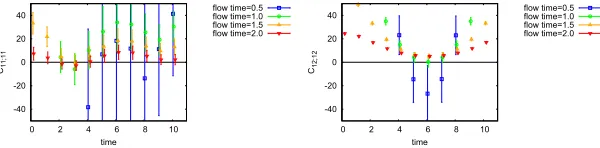
Future application shall be derivation of the bulk and shear viscosity using the corresponding two point correlation functions shown in Fig.4. We are also planning to calculate the correlation function

-40 -20 0 20 40

0 2 4 6 8 10

C11;11 time flow time=0.5 flow time=1.0 flow time=1.5 flow time=2.0 -40 -20 0 20 40

0 2 4 6 8 10

C12;12 time flow time=0.5 flow time=1.0 flow time=1.5 flow time=2.0

Figure 4.The bulk correlatorC11;11(τ) (left panel) and the shear correlatorC12;12(τ) (right panel) as a function of

the Euclidean time.

This work was in part supported by JSPS KAKENHI Grant Numbers JP25800148, JP26287040, JP26400244, JP26400251, JP15K05041, JP16H03982, and JP17K05442. This research used compu-tational resources of HA-PACS and COMA provided by the Interdisciplinary Compucompu-tational Science Program of Center for Computational Sciences at University of Tsukuba (No. 17a13), SR16000 and BG/Q by the Large Scale Simulation Program of High Energy Accelerator Research Organization (KEK) (Nos. 13/14-21, 14/15-23, 15/16-T06, 15/16-T-07, 15/16-25, 16/17-05), and Oakforest-PACS at JCAHPC through the HPCI System Research project (Project ID:hp170208). This work was in part based on Lattice QCD common code Bridge++[16].

References

[1] J. Adams et al. [STAR Collaboration], Nucl. Phys. A 757, 102 (2005) doi:10.1016/j.nuclphysa.2005.03.085 [nucl-ex/0501009].

[2] A. Nakamura and S. Sakai, Phys. Rev. Lett. 94, 072305 (2005)

doi:10.1103/PhysRevLett.94.072305 [hep-lat/0406009].

[3] H. B. Meyer, Phys. Rev. D 76, 101701 (2007) doi:10.1103/PhysRevD.76.101701 [arXiv:0704.1801 [hep-lat]].

[4] H. B. Meyer, Nucl. Phys. A 830, 641C (2009) doi:10.1016/j.nuclphysa.2009.09.053 [arXiv:0907.4095 [hep-lat]].

[5] M. Lüscher, J. High Energy Phys.1008, 071 (2010) Erratum: [J. High Energy Phys.1403, 092 (2014)] doi:10.1007/JHEP08(2010)071, 10.1007/JHEP03(2014)092 [arXiv:1006.4518 [hep-lat]].

[6] M. Lüscher and P. Weisz, J. High Energy Phys.1102, 051 (2011) doi:10.1007/JHEP02(2011)051 [arXiv:1101.0963 [hep-th]].

[7] M. Lüscher, J. High Energy Phys. 1304, 123 (2013) doi:10.1007/JHEP04(2013)123 [arXiv:1302.5246 [hep-lat]].

[8] H. Suzuki, Progr. Theor. Exp. Phys.2013, 083B03 (2013) Erratum: [Progr. Theor. Exp. Phys.

2015, 079201 (2015)] doi:10.1093/ptep/ptt059, 10.1093/ptep/ptv094 [arXiv:1304.0533 [hep-lat]].

[9] H. Makino and H. Suzuki, Progr. Theor. Exp. Phys. 2014, 063B02 (2014) Erratum: [Progr. Theor. Exp. Phys.2015, 079202 (2015)] doi:10.1093/ptep/ptu070, 10.1093/ptep/ptv095 [arXiv:1403.4772 [hep-lat]].

[10] Y. Taniguchi, S. Ejiri, R. Iwami, K. Kanaya, M. Kitazawa, H. Suzuki, T. Umeda and N. Wakabayashi, Phys. Rev. D 96, no. 1, 014509 (2017) doi:10.1103/PhysRevD.96.014509 [arXiv:1609.01417 [hep-lat]].

[11] Y. Taniguchi, K. Kanaya, H. Suzuki and T. Umeda, arXiv:1611.02411 [hep-lat]. Phys. Rev. D

95, no. 5, 054502 (2017) doi:10.1103/PhysRevD.95.054502 [arXiv:1611.02411 [hep-lat]]. [12] M. Kitazawa, T. Iritani, M. Asakawa and T. Hatsuda, arXiv:1708.01415 [hep-lat].

[13] T. Umeda et al. (WHOT-QCD Collaboration), Phys. Rev. D 85, 094508 (2012) doi:10.1103/PhysRevD.85.094508 [arXiv:1202.4719 [hep-lat]].

[14] T. Ishikawa et al. (JLQCD Collaboration), Phys. Rev. D 78, 011502 (2008) doi:10.1103/PhysRevD.78.011502 [arXiv:0704.1937 [hep-lat]].

[15] K. Kanayaet al.[WHOT-QCD Collaboration], arXiv:1710.10015 [hep-lat].