Plasmon mass scale and quantum fluctuations of classical fields
on a real time lattice
AleksiKurkela1,2,,TuomasLappi3,4, andJarkkoPeuron3, 1Theoretical Physics Department, CERN, Geneva, Switzerland
2Faculty of Science and Technology, University of Stavanger, 4036 Stavanger, Norway 3Department of Physics, P.O. Box 35, 40014 University of Jyväskylä, Finland
4Helsinki Institute of Physics, P.O. Box 64, 00014 University of Helsinki, Finland
Abstract.Classical real-time lattice simulations play an important role in understanding non-equilibrium phenomena in gauge theories and are used in particular to model the prethermal evolution of heavy- ion collisions. Above the Debye scale the classical Yang-Mills (CYM) theory can be matched smoothly to kinetic theory. First we study the limits of the quasiparticle picture of the CYM fields by determining the plasmon mass of the
system using 3 different methods. Then we argue that one needs a numerical calculation
of a system of classical gauge fields and small linearized fluctuations, which correspond to quantum fluctuations, in a way that keeps the separation between the two manifest. We demonstrate and test an implementation of an algorithm with the linearized fluctuation showing that the linearization indeed works and that the Gauss’s law is conserved.
1 Introduction
The Color Glass Condensate (CGC) [1] is an effective theory of QCD in the high energy (weak coupling) limit. In particular CGC predicts that gluon states of nonperturbatively high occupation numbers (>1/g2) are created in the initial stages of ultrarelativistic heavy ion collisions [2–4]. The highly occupied gluon states can be mathematically described using classical fields. The time-evolution of the classical system is given by the CYM equations
Dµ,Fµν
=0. (1)
We can neglect the fermion degrees of freedom because of the Pauli principle - the occupation number of the quark states can never exceed unity.
Due to the expansion of the system, the typical occupation numbers of the gluon states decrease over time. When they become perturbative, the system admits a kinetic theory [5] description. The kinetic theory evolution is followed by hydrodynamical evolution. Hydrodynamics, however, requires that the system is in local thermal equilibrium. Thus one of the most difficult problems in the field of ultrarelativistic heavy ion collisions is understanding the fast thermalization of the system [6]. Successful hydrodynamical description of the quark gluon plasma indicates, that thermalization
happens in a time of less than 1fm/c[7–10]. Recent studies have shown, that kinetic theory can be
matched smoothly to hydrodynamics, and the hydrodynamical regime can be reached within very short timescales using kinetic theory [11]. After subsequent hydrodynamical evolution the system expands and cools down, and finally freezes out.
In ”standard” lattice QCD (LQCD) one rotates to imaginary time and then tries to evaluate the path integral of the system. In this way one can compute equilibrium observables. We are interested in the time-evolution of the system in real time, and thus this standard approach is not applicable. However using classical approximation (which is valid in the highly occupied regime) one can do the time-evolution in a very straightforward manner. One has to simply take the classical lattice Lagrangian, and derive the classical equations of motion:
˙
Ui(x) = iEi(x)Ui(x) (2)
a2E˙i(x) = − ji
i,j(x)+i,−j(x)
ah. (3)
Here the plaquette variables are defined as
i,j(x)=Ui(x)Uj(x+ˆı)Ui†(x+ˆ)U†j(x) (4)
i,−j(x)=Ui(x)U†j(x+ıˆ−ˆ)Ui†(x−ˆ)Uj(x−ˆ) (5)
In numerical computations we use the SU(2) symmetry group. This simplifies the numerical work, and the results should be qualitatively similar to SU(3) [12–15].
2 Plasmon mass
From the kinetic theory point of view the interesting question is, whether we can understand these color fields in a quasiparticle picture [16]. We identify the field modes of the classical fields as plasmons. Based on a kinetic theory analysis [17] one expects the plasmon mass scale to evolve in time according tot−2/7power law when starting from an initial condition with a strongly overoccupied and UV finite isotropic distribution of gluons. In order to measure the plasmon mass we use three different methods.
2.1 Effective dispersion relation (DR)
The first method is to use an effective dispersion relation [2,18,19], defined as
ω2(k)=
E˙(k)2
|E(k)|2. (6)
In practice we extract the plasmon mass by doing a linear fit to the dispersion relation and extrapolating to zero momentum.
2.2 Uniform electric field method (UE)
The second method is a measurement which probes the response of the system to an external pertur-bation. We add a spatially uniform chromoelectric field [17] (corresponding to a perturbation with zero momentum) on top of the original field, and then we measure the oscillation frequency between electric and magnetic energies.
0.25
0.5
1
10
100
(t
Δ)
2/7
ω
pl2
/(
n
0Δ
2
)
tΔ
128
3n
0=0.1
n
0=0.5
n
0=1
n
0=2
n
0=3
n
0=5
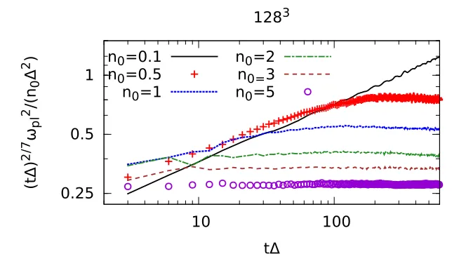
Figure 1: Time dependence of the plasmon mass obtained form our simulation, scaled by the inverse of the proposedt−2/7power law. We find that the late time behavior is compatible with this power law and that simulations with larger occupation numbers settle faster to this asymptotic behavior.
2.3 Perturbation theory, Hard Thermal Loop (HTL)
The third method is to use perturbation theory. In the Hard Thermal Loop (HTL) formalism the plasmon mass is given by
ω2pl =4 3g2Nc
d3k
(2π)3 f(k)
|k| , (7)
where f(k) is the quasiparticle distribution extracted from our simulation. The agreement between these methods is not clear a priori. The HTL formula assumes that the hard modes in the classical simulation behave like charged particles and give the dominant contribution to the plasmon mass. In this sense we are also testing this assumption here (However, the HTL method is probably the most commonly used way to measure plasmon mass in CYM thermalization studies [12,17,20]).
2.4 Results
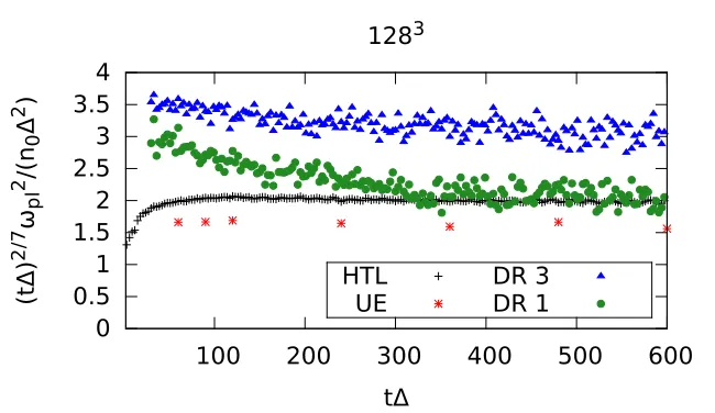
The results we obtain are shown in figures1and2. Figure1shows the time-evolution of the plasmon mass scale using the HTL method. The parametern0gives the typical occupation number used in the
0
0.5
1
1.5
2
2.5
3
3.5
4
100
200
300
400
500
600
(t
Δ)
2/7
ω
pl 2/(
n
0Δ
2
)
tΔ
128
3HTL
UE
DR 3
DR 1
Figure 2: Comparison of all three methods. Here DR 3 and DR 1 refer to the upper limits of the in the dimensionless momentum squared (k2
/∆2) used in the linear fit done to the dispersion relation.
3 Linearized fluctuations in CYM
Over last couple of years, the impact of fluctuations on the space-time evolution of an ultrarelativistic heavy ion collision has been studied. It has been shown that rapidly growing quantum fluctuations [22–26] may have a remarkable impact on the isotropization of a classical Yang-Mills system [27]. In these computations the fluctuations have been absorbed into the the classical background field. However, this kind of treatment of fluctuations is problematic because of two reasons. First one is that including fluctuations into the classical background is really justified only for the modes which grow large and become classical. The second problem is that one can not take continuum limit due to the fact that the fluctuation spectrum is highly UV-divergent. This means that on a fine enough lattice the UV tail of the spectrum entirely dominates the system.
Our aim is to improve the numerical treatment of these fluctuations by explicitly linearizing the fluctuation on top of the classical background and thus eliminating the backreaction from the fluctuations to the classical background [28]. This approach has two main applications in the future. The first one is simulating the boost invariance breaking quantum fluctuations and their contribution to thermalization. The second one is to use fluctuations to study linear response in classical Yang-Mills theory. For example one can study the dispersion relation and the damping rate of the plasma using fluctuations.
3.1 Equations of motion for fluctuations
Just like the background field, our fluctuation is split into two components: the fluctuation of the electric field and the fluctuation of the gauge field. Fluctuations will also have their own Gauss’ law.
3.1.1 Fluctuation of the electric field
We start by defining the required gauge transformation properties as those of an adjoint representation scalar field:
ai(x) → V(x)ai(x)V†(x) (8)
ei(x) → V(x)ei(x)V†(x). (9)
From these it follows thataihas to correspond to a variation of the link matrixUi(x) on the left:
Ui(x)bkg+fluct=eiai(x)Ui(x)≈Ui(x)+iai(x)Ui(x). (10)
The electric field fluctuation is introduced by adding a linear perturbation to the classical background. One simply replacesEiwithEi+ei. We choose to discretize the perturbation of the electric field by linearizing equation (3).
a2ei(t+dt)=a2ei(t)−dt ji
iai(x)i,j(x)+aj(x+ˆı→x)i,j(x)−i,j(x)ai(x+ˆ→x)
−i,j(x)aj(x)+ai(x)i,−j(x)−aj(x+ˆı−ˆ→x+ˆı→x)i,−j(x)
−i,−j(x)ai(x−ˆ→x)+i,−j(x)aj(x−ˆ→x)
ah
(11)
The parallel transported fluctuation from sitex+ˆıto sitexis denoted by
aj(x+ˆı→x)≡Ui(x)aj(x+ˆı)Ui†(x), (12)
and similarly for the fields parallel transported over two links
aj(x+ˆı−ˆ→x+ˆı→x)≡Ui(x)aj(x+ˆı−ˆ→x+ˆı)Ui†(x). (13)
In our notation there are two identical ways to write the most complicated terms involving parallel transport over two links.
3.1.2 Gauss’ law
The Gauss’ law for the fluctuations can be derived similarly as the equation of motion for the electric field fluctuation. One introduces both electric field fluctuations and gauge field fluctuations and discards the terms which are nonlinear in fluctuations. We get
c(x,t)=
i 1 a2
ei(x)−U†
i(x−ˆı)ei(x−ˆı)Ui(x−ˆı)+iU†i(x−ˆı)[ai(x−ˆı),Ei(x−ˆı)]Ui(x−ˆı)
=0.
3.1.3 Equation of motion for the fluctuation of the gauge field
The solution to this problem is to reverse engineer the correct update for the gauge field fluctuation using the Gauss’s law. For the background fields, the discretized Gauss’s law is conserved separately for the timesteps of links and electric fields. Demanding the same from the Gauss’s law of the fluctuation we obtain an update for the fluctuation of the gauge field (for SU(2))
ai(t+dt)=
−iEi,0iei⊥†0i
2TrEiEi +0ia ⊥
i†0i+dtei+ai(t), (14)
where the time like plaquette is denoted by0i=eiE
idt
. The notation⊥andrefers to the components ofaiandei, which are perpendicular or parallel to theEiin color space.
3.2 Numerical tests
We have also performed a couple of simple numerical tests to verify that our equations work as they should. The main things we want to verify are that the Gauss’s law is indeed conserved and that the linearization is correct. We have devised two tests. In the first one we test how well the different directions in Gauss’s law cancel each other. For the background fields we use the expression:
2 x Tr
i
Ei(x)−U†i(x−ˆı)Ei(x−ˆı)Ui(x−ˆı)
2
2 x,iTr
Ei(x)−U†
i(x−ˆı)Ei(x−ˆı)Ui(x−ˆı)
2 . (15)
And for the fluctuations we have:
2 xTr
i
ei(x)−U†
i(x−ˆı)ei(x−ˆı)Ui(x−ˆı)+iUi†(x−ˆı)[ai(x−ˆı),Ei(x−ˆı)]Ui(x−ˆı)
2
2 x,iTr
ei(x)−U†
i(x−ˆı)ei(x−ˆı)Ui(x−ˆı)+iUi†(x−ˆı)[ai(x−ˆı),Ei(x−ˆı)]Ui(x−ˆı)
2 . (16)
Here the numenator is simply the Gauss’s law squared integrated over the whole lattice. The denomina-tor is the sum of squares summed over the whole lattice. We test this using single and double precision numbers. If there is a deviation between the two, then the differences in accuracy are explained by variations in the machine precision. However, if these two will converge to same value, it means that there is a greater source of error than machine precision. Results are shown in figure3a. We observe that the Gauss’s law is conserved much better for double precision numbers than single precision numbers, indicating that the difference is caused by finite machine precision. We also perform a random gauge transformation on every time step and fix Coulomb gauge on every tenth timestep to verify gauge invariance numerically.
The second test probes whether the linearization works correctly. We do two simulations using two different configurations. HereE is the background electric field andeis the fluctuation of the electric field. The scale of the fluctuation is set by a multiplicative parameter.In the first simulation we initiate the simulation by absorbing bothEandeto the classical background and evolve this in time. The result will be labeled asEB. At the initial time we haveEB=E+e. In another simulation we use two dynamical fields, the background field and the fluctuation field, which are evolved separately with their own solvers (The background fields appear in the equations of motion of the fluctuations of course.). We denote these fields byEAandeA. InitiallyEA=EandeA =e. After evolving these two simulations in time, we measure TrE˙B−E˙A−e˙A
2
The solution to this problem is to reverse engineer the correct update for the gauge field fluctuation using the Gauss’s law. For the background fields, the discretized Gauss’s law is conserved separately for the timesteps of links and electric fields. Demanding the same from the Gauss’s law of the fluctuation we obtain an update for the fluctuation of the gauge field (for SU(2))
ai(t+dt)=
−iEi,0iei⊥†0i
2TrEiEi +0ia ⊥
i †0i+dtei+ai(t), (14)
where the time like plaquette is denoted by0i=eiE
idt
. The notation⊥andrefers to the components ofaiandei, which are perpendicular or parallel to theEiin color space.
3.2 Numerical tests
We have also performed a couple of simple numerical tests to verify that our equations work as they should. The main things we want to verify are that the Gauss’s law is indeed conserved and that the linearization is correct. We have devised two tests. In the first one we test how well the different directions in Gauss’s law cancel each other. For the background fields we use the expression:
2 x Tr i
Ei(x)−U†i(x−ˆı)Ei(x−ˆı)Ui(x−ˆı)
2
2 x,iTr
Ei(x)−U†
i(x−ˆı)Ei(x−ˆı)Ui(x−ˆı)
2 . (15)
And for the fluctuations we have:
2 x Tr i
ei(x)−U†
i(x−ˆı)ei(x−ˆı)Ui(x−ˆı)+iU†i(x−ˆı)[ai(x−ˆı),Ei(x−ˆı)]Ui(x−ˆı)
2
2 x,iTr
ei(x)−U†
i(x−ˆı)ei(x−ˆı)Ui(x−ˆı)+iUi†(x−ˆı)[ai(x−ˆı),Ei(x−ˆı)]Ui(x−ˆı)
2 . (16)
Here the numenator is simply the Gauss’s law squared integrated over the whole lattice. The denomina-tor is the sum of squares summed over the whole lattice. We test this using single and double precision numbers. If there is a deviation between the two, then the differences in accuracy are explained by variations in the machine precision. However, if these two will converge to same value, it means that there is a greater source of error than machine precision. Results are shown in figure3a. We observe that the Gauss’s law is conserved much better for double precision numbers than single precision numbers, indicating that the difference is caused by finite machine precision. We also perform a random gauge transformation on every time step and fix Coulomb gauge on every tenth timestep to verify gauge invariance numerically.
The second test probes whether the linearization works correctly. We do two simulations using two different configurations. HereEis the background electric field andeis the fluctuation of the electric field. The scale of the fluctuation is set by a multiplicative parameter.In the first simulation we initiate the simulation by absorbing bothEandeto the classical background and evolve this in time. The result will be labeled asEB. At the initial time we haveEB =E+e. In another simulation we use two dynamical fields, the background field and the fluctuation field, which are evolved separately with their own solvers (The background fields appear in the equations of motion of the fluctuations of course.). We denote these fields byEAandeA. InitiallyEA=EandeA =e. After evolving these two simulations in time, we measure TrE˙B−E˙A−e˙A
2
,or alternatively TrAB−AA−aA2for the
(a) Violation of the Gauss’s law of the fluctuations as a function of time with single and double precision numbers. We have performed a random gauge transfor-mation on every time step and fixed Coulomb gauge on every tenth timestep.
1e-14 1e-12 1e-10 1e-08 1e-06 0.0001 0.01 1 100 10000
0.0001 0.001 0.01 0.1 1 ε
Σx,iTr(d(EBi-EAi-ei)/dt)2 Σx,iTr(ABi-AAi-ai)2
(b) Test of the decomposition of the field in the back-ground field and fluctuation after some finite time. The straigth lines are fits of the formax4demonstrating the
correct power law.
gauge fields. If the linearization is done correctly, linear term inin the difference should cancel. Thus the traces of the squares should scale as4.The results are shown in figure3b, where we observe the correct scaling.
4 Conclusions
We have studied the plasmon mass in pure glue QCD using three different methods: the effective dispersion relation, the uniform electric field method and perturbative formula relating the quasiparticle spectrum to the plasmon mass. It turns out that HTL and UE methods can be brought into rough agreement, but the DR method agrees with other methods within a factor of two. The conclusion from the agreement between the UE and HTL methods is that the kinetic theory description using weakly interacting quasiparticles seems to be valid way to understand overoccupied system of classical gauge fields, even quantitatively.
We have also developed a way to simulate dynamical fluctuations on top of classical background. We have derived, implemented and tested linearized equations for fluctuations in classical Yang-Mills theory on the lattice, and verified that they conserve the Gauss’s law.
Our future goals are to study plasmon mass in 2 dimensional systems, mimicking 2+1 dimensional boost invariant systems, which arise in the weak coupling framework in ultrarelativistic heavy ion collisions. We also have plans to apply fluctuations in our future studies. A straightforward application we are working on is to study the dispersion relation of weakly coupled plasma by using fluctuations to study linear response in CYM.
Acknowledgements
References
[1] E. Iancu, R. Venugopalan (2003),hep-ph/0303204 [2] T. Lappi, Phys. Rev.C67, 054903 (2003),hep-ph/0303076
[3] T. Lappi, L. McLerran, Nucl. Phys.A772, 200 (2006),hep-ph/0602189
[4] F. Gelis, E. Iancu, J. Jalilian-Marian, R. Venugopalan, Ann. Rev. Nucl. Part. Sci.60, 463 (2010), 1002.0333
[5] P.B. Arnold, G.D. Moore, L.G. Yaffe, JHEP01, 030 (2003),hep-ph/0209353 [6] J. Berges, J.P. Blaizot, F. Gelis, J. Phys.G39, 085115 (2012),1203.2042 [7] K. Aamodt et al. (ALICE), Phys. Rev. Lett.105, 252302 (2010),1011.3914 [8] P. Huovinen (2003),nucl-th/0305064
[9] P. Kolb, P. Huovinen, U.W. Heinz, H. Heiselberg, Phys. Lett. B500, 232 (2001), hep-ph/0012137
[10] T. Hirano, P. Huovinen, Y. Nara, Phys. Rev.C83, 021902 (2011),1010.6222 [11] A. Kurkela, Y. Zhu, Phys. Rev. Lett.115, 182301 (2015),1506.06647
[12] J. Berges, M. Mace, S. Schlichting, Phys. Rev. Lett.118, 192005 (2017),1703.00697 [13] A. Ipp, A. Rebhan, M. Strickland, Phys.Rev.D84, 056003 (2011),1012.0298
[14] J. Berges, D. Gelfand, S. Scheffler, D. Sexty, Phys. Lett.B677, 210 (2009),0812.3859 [15] A. Krasnitz, Y. Nara, R. Venugopalan, Phys. Rev. Lett.87, 192302 (2001),hep-ph/0108092 [16] T. Lappi, J. Peuron, Phys. Rev.D95, 014025 (2017),1610.03711
[17] A. Kurkela, G.D. Moore, Phys. Rev.D86, 056008 (2012),1207.1663
[18] A. Krasnitz, R. Venugopalan, Phys. Rev. Lett.86, 1717 (2001),hep-ph/0007108 [19] J. Berges, S. Schlichting, D. Sexty, Phys. Rev.D86, 074006 (2012),1203.4646 [20] J. Berges, K. Boguslavski, S. Schlichting, R. Venugopalan (2013),1311.3005 [21] M. Gyulassy, L. McLerran, Nucl. Phys.A750, 30 (2005),nucl-th/0405013
[22] K. Fukushima, F. Gelis, L. McLerran, Nucl. Phys.A786, 107 (2007),hep-ph/0610416 [23] K. Dusling, T. Epelbaum, F. Gelis, R. Venugopalan, Nucl. Phys.A850, 69 (2011),1009.4363 [24] T. Epelbaum, F. Gelis, Nucl. Phys.A872, 210 (2011),1107.0668
[25] K. Dusling, R. Venugopalan, Phys. Rev. Lett.108, 262001 (2012),1201.2658 [26] T. Epelbaum, F. Gelis, Phys. Rev.D88, 085015 (2013),1307.1765