Likelihoods and Simulation Methods for a Class of
Nonneutral Population Genetics Models
Peter Donnelly,* Magnus Nordborg
†,1and Paul Joyce
‡*Department of Statistics, University of Oxford, Oxford OX1 3TG, United Kingdom,†Department of Genetics, Lund University, Lund 223 62, Sweden and‡Department of Mathematics and Division of Statistics, University of Idaho, Moscow, Idaho 83844-1104
Manuscript received March 22, 1999 Accepted for publication July 12, 2001
ABSTRACT
Methods for simulating samples and sample statistics, under mutation-selection-drift equilibrium for a class of nonneutral population genetics models, and for evaluating the likelihood surface, in selection and mutation parameters, are developed and applied for observed data. The methods apply to large populations in settings in which selection is weak, in the sense that selection intensities, like mutation rates, are of the order of the inverse of the population size. General diploid selection is allowed, but the approach is currently restricted to models, such as the infinite alleles model and certain K-models, in which the type of a mutant allele does not depend on the type of its progenitor allele. The simulation methods have considerable advantages over available alternatives. No other methods currently seem practicable for approximating likelihood surfaces.
T
HE neutral theory provides a natural null hypothe- tensive. On the other hand, our simulation algorithmsappear to have advantages over available alternatives sis in many evolutionary contexts, and the behavior
of neutral models is now rather well understood. On (all of which are also computationally intensive). While
the methods require substantial computational effort, the other hand, any assessment of the forces generating
and maintaining genetic diversity also requires an un- they remain practicable.
Throughout, we use “frequency” to refer to relative derstanding of the behavior of a range of nonneutral
models. More formally, at least in the context of data frequencies.
at a single locus, the development of efficient tests of neutrality against particular selective alternatives, and
THEORETICAL BACKGROUND
efficient inference for mutation and selection parame-ters, requires methods for evaluating or approximating
We now describe the class of evolutionary models to likelihood surfaces under the selective models of
in-which our results apply. For concreteness we first set
terest. the discussion in the context of the Wright-Fisher model
In this article, we develop and apply methods for the for the evolution of a panmictic population of constant
simulation of samples from nonneutral models and for size
Ndiploid individuals. WriteEfor the collection of
approximating the distribution of summary statistics of possible alleles in the population. We assume that the
sample diversity. We also give a method for approximat- probability that any particular allele in a given
genera-ing the likelihood function, in the evolutionary parame- tion will be a mutant copy of its progenitor allele isu,
ters, for observed data. This is applied to two data sets, regardless of the type of the progenitor allele. We
fur-one from Drosophila where purifying selection appears ther assume throughout that when a mutation occurs
to be operating, and one from Borrelia burgdorferi, the the (random) type of the mutant gene does not depend
cause of Lyme disease, in which there appears to be on the type of the progenitor allele. This assumption
balancing selection. While our approach allows general applies, for example, to an infinite-alleles model and
diploid selection, it is currently applicable only to mod- to someK-allele models. It does not hold for stepwise
els for mutation in which the type of mutant does not mutation models nor for most models that aim to model
depend on the type of parent, such as the infinite-alleles DNA sequences directly, including the infinite-sites
model. model. If a mutation occurs, we writefor the
distribu-The methods described here are computationally in- tion of the type of the mutant allele.
Write wN(Ai, Aj) (⫽ wN(Aj, Ai)) for the fitness of an
individual with genotype (Ai,Aj). In forming the next
Corresponding author:Peter Donnelly, Department of Statistics, Uni- generation, 2N pairs of genes are first selected from versity of Oxford, 1 S. Parks Rd., Oxford OX1 3TG, United Kingdom.
the current generation. These choices are independent, E-mail: [email protected]
and the chance that a particular pair (Ai,Aj) is selected 1Present address:Department of Biological Sciences, University of
Southern California, Los Angeles, CA 90089-1340. at each choice is proportional towN(Ai,Aj). Next, one
of the genes within each pair is chosen uniformly. With have the same fitness. The normalizing constant,C, will
probability 1⫺ua nonmutant copy of that gene will be in general depend on the mutation parameters and
included in the next generation, while with probabilityu and the fitness function(·, ·). (Note that the original
a mutation will occur, in which case the type of the fitness function still appears in the exponential factor
mutant will be chosen according to the distribution on the right of Equation 2.)
. This selection and possibly mutation from within a It turns out that sampling distributions for models
chosen pair is independent between pairs. with selection may be written in terms of properties of
Our results actually apply to the usual diffusion ap- the analogous neutral model, and our purpose here is
proximation of this model, which arises for a large, to explore various statistical consequences of this fact.
panmictic population of constant size N, in which the For the configuration Xn of a sample of size n, write
forces of genetic drift, mutation, and selection are com- LS(Xn) for the probability of obtaining such a sample at
parable in size. As is usual, we scale the mutation and equilibrium in the diffusion model described above.
selection parameters and write ⫽4Nuand(Ai,Aj)⫽ Further, we writeLN(Xn) for the probability of obtaining
2N(wN(Ai,Aj)⫺1). Note that exactly the same diffusion such a sample in the diffusion model with the same
approximation applies to a wide range of population mutation structure but in which all genotypes have equal
models and hence our results relate more generally fitness.Joyce(1994) established that
than to the Wright-Fisher model.
LS(Xn)⫽LN(Xn)⺕N(g(X)|Xn). (4)
Our concern is with distributions that arise in the diffusion approximation of populations at (stochastic)
The second factor on the right of (4) represents the equilibrium under the forces of drift, mutation, and
expected value of the functiong(X), where the distribu-selection. Specifically we relate properties of these
distri-tion ofXis the conditional distribution, under neutral-butions in the general model to those that arise under
ity, of the composition of the population given that a neutrality, which can be thought of as the special case in
sample from it has distributionXn.
which(Ai,Aj)⫽ 0 for all possible genotypes (Ai,Aj).
The importance of the relation (4) is that it relates The genetic composition of a population can be
de-sampling distributions under selection to quantities that scribed by listing the alleles present in the population
arise in neutral models. For the class of models we are
together with their frequencies. We useXto denote a
considering, the probabilitiesLN(Xn) are known
explic-generic population and think of this as a list {(A1, x1),
itly. Under neutrality, the conditional distribution of (A2,x2), . . . } in which the alleles present areA1,A2, . . .
the composition of the population given the sample is with respective frequencies x1, x2, . . . (so that xi ⱖ 0,
also known for the class of models considered here. As i⫽1, 2, . . . , andx1⫹x2⫹. . .⫽1). One can think of
a consequence, the second factor in (4) can also be the diffusion approximation as describing the evolution
evaluated, perhaps by simulation. of a hypothetical infinite population whose genetic
com-position may be described in exactly this way. In the same way we can describe the genetic composition of a
SPECIFIC MODELS
sample Xn from the population as a list of the alleles
present in the sample together with their (relative) fre- We now consider some concrete examples of models
quencies in the sample. to which our analysis applies.
We denote the mean fitness of a population X by K-allele models:Consider a model withK alleles, so
* (X), thatE⫽{A
1,A2, . . . ,AK}. Assume that the scaled
muta-tion rate for each allele is and that a mutant allele
*(X)⫽
兺
i,j
(Ai,Aj)xixj (1)
will beAiwith probabilityi,i⫽1, . . . ,K, independently
for each mutant. As above, we write (Ai, Aj) for the
(Ethier andKurtz 1994). In what follows it is often
scaled fitness of the genotype (Ai,Aj).
helpful to think of the mean fitness as a function ofX,
In this setting, the sampling distribution under neu-the composition of neu-the population. A furneu-ther function
trality is of the population composition is destined to play a
central role in the sequel. Define
LN(Xn)⫽
n!(1)(n1)· · · (K)(nK)
n1! · · ·nK!()(n)
, (5)
g(X)⫽C⫺1exp(*(X)). (2)
HereCis chosen so that⺕N(g(X))⫽1,i.e., in which we have written ni ⫽ nxi for the number of
copies of allele Ai in the sample and the notation z(n)
C ⫽⺕N(exp(*(X))), (3)
for the rising factorialz(n)⫽ z(z⫹1) · · · (z ⫹n⫺1).
Further, under neutrality, the conditional distribution where exp denotes the exponential function, and the
of the population given the sample Xn is a Dirichlet
expectation, ⺕N, is taken over the distribution of the
distribution with parameters (1 ⫹ n1, 2 ⫹ n2, . . . ,
population composition,X, for the neutral model with
ber of copies of allelei in the sample. It remains to f(x1. . . ,xK)⫽
⌫(
兺
Ki⫽1i⫹ ni)
兿
Ki⫽1⌫(i⫹ ni)
兿
ki⫽1
xi⫹ni⫺1
i , (6) describe the way in which the total frequency W of
“new” alleles, those that occur in the population but not
for Rxi ⫽ 1. Equations 5 and 6 follow, for example, the sample, is broken up among these various alleles. In
fromWright’s (1949) characterization of the stationary fact, the proportion of new alleles of the various types distribution for population allele frequencies as Dirich- has a GEM distribution, independent ofX1,X2, . . . ,Xk,
let and elementary properties of multinomial samples W.Thus, labeling these new allelesk⫹ 1,k⫹2, . . . ,
from the Dirichlet distribution (e.g., Bernardo and the population frequencies can be written
Smith1994).
(X1, . . . ,Xk,Xk⫹1,Xk⫹2, . . .), (8)
A special case of this model was used byHartland
Sawyer (1991) to estimate the amount of selection whereX
k⫹i ⫽WZi,i⫽ 1, 2, . . . , and (Z1,Z2, . . .) has a
needed to explain amino acid replacement polymor- GEM distribution with parameter, independent ofX
1,
phism. In their modelK⫽4 with the alleles representing X
2, . . . , Xk, W.For further background see Donnelly
the four nucleotides. They considered a genic selection andTavare´ (1987) orEwens(1990).
regime in which one of the nucleotides was favored, say Various selective schemes may be of interest in the
A. Then(A,A)⫽2,(A,C)⫽ (A,G)⫽ (A,T)⫽ infinite-alleles context. We describe two explicitly and
, and(x,y)⫽0 for all other genotypes. consider them in further detail in subsequent sections.
Infinite alleles:For infinite-alleles models with scaled The first is heterozygote advantage, in which all
het-mutation rate, the neutral sampling formula LN(Xn) erozygotes have equal fitness and all homozygotes have
is given by the Ewens sampling formula (Ewens1972), equal fitness that is lower than that of the heterozygotes.
In our notation LN(Xn)⫽
n!
(n)
兿
Nj⫽1
冢
j
冣
aj 1
aj!
, (7)
(x,y)⫽
冦
⫺0 ififxx⬆⫽yy. in whichajis the number of alleles withjrepresentativesGroteandSpeed(2001) consider this model in some in the sample.
detail. Under neutrality, the allele frequencies, (X1,X2, . . . ),
A second set of selective schemes arises when the in the population follow the so-called GEM distribution
collection of possible alleles is broken up into classes. with parameter,
The simplest example arises when there are two classes,
X1 ⫽V1 which we call neutral and deleterious. WriteNandD
for the neutral and deleterious classes, respectively. The X2 ⫽(1⫺ V1)V2
fitnesses are then .
.
. (x,y)⫽
冦
0 ifx,y僆N
⫺12 ifx僆 N,y僆Dor x僆 D,y僆N
⫺22 ifx,y僆D. Xi ⫽(1⫺ V1)(1⫺ V2) . . . (1⫺Vi⫺1)Vi
There are obvious generalizations to schemes with more
than two selective classes. See, for example,Joyceand
. .
. Tavare´(1995) andJoyce(1995).
in which theViare independent and identically
distrib-APPLICATIONS
uted random variables with probability density
The theoretical results presented above lead naturally
f(v)⫽ (1⫺ v)⫺1, 0ⱕvⱕ1
to several computational applications. In this section, three such applications are described in general terms:
(see, for example,DonnellyandTavare´ 1987).
To apply (4) we need the conditional distribution of they are illustrated in two specific genetic models in the
following two sections. The software used is available the population given the configuration,Xn, in the
sam-ple. Suppose there arek alleles in the sample, which from the authors.
Simulating samples:In view of the relation (4), sam-we label 1, 2, . . . ,k. These alleles must belong to the
population, and we writeX1,X2, . . . ,Xkfor their popula- ples from the nonneutral model can be obtained by
rejection sampling. The idea is to generate neutral sam-tion frequencies. There will also be (an infinite number
of) alleles in the population that do not appear in the ples,Xn, and to “accept” or “reject” each one according
to the value of⺕N(g(X)|Xn). The collection of accepted
sample. WriteWfor the total frequency in the
popula-tion of these alleles. Condipopula-tional on the sample frequen- samples will then be an independent sequence of
sam-ples from the appropriate model with selection. For cies, the distribution of (X1,X2, . . . ,Xk,W) is Dirichlet
called acceptance sampling), see, for example,Ripley Step 2 of the rejection algorithm requires simulation
(1987). from the conditional distribution of the population,X,
It is convenient to introduce a notation for the fitness given the sample,Xn. ForK-allele models, the required
of the fittest genotype. Definemaxto be the maximum, conditional distribution is the Dirichlet distribution (6).
across all possible genotypes, of the scaled selection For the infinite-alleles model, it is given by Equation 8.
coefficients: There are also several ways to simulate X given Xn,
i.e., to carry out step 2 of the rejection algorithm. As
max⫽ max
兵
(x,y), x,y僆E其
.we described in the previous section, the analytic form (under neutrality) of the population distribution condi-For example, in both the infinite alleles models
de-tional on the sample is known explicitly for the models
scribed above, max ⫽ 0. Samples from the models we
we are considering. We thus generate Xdirectly from
are considering may be generated as follows.
this distribution.
Algorithm1: The rejection method for simulating non- SamplesXn, which arise from these simulations,
con-neutral samples: tain information about the allele frequencies and the
labels of the alleles. Thus, for example, in a two-class
1. Simulate a sample,Xn, from the neutral model.
model, it will be known which alleles in the sample
2. Simulate a population composition,X, conditional onXn.
belong to which class. This division of alleles into classes
3. Simulate U, an independent uniform random variate on
will not be known for many actual data sets. Simulation [0, 1].
of data of this sort may be achieved simply by ignoring 4. If Uⱕ exp(*(X)⫺max), reportXnas a sample from
the allele labels in the samples simulated as above.
the nonneutral model. Otherwise return to step1.
The scheme above applies to any of the nonneutral
The efficiency of this algorithm depends mostly on how models within the class we are considering. Special
fea-often samples are accepted. It is clear that, for some tures of particular such models may lead to other
simula-models with very strong selection, the rejection scheme tion schemes for those models. For example,
Wat-may be too slow to be practical. terson (1987) used an urn scheme to generate data
Several methods for simulating neutral samples (i.e., under the two-class model with genic selection. Li
for carrying out step 1) exist. For the neutral models (1993) used a related rejection-based scheme for this
we are considering, the following algorithm, similar to model.
the one used by Li(1993), is convenient. Estimating the distribution of sample statistics: A
common reason for simulating samples is to estimate
Algorithm 2: The urn scheme for generating neutral
the distribution of some sample statistic. Two related samples:
approaches, each exploiting (4), are available for this
1. Start with an urn containing a single black ball of mass. problem in the context of the nonneutral models we
2. At each stage, independently of the past, draw a ball from are considering. The first is simply to use the rejection
the urn with probability proportional to its mass. method just described to simulate a large number,m
a. If the black ball is chosen, return it to the urn together say, of samples from the appropriate model, to evaluate
with a ball of unit mass whose type is chosen (indepen- the statistic of interest for each of the simulated samples,
dently of everything else) according to the distribution and to approximate its distribution by the histogram of
on E. simulated values.
b. If a ball other than the black ball is chosen, return it The second approach is based on importance
sam-to the urn sam-together with an additional ball of unit mass pling. (For background, see Ripley 1987.) Write f(·)
whose type is identical to that of the chosen ball. for the sample statistic of interest.
3. Stop when the urn contains n balls other than the black
Algorithm3:Importance-sampling scheme for estimating ball.
the distribution of a sample statistic: The collection of types of balls, other than the black
ball, in the urn has the distribution, LN(Xn), of the 1. Simulate a collection of samples from the neutral model,
configuration of a sample of sizenfrom the appropriate X(i)
n ,i ⫽1, 2, . . . ,M.
neutral model (Hoppe1984;Donnelly1986). 2. For the ith such sample, X(i)
n ,simulate, under neutrality,
In the case of the K-allele models described above, a valueX(i)for the population composition given that the
the balls added to the urn can simply be labeled from sample configuration isX(i)
n .Evaluatei⫽exp(*(X(i))).
the integers 1, 2, . . . ,K. One convenient method for 3. Create a histogram that assigns probabilityi/RM
j⫽1jto the
dealing with infinite-alleles models is to label each suc- ith observed value of the sample statistic f(X(i) n ).
cessive allele introduced by choosing an independent
The resulting histogram estimates the distribution of uniform random variable from [0, 1]. Another
possibil-f(Xn), whereXnis a sample from the nonneutral model.
ity is to use the integers 1, 2, 3, . . . , successively, as the
moment (under the nonneutral model) of the statistic, have extremely low mean fitness and with low probabil-ity have high fitness (consider the probabilprobabil-ity of observ-is just
ing a functioning mitochondrion if mutation were the only factor governing molecular evolution!). The
distri-兺
M i⫽1i
兺
Mj⫽1j
f(X(i)
n )k. (9)
bution of exp(*(X)) is thus extremely skewed, and
its expectation is difficult to estimate. Note that the In particular, the mean value of the statistic is estimated
distribution of exp(*(X)) conditional on the observed
from (9) withk⫽1.
sample is usually much better behaved, because the The first two steps in the importance sampling method
selective scheme will typically be chosen to fit the sam-just described are carried out exactly as for the rejection
ple. We return to these issues in the examples below.
scheme above. Note that, since theXnandXare drawn
from the relevant neutral distribution, they can be
re-used for all selection schemes of interest (e.g., for differ- PURIFYING SELECTION
ent values of the parameters describing the strength of
As described above, deleterious mutation can be mod-selection). This improves the efficiency of the method
eled in the infinite-alleles framework by letting the col-considerably.
lection of all possible alleles (which we label as points The idea of the importance sampling scheme is that
in [0, 1]) be divided into the class of wild-type alleles,
eachsimulated neutral sample is used in estimating the
N ⫽ [0, a), and the class of deleterious alleles, D⫽
distribution of the statistic, but the neutral samples are
[a, 1]. Thus the scaled deleterious mutation rate is (1⫺ given different weights—those that are more likely
un-a), and the rate of back mutationa, so ashould be der the selection scheme of interest are given relatively
close to zero for this model to be at all reasonable. higher weights than those that are unlikely. In contrast,
We use the common fitness parameterization 1, 1⫺
the rejection scheme makes a simple (randomized)
sh, and 1 ⫺s for the homozygous wild type,
heterozy-“yes/no” decision about whether to include or exclude
gote, and homozygote deleterious, respectively. The
ap-each neutral sample. As discussed in theappendix, the
propriately scaled fitness coefficients are thus 12 ⫽
importance sampling scheme is more efficient.
2Nsh and 22⫽ 2Ns. Note that if h is small (recessive
Likelihood analysis:It is also possible to carry out
full-mutations) and the mutation rate small relative to the likelihood analyses on the basis of (4). The likelihood
strength of selection, the mean equilibrium frequency for a sampleXninvolves the following three quantities:
of deleterious alleles will also be small and close to the
deterministic approximation/212(Haldane1927).
1. LN(Xn), the likelihood of the sample under neutrality.
Likelihood for simulated samples: We first demon-2. ⺕N(exp(*(X))|Xn).
strate the calculation of a likelihood surface on samples
3. The normalizing constant C ⫽ ⺕N(exp(*(X))),
simulated with known parameters usingAlgorithm 1.
Fig-where the expectation is taken over the distribution
ures 1 and 2 show two such examples. Furthermore, it of the unconditional population composition.
seems that there is enough information in samples
un-Multiplying the first and second quantities, and dividing der this model to obtain reasonable estimates of both
by the third, gives the likelihood under the nonneutral and22.
model. These examples also illustrate some of the predicted
Since, as we have seen, the sampling distribution is problems with the methods. First, both samples
re-known for the neutral models that we are considering, quired on the order of 104 rejections, which is not a
the first quantity can be calculated numerically. For problem when generating only a few samples, but can
example, for theK-allele model it is given by (5) and make simulating large numbers of samples prohibitively
for the infinite-alleles model it is the Ewens sampling time consuming. Second, the surfaces have “ridges”
formula (7). along the22-axis and look jagged along the-axis. The
The second quantity is estimated as described for the ridges are caused by the fact that we (as described in
second step in the importance sampling method. the previous section) reuse the population compositions
The third quantity can be estimated by generating a generated for a given for all selection values. The
large number of (unconditional) population composi- values along the22-axis are thus completely correlated.
tions,X, calculating exp(*(X)) for each of them, and This would not be a problem if the values along the
taking the average. We note that, as before, it is possible -axis were well estimated, but they are clearly not. It
to use the same set of simulatedXfor several different turns out that the problem here lies in the estimation of
selection schemes. the constantC, which is very difficult under this model.
Although in principle straightforward, it turns out Fortunately, there is also an easy alternative for this
that this last step can sometimes be computationally model, because exp(*(X)) depends only on the
fre-extremely difficult. The reason for this is simple enough: quency of deleterious alleles, not the entire
composi-if selection is strong, then populations that have evolved tion. Under neutrality, it can be shown, for example,
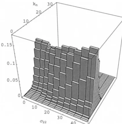
Figure2.—Likelihood surface inand22for sample of sizen⫽100 simulated under the deleterious-mutation model with ⫽ 4, a ⫽ 10⫺3, h ⫽ 0.2, and 22 ⫽ 10. Haldane’s Figure1.—Likelihood surface in and22for sample of approximation is not valid in this case because the equilibrium sizen⫽100 simulated under the deleterious-mutation model frequency of deleterious alleles is not small; the simulated with ⫽ 1, a ⫽ 10⫺3, h ⫽ 0.2, and 22 ⫽ 100. Haldane’s
sample, which required 21,420 rejections, contained 64 copies approximation predicts the equilibrium frequency of deleteri- of a single wild-type allele and 8 distinct deleterious alleles in ous alleles, 2.5%; the simulated sample, which required 27,789 frequencies 13, 7, 5, 5, 2, 2, 1, 1. The surface has a maximum rejections, contained 2 different alleles, 3 deleterious, and 97 at ⫽3.5 and22⫽15 and was constructed using the same wild-type. The surface has a maximum at ⫽0.5 and 22⫽ number of repetitions as Figure 1.
40, parameters for which Haldane’s equilibrium is 3.1%. In constructing the surface, 107repetitions pervalue were used to estimateCand 105to estimate⺕
N(exp(*(X))|Xn).
different alleles, 8 of which were singletons and 1 of which appeared at a frequency close to 60%. Under the neutral infinite-alleles model, ˆ, the
maximum-likeli-(1⫺a) anda, respectively, between the two alleles,
that the frequency of deleterious alleles in the popula- hood estimate ofisⵑ5. The expected sample
homozy-tion under the present mutahomozy-tion scheme is-distributed gosity,⺕(Fn), for ⫽5 is 0.17. The observedFnis much
with parameters(1⫺a) anda, and it is thus possible higher, 0.37, and neutrality is rejected by the
Ewens-to calculateCthrough numerical integration. Figure 9 Watterson test (Watterson1978), a plausible
alterna-in the followalterna-ing section illustrates how much this can tive hypothesis being that all alleles but the most
com-improve the estimation. mon one are deleterious.
Xdh in Drosophila pseudoobscura: We now turn to a Assuming ⫽5,a⫽0.01, andh⫽0.2, we used Algo-real data set, namely that ofKeithet al.(1985). Using rithm 3to approximate the distributions ofkn,Fn, and the
sequential electrophoresis, they observed the following sample frequency of deleterious alleles,qn.The
expecta-allele frequencies at the xanthine dehydrogenase (Xdh) tions of these quantities as a function of the strength
locus in a sample from the Gundlach-Bundschu winery, of selection are shown in Figure 3. As the strength of
California: selection increases, the expected frequency of
deleteri-ous alleles in the sample decreases toward the value 1, 1, 1, 1, 1, 1, 1, 1, 2, 2, 4, 4, 8, 9, 52.
predicted by Haldane. At the same time, the expected number of alleles in the sample decreases, and
Figure3.—The expected value of various sample statistics under the deleterious-mutation model with ⫽5,a⫽10⫺2, h⫽0.2, andn⫽89. The number of alleles in the sample,kn, is plotted relative to 15, its value in the Gundlach-Bundschu
sample. The expectations were estimated using Algorithm 3 Figure5.—The stationary distribution ofq, the frequency with 5⫻105samples.
of deleterious alleles in the population, under the model used in Figure 3, calculated using the diffusion approximation.
gosity increases, as observed in the Gundlach-Bundschu
what would be expected under neutrality. For one thing, sample.
it is clear that selection must be above a certain thresh-As predicted by classical population genetics theory
old for the Ewens-Watterson test to have any power. (Wright 1931), qndoes not decrease linearly with
in-The distribution ofkn(Figures 7 and 8) is well
approxi-creasing selection; rather it undergoes a “phase
transi-mated for smaller selective values but less so for larger tion” whereby the process rapidly switches from
“neu-ones. tral-like” to “selective” behavior, as can be seen from
It should be emphasized that, although the
impor-the approximate distribution of qn (Figure 4). This
tance sampling method will give an estimate of the should be compared with the known population
distri-bution for cases where simulating samples with the rejec-bution (Figure 5).
tion method is infeasible, this estimate may be very poor. Given this, we should not be surprised to discover
It is thus wise to investigate the robustness of the esti-that the distribution ofFndoes not change in a simple
mate in some way. For instance, in the present case, manner as the strength of selection increases either
it was found that the estimated sample frequency of (Figure 6). This is considerably more informative than
deleterious alleles (Figures 3 and 5) was far too high simply noting that the observedFnlies significantly above
given the known population distribution for stronger
Figure4.—The distribution ofqn, the sample frequency of
deleterious alleles, calculated as in Figure 3, but with 108 Figure6.—The distribution ofF
n, calculated as in Figure 3, but with 108samples.
Figure8.—Figure 7 shown from a different angle. Figure7.—The distribution ofkn, calculated as in Figure
3, but with 108samples.
We used the following simple model of frequency-dependent selection. Assume that the fitness of an allele selection coefficients. The reasons for this are the same
iwith frequencyxi(note that Borrelia is haploid) is 1⫺
as those that made the normalizing constantCdifficult
sxi. Then the mean fitness of the population is 1⫺sRixi2,
to estimate (see above). In essence, importance
sam-and, scaling as before, *(X) ⫽ ⫺Rixi2. This is the
pling works poorly when the distribution that one is
same *(X) as for the heterozygote advantage model
sampling from is very different from the target
distribu-described above. It is straightforward to check that this tion: since we are sampling from the neutral distribution
haploid infinite-alleles model with frequency-depen-precisely, this occurs when selection is strong.
dent selection is equivalent to a diploid infinite-alleles Figure 9, finally, shows the likelihood of the
Gund-model with heterozygote advantage, to which our ap-lach-Bundschu sample if all but the most common allele
proach applies. are deleterious, as a function ofand22, again
assum-Homozygosity and number of alleles:Qiuet al.thus ingh⫽0.2 anda⫽0.01 (it is of course possible to vary
rejected neutrality because the observed homozygosity as many of these parameters as desired). The surface
was far too low given the number of alleles. Figure 10
shows clear support for 22 ⬎ 0. Different values of a
shows the distribution ofFnfor ⫽0.5 under neutrality
give qualitatively similar results (in that neutrality is
and for increasing strengths of selection. The observed rejected), but the actual location of the peak differs.
Fn⫽0.27 is clearly more likely under selection.
Figure 11 shows the distribution of the number of
BALANCING SELECTION alleles in the sample for the same model. Note that the
observed value ofkn⫽4 becomes less likely for stronger Lyme disease:The model we study in this section is
selection. This is not surprising given that
frequency-motivated by data collected by Qiuet al.(1997) onB.
dependent selection will tend to produce samples with
burgdorferi (the cause of Lyme disease) from eastern
more alleles and that the used value of is the
maxi-Long Island, New York. Using a single-stranded
confor-mum-likelihood estimate under neutrality. For a given mation polymorphism (SSCP) technique, they
investi-number of alleles in a sample, the stronger we believe gated variability at the outer surface protein A (ospA)
selection to be, the smaller we should believeto be. locus and found four distinct types. In contrast to the
Likelihood analysis:It turns out that the inverse
rela-Xdhdata above, these occur at frequencies that seemed
tionship between selection and mutation is “stronger” too even for neutral evolution. For example, in the
than one might intuitively have expected: likelihood combined data (n⫽444) for the “Adult 95 & 96 Type,”
surfaces for samples from this model will always have a the four alleles were at frequencies 46, 166, 112, and
maximum for the smallest mutation rate and strongest
120. The maximum-likelihood estimate ofunder the
selection allowed. infinite-alleles model is 0.5, for which the expected
ho-That this should happen for infinite-alleles mutation mozygosity is 0.7. The observed value is 0.29, and
neu-should perhaps not be entirely unexpected, because trality can again be rejected using the Ewens-Watterson
this model allows infinitely many selectively different test. Qiuet al.hypothesized that some form of
frequency-alleles, effectively reducing the population homozygos-dependent balancing selection could be acting on the
Figure9.—Likelihood surfaces inand22for the Gundlach-Bundschu sample assuming that all but the common allele are deleterious (see text), witha⫽ 0.01 andh⫽0.2. The maximum occurs at ⫽9, 22⫽30. For the surface on the left, the constantC was estimated through simulation (107 repetitions per value); for that on the right it was calculated through numerical integration. As before,⺕N(exp(*(X))|Xn) was estimated using 105repetitions.
occurs whenever potential alleles not present in the simulating and analyzing nonneutral models are an
es-sential prerequisite to understanding observed patterns sample are allowed.
If we assume that the four observed types are the of variability as well as the extent to which the neutral
theory is generally applicable. In this article we de-only possible ones, likelihood analysis becomes possible
(Figure 12). The intuitive interpretation of the resulting scribed computational algorithms for simulating
sam-surface is that the data tell us that the combination of ples from nonneutral models, for approximating the
mutation and selection must be strong enough to ensure distribution of sample statistics, and for approximating
that all four alleles are present in the sample at reason- the likelihood of observed data as a function of the
ably equal frequencies, but not so strong as to make the unknown parameters. The methods apply to nonneutral
observed unevenness very unlikely. Thus the value of models in which the distribution of the type of a mutant
is rather well determined, whereas the absolute value allele does not depend on the type of its parental allele.
of either is not. FollowingGroteandSpeed(2001) an Our approach was illustrated on two data sets.
alternative approach would be to consider the likeli- The key to the approach is the formula (4) that relates
hoodconditional on the observed number of alleles in the probability distribution of samples under selection
the sample. At least asymptotically (Joyce 1998) this to those in the equivalent neutral model. Loosely
speak-removes the dependence of the likelihood on. ing, formula (4) states that the probability of a sample
under selection can be evaluated by evaluating its proba-bility under neutrality and then applying a multiplicative
DISCUSSION
correction on the basis of the expected fitness of the population from which the sample arises. The utility of While the neutral theory is a convenient “null
Figure10.—The distribution of the sample homozygosity,
Fn, in a sample of sizen⫽444, under frequency-dependent selection when ⫽ 0.5. The histogram was approximated usingAlgorithm 3with 5⫻105samples.
right-hand side are evaluated for neutral models, which are extremely well understood. Within the class of mod-els we are considering, the methods we described are valid regardless of the strength of selection. However, they work best when selection is weak.
Wright’s formula (Wright1949) gives the density of
Figure12.—Likelihood surface in and for the Lyme
k-allele models under selection relative to the Dirichlet
disease sample assuming that only four alleles are possible
distribution, which applies under neutrality, provided (see text). The maximum occurs at ⫽5,22⫽36. Note that
the mutation mechanism is of the type considered in the bottom plot shows only a subregion of the top one. A total
this article. It can be thought of, informally, as Equation of 106repetitions per were used to estimateC and 105to estimate⺕N(exp(*(X))|Xn).
4 in the case n ⫽ ∞. (There is a simplification in this
limit because the conditional expectation is trivial, and
the second factor just becomes g(X).) In this sense,
4 extends Wright’s formula to the other models we considered, including infinite-alleles models.
In light of this observation, one possible way to late a sample from such a model would be first to simu-late the genetic composition of the whole population at equilibrium and then to take a sample from the
simu-lated population (Li 1993). Simulation of the
popula-tion could be achieved either using the rejecpopula-tion method or by importance sampling, exactly as we have
described. In fact, our Algorithm 1 andAlgorithm 3 are
equivalent to this approach. One consequence of this is that the computational burden in implementing the
algorithms depends very little on the sample sizen.
Although computationally intensive, application of the rejection-sampling algorithm leads to a collection of independent samples from the specified model. As in classical statistics, the precision with which this
collec-Figure11.—The distribution of the number of alleles,kn,
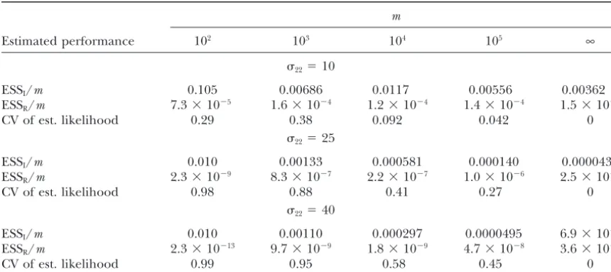
TABLE 1
The dependence of various performance statistics on the sample size when performing importance sampling
m
Estimated performance 102 103 104 105 ∞
22⫽10
ESSI/m 0.105 0.00686 0.0117 0.00556 0.00362
ESSR/m 7.3⫻10⫺5 1.6⫻10⫺4 1.2⫻10⫺4 1.4⫻10⫺4 1.5⫻10⫺4
CV of est. likelihood 0.29 0.38 0.092 0.042 0
22⫽25
ESSI/m 0.010 0.00133 0.000581 0.000140 0.0000434
ESSR/m 2.3⫻10⫺9 8.3⫻10⫺7 2.2⫻10⫺7 1.0⫻10⫺6 2.5⫻10⫺6
CV of est. likelihood 0.98 0.88 0.41 0.27 0
22⫽40
ESSI/m 0.010 0.00110 0.000297 0.0000495 6.9⫻10⫺6
ESSR/m 2.3⫻10⫺13 9.7⫻10⫺9 1.8⫻10⫺9 4.7⫻10⫺8 3.6⫻10⫺7
CV of est. likelihood 0.99 0.95 0.58 0.45 0
The parameters are as in Figure 3.
depend on the number of samples used. We show in putational effort is needed to implement these methods.
Finally, considering the values for finitemshows that if theappendixthat the importance sampling method is
more efficient than the rejection method. On the other ESSIis estimated from the simulation output (which is
usually the only option), then it can be very seriously hand, it is much harder to assess the precision of the
resulting estimates. overestimated for smallm, leading to inappropriate
con-fidence in the amount of information in the resulting
In the appendix we define formally the concept of
effective sample size, ESSI and ESSR, as a measure of simulations. The reasons for this are described in the
appendix, but it is crucial to be aware of these potential the information content of samples generated by the
importance and rejection algorithms, respectively. In- pitfalls when implementing the method (for a fuller
discussion, seeStephensandDonnelly2000). On the
formally, ifmneutral samples are simulated for use in
Algorithm 3, the effective sample size ESSIcorresponds other hand, the rejection probability, and hence ESSR,
is much more reliably estimated for smallm.In practice, to the number of independent samples under selection,
which would have the same information content as the while one should use the importance sampling
algo-rithm, it would be prudent, and conservative, to estimate
msamples used in the importance sampling algorithm.
ESSR is the expected number of independent samples ESSR from the simulation output and then to use this
as a lower bound on ESSI.
generated by the rejection method.
Care is needed, on several fronts, in the implementa- In view of the substantial computational burden in
applying our approach, it is natural to ask whether there tion of the methods in this article. Table 1 gives
esti-mates of the ratio of ESSI and ESSR to the number of are easier alternatives.
Consider first the problem of simulating samples, or simulated neutral samples for various levels of selection
in the deleterious alleles model. Several points are note- summary statistics, from the selected model. An
alterna-tive would be to simulate the evolution of the whole worthy. Considering the final column, we note that the
importance sampling method is more efficient (as population forward in time for a sufficiently long period
and then simply to take a sample from it. One difficulty
proved in theappendix) and in general requires about
an order of magnitude fewer samples than the rejection with this approach is that it is difficult to be sure how
long the simulation should be run to ensure that the method to gain the same information. Second,
espe-cially for more intense selection, the effective sample population allele frequencies are at stationarity under
mutation-selection-drift equilibrium. In practice it is sizes are small. To estimate the distribution of sample
statistics, one might want the equivalent of 103 or per- also not clear how to choose the size of the population
to be simulated. Clearly the computational burden
in-haps 104 independent samples under selection. Using
Algorithm 3, importance sampling would require the sim- creases substantially with the population size: more work
is required in simulating each generation, and more ulation of order 106, 108, and 109 neutral samples, for
22 ⫽ 10, 25, and 40, respectively, to have as much generations will be required to approximate stationarity
in a larger population. Implementation of the forward
information as of order 103independent samples from
sta-tionarity been achieved, and is the population size large hood surfaces can be a valuable tool in understanding the pitfalls of different approaches.
enough?), which cannot be verified without more
simu-Comparisons of likelihoods based on the full data with lation (for more generations and/or for larger
popula-those for simpler methods based on summary statistics tion sizes). In contrast, the formula (4) on which our
gives a useful sense of the amount of information lost method is based is exact for stationarity. Unless selection
by the simpler methods. coefficients are large and interest focuses on a small
population, our algorithms for simulation seem
prefera-From the perspective of classical statistics, the availability ble to forward simulation of the population.
of the likelihood surface immediately allows the use of A second alternative would be to use the ancestral
maximum-likelihood estimators for parameters. These
selection graph developed for genic selection by
Neu-would be expected to have good properties, at least
hauserandKrone(1997) or its generalization to
arbi-for large data sets, but the usual large-sample statistical
trary diploid selection inDonnellyandKurtz(1999).
theory, which, for example, allows the construction of One consequence of these methods is to extend
coales-confidence intervals for parameters from likelihood sur-cent approaches to simulation to nonneutral models.
faces or the testing via generalized-likelihood-ratio
statis-Informally, one first simulates the so-called ancestral tics of nested models, does not obviously apply for
popu-selection graph back to the “ultimate ancestor,” then lation genetics data. An alternative approach to interval
chooses the type of the ultimate ancestor appropriately, estimation would be through the use of a parameteric
and then simulates forward through the graph, with bootstrap (DavisonandHinkley1997). This study of
additional randomization, to obtain the sample. A seri- second-order properties of likelihoods for genetics
ous impediment to its use for general models is that models, while growing, is in its infancy. (Simulation
the distribution of the type of the ultimate ancestor is approaches are, for example, almost prohibitively
com-not known. For the models we are considering, however, putationally intensive.) In the case of models with
selec-it is known. Simply put n ⫽ 1 in (4). Our Algorithm 1 tion, it does not yet seem clear how best to construct
could then be used to choose the type of the ultimate confidence intervals.
ancestor. We noted earlier that very similar amounts of We applied our method to two data sets, in which
computation are needed for a sample of size 1 as for a purifying, respectively balancing, selection might
plausi-sample of arbitrary size. Use of the ancestral selection bly be thought to be operating. In practice, at least in
graph for simulation in these models is thus inefficient: a classical statistical framework, it would be appropriate
in simulating the type of the ultimate ancestor, one may to settle on a selective model before rather than after
as well simulate the entire sample of n; the effort of seeing the data. Our principal aim here was illustrative.
simulating the ancestral selection graph (which can be For a formal analysis one could use part or all of the
substantial, unless selective intensities are small) and data to suggest a particular model and then fit the model
going forward superimposing mutations is wasted. Simi- on additional data. There may also be some value
infor-lar comments apply to the methods of Slade (2000), mally in asking about what levels of particular sorts of
which use the ancestral selection graph to approximate selection might be consistent with observed data. For
likelihoods for two-locus models with selection. purifying selection there is also the question of which
Traditional approaches to inference in genetics mod- allele is the wild type. This could be regarded as part
els, based on one-dimensional summary statistics, often of the model choice and, for example, be based on
ignore much of the information in data. For single-locus data that are not subsequently used to fit the model.
Alternatively, if primary interest is in whether purifying data, where information is limited anyway by
evolution-selection is acting at all, rather than on which alleles it ary variability, this can be unhelpful. Within the context
is acting, it would be appropriate to evaluate the likeli-of a particular genetics model, efficient inference
(ei-hood by summing over all possible choices of the wild-ther estimation of parameters, hypothesis testing, or
type allele. This could be done at substantial computa-model comparison) requires evaluation of the
likeli-tional cost directly, but it would be easier to apply the hood function, and there has been considerable recent
results ofJoyce(1994).
interest in computationally intensive methods for
approx-While our approach to approximating likelihoods is imating likelihoods under various evolutionary models
computationally intensive, it seems the only one cur-(Stephens2001). In these problems, the ability to
ap-rently practicable. Except for very small sample sizes, proximate the likelihood had several important
conse-the naive approach of simulating samples for a grid of quences:
parameter values and for each set of parameter values
It immediately allows for Bayesian analyses, which have approximating the likelihood by counting the
propor-proved helpful in several contexts within population tion of times the data arise is unworkable. (For example,
genetics. for the Gundlach-Bundschu data, likelihood values are
For differing computational methods for approximat- of order 10⫺17, so thatⵑ1019simulated samples would be
likeli-value, with each such simulated sample itself requiring crosatellite mutation processes. There are some types
major computational effort, as discussed above.) of data (including those analyzed above) for which they
All of the methods described here apply to panmictic are applicable or at least are reasonable approximations.
populations of constant size. No theoretical results anal- It would be nice to extend our approach to more
realis-ogous to (4) are available for other demographic mod- tic models for mutation. At present, however, the
re-els. It is well known that certain forms of population quired theoretical results are not available (Donnelly
demography can produce patterns in data that are simi- andKurtz1999).
lar to those produced by particular forms of selection We thank A. Kong and M. Stephens for valuable discussions. P.D. was (Hudson1996). When analyzing only a single locus, it supported in part by UK Engineering and Physical Science Research Council Advanced Fellowship B/AF/1299 and grant GR/M14197, UK is thus difficult or impossible to separate demographic
Biotechnology and Biological Sciences Research Council grant 43/ effects from natural selection. This is a general problem,
MMI09788, and National Science Foundation grant DMS 9505129. common to all methods for analyzing single-locus data
M.N. was supported in part by Naturvetenskapliga forskningsra˚det sets. In particular, interpretation of parameter estimates
grant B-AA/BU 12026 and by the Erik-Philip So¨rensen Foundation. from our methods is only sensible for populations that P.J. was supported in part by NSF grants DMS-96-26764 and
DMS-00-have been at least approximately panmictic and of con- 72198.
stant size. As genome-wide data sets documenting intra-species variation become more common, it should be possible to separate demographic effects (which will
LITERATURE CITED
influence all loci) from selection at particular loci. For
Bernardo, J. M.,andA. F. M. Smith,1994 Bayesian Theory.Oxford the two data sets that we considered, we note thatKeith
University Press, Oxford.
et al.(1985) found almost identical frequency distribu- Davison, A. C.,andD. V. Hinkley,1997 Bootstrap Methods and Their
tions in several different locations in California, and Application.Cambridge University Press, Cambridge, UK.
Donnelly, P.,1986 Partition structures, Polya urns, and the Ewens
Qiuet al.(1997) tested their subpopulations for
inho-sampling formula, and the ages of alleles. Theor. Popul. Biol.
mogeneity before pooling. 30:271–288.
The methods discussed in this article are computa- Donnelly, P.,andT. G. Kurtz,1999 Genealogical processes for
Fleming-Viot models with selection and recombination. Ann. tionally intensive. Our general view is that
computa-Appl. Prob.9:1091–1148.
tional power is increasing and that given the cost and Donnelly, P.,andS. Tavare´,1987 The population genealogy of the effort required to collect data, there should not be con- infinitely-many neutral alleles model. J. Math. Biol.25:381–391.
Ethier, S. N.,andT. G. Kurtz,1994 Convergence to Fleming-Viot cern over analyses that take, say, hours or days, on
mod-processes in the weak atomic topology. Stoch. Proc. Appl. 54:
ern workstations. One positive feature of the methods
1–27.
developed here for likelihood surfaces is that the com- Ewens, W. J.,1972 The sampling theory of selectively neutral alleles. Theor. Popul. Biol.3:87–112.
putational burden does not depend much on the
sam-Ewens, W. J.,1990 Population genetics theory—the past and the ple size. (In fact, it decreases slightly as the sample size
future, pp. 177–227 in Mathematical and Statistical Development
increases.) of Evolutionary Theory, edited byS. Lessard.Kluwer Academic,
Dordrecht, The Netherlands. Both the rejection and importance sampling
algo-Grote, M. N.,andT. P. Speed,2001 Approximate Ewens formulae rithms for simulation avoid the need to evaluate the
for symmetric overdominance selection. Ann. Appl. Prob. (in
constantCdefined at (3). (It conveniently cancels from press).
Haldane, J. B. S.,1927 A mathematical theory of natural and artifi-numerator and denominator of both the rejection
prob-cial selection. V. Selection and mutation. Proc. Camb. Philos. ability and the importance weights.) In contrast, use of
Soc. Biol. Sci.23:838–844.
(4) to derive likelihoods for parameters such as the Hartl, D. L.,andS. A. Sawyer,1991 Inference of selection and
mutation rate and the strength of selection requires recombination from nucleotide sequence data. J. Evol. Biol.4:
519–532.
explicit evaluation ofC. As we noted, the obvious
ap-Hoppe, F. M.,1984 Polya-like urns and the Ewens sampling formula.
proach of simulating neutral populations and averaging J. Math. Biol.20:91–99.
the values of exp((X)) requires care because the distri- Hudson, R. R.,1996 Molecular population genetics of adaptation, pp. 291–309 inAdaptation, edited byM. R. RoseandG. V. Lauder.
bution of exp((X)) is extremely skewed to the right.
Academic Press, San Diego.
As a consequence, very large numbers of simulations Joyce, P.,1994 Likelihood ratios for the infinite alleles model. J.
from the neutral model are needed to gain any precision Appl. Prob.31:595–605.
Joyce, P.,1995 Robustness of the Ewens sampling formula. J. Appl. in evaluation ofC.In some settings, it can be evaluated
Prob.32:609-622.
by other means. We used population genetics theory Joyce, P.,1998 Partition structures and sufficient statistics. J. Appl.
and numerical integration for one of our examples and Prob.35:622–632.
Joyce, P.,andS. Tavare´,1995 The distribution of rare alleles. J. note a vast improvement (Figure 9).
Math. Biol.33:602–618.
A major weakness of the approach developed here is Keith, T. P., L. D. Brooks, R. C. Lewontin, J. C. Martı´nez-Cruzado
the restriction imposed on the mutation mechanism, andD. L. Rigby,1985 Nearly identical distributions of xanthine
dehydrogenase in two populations of Drosophila pseudoobscura.
namely that the type of a mutant does not depend on
Mol. Biol. Evol.2:206–216. the type of its parent. Our methods do not apply, for
Kong, A., J. LiuandW. H. Wong,1994 Sequential imputations and example, to effectively all models for mutation at the Bayesian missing data problems. J. Am. Stat. Assoc.89:278–288.
mi-Department of Mathematics, University of Southern California, m, of samples taken. (This is analogous to the fact that Los Angeles.
the rejection method will typically require many
rejec-Neuhauser, C.,andS. M. Krone,1997 The genealogy of samples
in models with selection. Genetics145:519–534. tions for each accepted sample.)
Qiu, W. G., E. Bosler, J. Campbell, G. Ugine, I. Wanget al., 1997 A serious danger with the importance sampling A population genetic study ofBorrelia burgdorferisensu stricto from
scheme occurs in settings when the distribution of the eastern Long Island, New York, suggested frequency-dependent
selection, gene flow and host adaptation. Hereditas127:203–216. weightsihas a heavy right tail: loosely, when most of
Ripley, B. D.,1987 Stochastic Simulation.John Wiley & Sons, New the importance weights are relatively small and only York.
very occasional weights are substantial. In this case, the
Slade, P. F.,2000 Simulation of selected genealogies. Theor. Popul.
Biol.57:35–49. sample mean and variance of the sampled weights may
Stephens, M.,2001 Inference under the coalescent, pp. 213–238 seriously underestimate the true mean and variance, inHandbook of Statistical Genetics, edited byD. J. Balding, M. J.
with the effect being greater for the variance. Should
BishopandC. Cannings.John Wiley & Sons, Chichester, UK.
Stephens, M.,andP. Donnelly,2000 Inference in molecular popu- this occur, the estimated effective sample size could be lation genetics. J. R. Stat. Soc. B62:605–655. substantially larger than the true effective sample size,
Watterson, G. A.,1978 The homozygosity test of neutrality.
Genet-with the misleading effect of seriously overstating the ics88:405–417.
Watterson, G. A.,1987 Estimating the proportion of neutral mu- precision of the estimation method. Assessing whether
tants. Genet. Res.501:155–163. this might be the case is difficult. One needs to know
Wright, S.,1931 Evolution in Mendelian populations. Genetics16:
whether substantially longer simulation runs would 97–159.
Wright, S.,1949 Adaptation and selection, pp. 365–389 inGenetics, throw up some importance weights that were
apprecia-Palaeontology, and Evolution, edited byG. L. Jepson, G. G. Simpson bly larger than those already seen.
andE. Mayr.Princeton University Press, Princeton, NJ.
Writemax⬅exp(max) for the largest possible impor-Communicating editor:S. Tavare´ tance weight. The acceptance probability in the
rejec-tion method is E(i)/max. (Observe, incidentally, that
E(i)⫽ C.) Ifmneutral samples are generated for the
rejection method, the expected number of accepted
APPENDIX
samples is
Rejectionvs.importance sampling for estimating the
distribution of sample statistics:The rejection scheme ESS
R⫽
m
max/E(i). (A2) has the advantage that it generates an independent
sam-ple, of known size m, of values of the sample statistic
The effective sample size ESSR has the interpretation
under the nonneutral model. Just as in standard
simula-that if the rejection method is used, and m neutral
tion problems, the accuracy of the estimated
distribu-samples are generated, then the precision of estimation
tion can be assessed in terms of the sample sizem.On
will be roughly that based on ESSRindependent samples.
the other hand, as our examples later illustrate, each
Of course, in an application of the rejection method
of the m nonneutral samples may actually involve the
one actually knows how many independent samples are simulation, and rejection, of a large number (of order
available. Nonetheless, we can compare the expected
104in our examples) of neutral samples.
performance of the two methods on the basis of the In using all the simulated neutral samples, the
impor-same number of initial neutral samples. Writing φ()
tance sampling scheme is in some sense more efficient
for the density ofi, than the rejection method. On the other hand, its
accu-racy is much more difficult to assess.Konget al.(1994) E(i)2⫽
冮
∞
0
2φ()d ⱕ
冮
∞
0
maxφ()d ⫽ maxE(i).
note that the importance sample of sizemis comparable
to an independent sample of size (A3)
It follows that ESSI⬅
m
1⫹CV2, (A1)
Var(i)ⱕ maxE(i)⫺(E(i))2,
where CV2⫽Var(i)/(E(i))2is the squared coefficient
which in turn implies of variation of the importance weights. The sample
mean and sample variance of the importance weights ESS
1ⱕ ESSR. (A4)
i,i⫽ 1, 2, . . . , m, can be used to estimateE(i) and
Var(i), respectively, and hence to estimate CV2. An Further, in the settings (as here) in which Var(i) is
substantial, there is likely to be considerable slack in
estimate of the effective sample size EESI can then be
calculated from (10), with the interpretation that the the inequality (A3) and hence in (A4). The inequality
(A4) confirms that the importance sampling method is accuracy of the estimated distribution will be roughly
the same as that obtained from ESSIindependent sam- more efficient, possibly substantially so.
Finally we note that in the importance scheme, an ples from the nonneutral model. In settings such as
those considered later in the article, the effective sample alternative would be that for each simulated neutral
sample X(i)
n , one could generate independent
tions of the population composition given this particular than the one described above. (While the weights will have lower variance, which is helpful, this does not offset sample and assign as a weight toX(i)
n the average of the
weights calculated for each of these simulated popula- the lower number ofX(i)
n that can be simulated for the
![Remifentanil versus fentanyl for analgesia based sedation to provide patient comfort in the intensive care unit: a randomized, double blind controlled trial [ISRCTN43755713]](data:image/gif;base64,R0lGODlhAQABAIAAAP///wAAACH5BAEAAAAALAAAAAABAAEAAAICRAEAOw==)