Modeling and analysis of software aging and rejuvenation

Modeling and Analysis of Software Aging and Rejuvenation

Kishor S. Trivedi, Kalyanaraman Vaidyanathan and Katerina Goˇseva-Popstojanova

Center for Advanced Computing & Communication

Dept. of Electrical & Computer Engineering

Duke University

Durham, NC 27708, USA

f

kst,kv,katerina

g

@ee.duke.edu

Abstract

Software systems are known to suffer from outages due to transient errors. Recently, the phenomenon of “software aging”, one in which the state of the software system de-grades with time, has been reported. To counteract this phe-nomenon,a proactive approach of fault management, called “software rejuvenation”, has been proposed. This essen-tially involves gracefully terminating an application or a system and restarting it in a clean internal state. In this paper, we discuss stochastic models to evaluate the effec-tiveness of proactive fault management in operational soft-ware systems and determine optimal times to perform re-juvenation, for different scenarios. The latter part of the paper deals with measurement-based methodologies to de-tect software aging and estimate its effect on various system resources. Models are constructed using workload and re-source usage data collected from the UNIX operating sys-tem over a period of time. The measurement-based models are intended to help development of strategies for software rejuvenation triggered by actual measurements.

1. Introduction

Demands on software reliability and availability have in-creased tremendously due to the nature of present day ap-plications. They impose stringent requirements in terms of cumulative down time and failure free operation of soft-ware, since in many cases, the consequences of software failure can lead to huge economic losses or risk to human life. However, it is almost impossible to fully test and verify if a piece of software is bug-free. Testing software becomes harder if it is complex, and further if testing and debugging

This work was supported in part by the NSF, Telcordia, Alcatel and the DoD as a core project of the CACC, Duke University and by Cabletron Systems under an NCNI Fellowship.

cycle times are reduced due to smaller release time require-ments. Therefore, the residual faults have to be tolerated in the operational phase.

Traditional design diversity techniques for fault toler-ance in software systems, such as N-version programming and Recovery block, are inherently expensive to implement due to the multiple functionally equivalent variants of the software needed. Furthermore, recent studies have reported the transient nature of software failures [13, 18] for which design diversity is not very helpful. Transient failures typi-cally occur because of design faults in software which result in unacceptable erroneous states in the OS environment of the process. Hence, environment diversity, a generalization of system restart [13], has been proposed as a cheap yet effective technique for software fault-tolerance [16]. The basic idea here is to modify the operating environment of the running process.

Traditional fault tolerance techniques are reactive in na-ture and typically, environment diversity has been done so far on a corrective basis. On the other hand, proactive fault management, as the name implies, takes suitable corrective action to prevent a failure before the system experiences a fault. Although, this technique has been used ad hoc for long in physical systems, it has only recently gained recog-nition and importance.

Recently, the phenomenon of software aging [17], one in which error conditions actually accrue with time and/or load, has been observed. In systems with high reliabil-ity/availability requirements, software aging can cause out-ages resulting in high costs. Huang et. al.report this phe-nomenon in telecommunications billing applications where over time the application experiences a crash or a hang fail-ure [17]. Avritzer and Weyuker discuss aging in telecom-munication switching software where the effect manifests as gradual performance degradation [1]. Software aging has also been observed in widely-used software like Netscape and xrn.

called software rejuvenation has been proposed [17]. It in-volves stopping the running software occasionally, “clean-ing” its internal state and restarting it. Garbage collection, flushing operating system kernel tables, reinitializing inter-nal data structures are some examples of what cleaning the internal state of a software might involve. An extreme, but well known example of rejuvenation is a hardware reboot. It has been implemented in the real-time system collect-ing billcollect-ing data for most telephone exchanges in the United States [2]. A very similar technique called software capac-ity restoration, has been used by Avritzer and Weyuker in a large telecommunications switching software [1], where the switching computer is rebooted occasionally upon which its service rate is restored to the peak value. Grey [14] pro-posed performing operations solely for fault management in SDI (Strategic Defense Initiative) software which are in-voked whether or not the fault exists and called it opera-tional redundancy. Tai et. al. [23] have proposed and ana-lyzed the use of on-board preventive maintenance for max-imizing the probability of successful mission completion of spacecrafts with very long mission times. The necessity of performing preventive maintenance in a safety critical envi-ronment is evident from the example of aging in Patriot’s software [19]. The failure which resulted in loss of hu-man lives could have been prevented if the computer was restarted after each 8 hours of running time.

In this paper, we present the two approaches for ana-lyzing software aging and studying aging-related failures. Section 2 discusses the analytical modeling approach aimed at determining optimal times to perform software rejuve-nation, while Section 3 deals with the measurement based approach for detection and validation of the existence of software aging and also estimating its effect on system re-sources. Section 4 concludes the paper.

2. Analytical models

Preventive maintenance (PM) can be performed at suit-able times, such as when there is no load on the system, and thus typically results in lesser downtime and cost than the corrective approach. Even so, it incurs some overhead and if done more often than necessary will result in higher downtime/cost. Therefore, an important research issue is to determine the optimal times to perform preventive main-tenance of operational software systems. This section dis-cuses analytical models for quantitative analysis of software rejuvenation.

The accuracy of a modeling based approach is deter-mined by the assumptions made in capturing aging. In [17, 6, 7, 8, 23] only the failures causing unavailability of the software are considered, while in [20] only a gradually decreasing service rate of a software which serves transac-tions is assumed. In [9], however, both these effects of aging

are considered together in a single model. Models proposed in [17, 6, 7] are restricted to hypo-exponentially distributed time to failure. Those proposed in [8, 20, 23] can accom-modate general distributions but only for the specific aging effect they capture. Generally distributed time to failure, as well as the service rate being an arbitrary function of time are allowed in [9]. It has been noted [22] that transient failures are partly caused by overload conditions. Only the model presented in [9] captures the effect of load on aging. Existing models also differ in the measures being evalu-ated. In [8, 23] software with a finite mission time is consid-ered. In the [17, 6, 7, 9] measures of interest in a transaction based software intended to run forever are evaluated. Since all previous models except [8] and [23] are just special cases of the model presented in [9], in the rest of this section we deal with this model in more detail.

2.1 Preventive maintenance in transactions based software systems

The macro-states representation of the software behav-ior considered in [9] is presented in Figure 1. The state in which the software is available for service (albeit with de-creasing service rate) is denoted as state

A

. After failure a recovery procedure is started. In state

B

the software is re-covering from failure and is unavailable for service. Lastly, the software occasionally undergoes PM, denoted by state

C

. PM is allowed only from state

A

. Once recovery from failure or PM is complete, the software is reset to state

A

and is as good as new. From this moment, which constitutes a renewal, the whole process stochastically repeats itself.

B A C

Undergoing PM Recovering

Available

Figure 1. Macro-states representation of the software behavior

The model is based on the following assumptions. The system consists of a server type software to which trans-actions arrive at a constant rate . Each transaction re-ceives service for a random period. The service rate of the software is an arbitrary function measured from the last re-newal of the software (because of aging) denoted by

(). Therefore, a transaction which starts service at time

t

1, oc-cupies the server for a time whose distribution is given by

1;

e

;

R t t

1 ()dt

the one being processed) and any more arriving when the queue is full are lost. The service discipline is FCFS. The software fails with a rate

(), that is, the CDF of the time

to failure

X

is given by

F

X

(

t

)=1;

e

;

R t 0

()dt

. Times to recover from failure

Y

f and to perform PM

Y

rare random variables with associated general CDFs

F

Yf and

F

Yr re-spectively. The model does not require any assumptions on the nature of

F

Yf and

F

Yr. Only the respective expectations

f =

E

Y

f ]and

r =

E

Y

r

]are assumed to be finite. The service degradation and hang/crash failures are assumed to be stochastically independent processes. Their interdepen-dence, if it exists in the real system, can be approximated by using parametric dependence in the definitions of

()and

(). Further, the failure process is stochastically indepen-dent of the arrival process and any transactions in the queue at the time of failure or at the time of initiation of PM are assumed to be lost. Moreover, any transactions which arrive while the software is recovering or undergoing PM are also lost.

The effect of aging in the model may be captured by using decreasing service rate and increasing failure rate, where the decrease or the increase respectively can be a function of time, instantaneous load, mean accumulated load or a combination of the above.

()=

(

t

)and

()=

(

t

)

In this case, the service rate and the failure rate are simply functions of time. To model software sys-tems with no performance degradation, the combina-tion

()=

and

()=

(

t

)may be used. Further, to model software systems which undergo performance degradation but are always available, the special case of

()=

=0and

()=

(

t

)can be used.

()=

(

N

(

t

))and

()=

(

N

(

t

))

The service rate and the failure rate are functions of in-stantaneous load on the system, i.e., their value at time

t

depend on the number of transactions in the queue at that time

N

(

t

). This dependence is useful in capturing overload effects which especially influence the failure behavior.

()=

(

L

(

t

))and

()=

(

L

(

t

))

Since an idle software is not likely to age, service and failure rates are more realistically modeled as func-tions of the actual processing time rather than the total available time. Denote with

p

i

(

t

)

0

i

K

the probability that there are

i

transactions in the queue at time

t

given that the software is in state

A

. Let

L

(

t

)be

defined as

L

(

t

) = Z

t

=0 X

i

c

i

p

i

(

)

d

, where

c

i is a coefficient which expresses how being in state

i

influ-ences the degradation of the overall system. If

c

0

=0 and

c

i

=1for

i >

0then

L

(

t

)represents the average

amount of time the software is busy processing trans-actions in the interval(0

t

]. If

c

i

=1for

i

0, then

L

(

t

)=

t

given that the software is available.

We consider two policies which can be used to deter-mine the time to perform PM. Under the Policy I which is purely time-based, PM is initiated after a constant time

has elapsed since it was started (or restarted). Under Policy II, which is based on instantaneous load and time, a constant waiting period

must elapse before PM is attempted. After this time PM is initiated if and only if there are no trans-actions in the system. Otherwise, the software waits until the queue is empty upon which PM is initiated. The actual PM interval under Policy II is determined by the sum of PM wait

and the time it takes for the queue to get empty from that point onwards

B

. Since the latter quantity is dependent on system parameters and can not be controlled, the actual PM interval has a range

1).

Given the above behavioral model the following mea-sures are derived for each policy: steady state availability of the software

A

SS, long run probability of loss of a trans-action

P

loss, and expected response time of a transaction given that it is successfully served

T

res. The goal is to de-termine optimal values of

(PM interval under policy I and PM wait under policy II) based on the constraints on one or more of these measures.

2.1.1 Evaluation of measures

According to the model described above at any time

t

the software can be in any one of three states: up and available for service (state

A

), recovering from a failure (state

B

) or undergoing PM (state

C

). Letf

Z

(

t

)

t

0gbe a stochastic process which represents the state of the software at time

t

. Further, let the sequence of random variables

S

i

i >

0 rep-resent the times at which transitions among different states take place. Since the entrance times

S

i constitute renewal pointsf

Z

(

S

i

)

i >

0gis an embedded discrete time Markov chain (DTMC) with a transition probability matrix

P

given by:

P

=

2

4

0

P

AB

P

AC

1 0 0

1 0 0

3

5

:

(1)

The steady state probability iof the DTMC being in state

ii

2f

ABC

gis:

=

A B C

]=

1 2

1 2

P

AB

1 2

P

AC

:

(2)

since by assumption all transactions arriving while the soft-ware is either recovering or undergoing PM are lost. Fur-ther, the transactions already in the queue at the transition instant are also discarded. It can be shown that the pro-cessf(

Z

(

t

)

N

(

t

))

t

0gis a Markov regenerative pro-cess (MRGP). Transition to state

A

from either

B

or

C

con-stitutes a regeneration instant.

Let

U

be a random variable denoting the sojourn time in state

A

, and denote its expectation by

E

U

]. Expected sojourn times of the MRGP in states

B

and

C

are already defined to be

fand

r.

The steady state availability is obtained using the standard formulae from MRGP theory:

A

SS

=

Pr

fsoftware is in state

A

g

=

A

E

U

] B

f

+ C

r

+ A

E

U

]

:

(3)

The probability that a transaction is lost is defined as the ratio of expected number of transactions which are lost in an interval to the expected total number of transactions which arrive during that interval. Since the evolution of

f

Z

(

t

)

N

(

t

))

t >

0g in the intervals comprising of suc-cessive visits to state

A

is stochastically identical it suffices to consider just one such interval. The number of transac-tions lost is given by the summation of three quantities: (1) transactions in the queue when the system is exiting state

A

because of the failure or initiation of PM (2) transactions that arrive while failure recovery or PM is in progress and (3) transactions that are disregarded due to the buffer being full. The last quantity is of special significance since the probability of buffer being full will increase due to the de-grading service rate. It follows that the probability of loss is given by,

P

loss

= A

E

N

l ]+

B

f +

C

r + A Z 1 0

p

K (

t

)

dt

( B

f

+ C

r

+ A

E

U

])

(4)

where

E

N

l

]is the expected number of transactions in the buffer when the system is exiting state

A

. Equation 4 is valid only for policy II. Under policy I sojourn time in state

A

is limited by

, so the upper limit in the integral R

1 0

p

K

(

t

)

dt

is

instead of1.

Next we derive an upper bound on the mean response time of a transaction given that it is successfully served, denoted by

T

res. The mean number of transactions, de-noted by

E

, which are accepted for service while the soft-ware is in state

A

is given by the mean number of trans-actions which are not accepted due to the buffer being full, subtracted from the mean total number of transac-tions which arrive while the software is in state

A

, that

is,

E

=

E

U

]; Z

1

t=0

p

K (

t

)

dt

. Out of these

transac-tions, on the average,

E

N

l

] are discarded later because

of failure or initiation of PM. Therefore, the mean num-ber of transactions which actually receive service given that they were accepted is given by

E

;

E

N

l

]. The mean total amount of time the transactions spent in the system while

the software is in state

A

is

W

= Z 1 t=0 X i

ip

i

(

t

)

dt

. This time is composed of the mean time spent by the transac-tions which were served as well as those which were dis-carded, denoted as

W

S and

W

D, respectively; Therefore,

W

=

W

S +

W

D. The response time we are interested in is given by

T

res

=

W

S

=

(

E

;

E

N

l

]), which is upper bounded by

T

res

<

W

E

;

E

N

l ]

:

(5)

Behavior of the system in state

A

under policy I

For

Z

(

t

)=

A

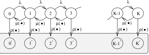
, the subordinated process, i.e., the process until a regeneration occurs, is determined by the queuing behavior of the software processing transactions. The pro-cess is terminated either by a failure (which can happen at any time) or by initiating PM which under policy I hap-pens at time

if the software has not failed by that time. Figure 2 shows the state diagram of the subordinated non-homogeneous process under policy I. Not included in the figure is the fact that at

t

=

, the subordinated process is terminated if it was not terminated before by a transition to an absorbing state (0

0

:::K

0 ). λ ρ( ) λ ρ( ) λ ρ( ) ρ( ) µ( ) ρ( ) λ ρ( ) µ( ) µ( ) µ( ) 3 3

’ 1’ ₂’ ’ _K-1’ _K’

0

0 1 2 K-1 K

Figure 2. Subordinated non-homogeneous CTMC for

t

By the above notation,

p

i

(

t

)is the probability that there are

i

transactions queued for service, which is also the probability of being in state

i

of the subordinated process at time

t

. Note that state

ii

= 0

1

:::K

is not to be confused with state

i

0

i

= 0

1

:::K

which was defined just to be able to evaluate the quantities of interest. As such, all the states under the shaded area of the process can be lumped into a single absorbing state.

Behavior of the system in state

A

under policy II

that PM will be initiated after time

has elapsed if and only if the buffer is empty. For

t

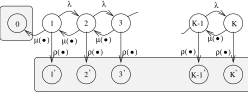
, exactly the same process of Figure 2 determines the behavior of the software. For

t >

, the process which models the behavior is shown in Figure 3. Observe that state 0now belongs to the set of absorbing states because PM will be initiated once the system becomes idle thus terminating the subordinated process.

λ

µ( ) λ

µ( ) µ( )

ρ( )

ρ( ) ρ( ) ρ( ) ρ( )

λ

µ( )

3

3

’ ₂’ ’ _K-1’ _K’

1

0 1 2 K-1 K

Figure 3. Subordinated non-homogeneous CTMC if

t >

Transient probabilities

p

i

(

t

)

i

= 0

1

:::K

and

p

i 0

(

t

)

i

0

=0 0

1

0

:::K

0

for both policies can be obtained by solving the systems of forward differential-difference equations given in [9]. In general they do not have a closed-form analytical solution and must be evaluated numerically. Once these probabilities are obtained, the rest of the quan-tities

P

AB,

P

AC,

E

U

]and

E

N

l

]can be easily computed [9] and then substituted into the equations (3), (4) and (5) to obtain the steady state availability

A

SS, the probability of transaction lost

P

lossand the upper bound on the response time of a transaction

T

resrespectively.

2.1.2 Numerical examples

We illustrate the usefulness of the presented model in deter-mining the optimum value of

(PM interval in the case of policy I and PM wait in the case of policy II) on the exam-ples adopted from [9].

First, service rate and failure rate are assumed to be func-tions of real time where

(

t

) is defined to be the hazard function of Weibull distribution, while

(

t

)is defined to be a monotone non-increasing function that approximates the service degradation. Figure 4 shows

A

ssand

P

lossfor both policies plotted against

for different values of the mean time to perform PM

r.

Under both policies, it can be seen that for any particular value of

, higher the value of

r, lower is the availability and higher is the corresponding loss probability. It can also be observed that the value of

which minimizes probability of loss is much lower than the one which maximizes avail-ability. In fact, the probability of loss becomes very high at values of

which maximize availability. For any specific value of

r, policy II results in a lower minima in loss

prob-ability than that achieved under policy I. Therefore, if the objective is to minimize long run probability of loss, such as in the case of telecommunication switching software, policy II always fares better than policy I.

Figure 5 shows

A

SS,

P

loss and upper bound on

T

res plotted against

under policy I.

Each of the figures contains three curves.

()and

() in the solid curve are functions of real time

(

t

)and

(

t

), whereas in the dotted curve they are functions (with the same parameters) of the mean total processing time

(

L

(

t

)) and

(

L

(

t

)). The dashed curve represents a third system in which no crash/hang failures occur

() = 0, but service degradation is present with

() =

(

t

). This experiment illustrates the importance of making the right assumptions in capturing aging because as seen from the figure, depend-ing on the forms chosen for

()and

(), the measures vary in a wide range.

3. Measurement-based estimation

In this Section we describe the measurement-based ap-proach for detection and validation of the existence of soft-ware aging. The basic idea is to periodically monitor and collect data on the attributes responsible for determining the health of the executing software, in this case the UNIX erating system. For quantifying the effect of aging in op-erating system resources, the metric Estimated time to ex-haustion is proposed. The earlier work [10] uses a purely time-based approach to estimate resource exhaustion times, whereas the the work recently presented in [25] takes into account the current system workload as well.

0.0 100.0 200.0 300.0 400.0

δ

0.990 0.991 0.992 0.993 0.994 0.995 0.996 0.997 0.998

Availability

I, 0.15 I, 0.35 I, 0.55 I, 0.85 II, 0.15 II, 0.35 II, 0.55 II, 0.85

0.0 50.0 100.0 150.0

δ

0.00 0.01 0.01 0.02 0.02 0.03 0.04

Loss Probability

I, 0.15 I, 0.35 I, 0.55 I, 0.85 II, 0.15 II, 0.35 II, 0.55 II, 0.85

Figure 4. Results for Experiment 1.

0 100 200 300 400 500

δ

0.990 0.992 0.995 0.997 1.000

Availability

real time Busy time no failure

0 100 200 300 400 500

δ

0.00 0.03 0.05 0.08 0.10

Loss Probability

real time busy time no failure

0 100 200 300 400 500

δ

0.0 1.0 2.0 3.0 4.0 5.0 6.0

Response Time

real time busy time no failure

Figure 5. Results of Experiment 2.

3.1. Time-based estimation

We thus obtain time-ordered values for each pfmMIB

object, constituting a time series for that object. Our objec-tive here is to detect aging or a long term trend (increasing or decreasing) in the values and also to study the nature of the variations in values. Furthermore, we attempt to relate failures during this period to the observed values and dis-cuss methods to quantify aging. Classical time series analy-sis techniques such as linear and periodic dependency anal-ysis, and trend detection and estimation [3] are used for our analysis.

3.1.1 Detection and validation of the existence of aging

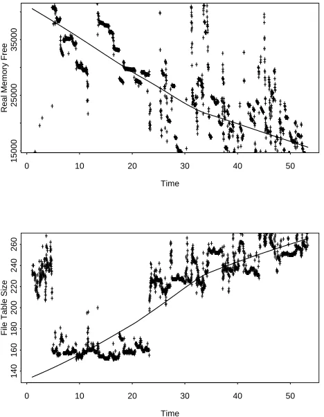
As mentioned previously, one of the primary objectives of the data analysis is to detect and validate the existence of aging. Detection of trends in operating system resource us-age and system activity is the approach followed. For the purposes of prediction, the slope of the trend is estimated. The primary trend detection technique used is smoothing of observed data by robust locally weighted regression, pro-posed by Cleveland [5]. Figure 6 shows the smoothed data superimposed on the original data points from the time se-ries of objects for Rossby. The smoothing technique is used only to get the global trend between outages and so the re-sulting smoothed data might not always follow the original data points. Amount of real memory free (plot 1) shows an overall decrease, whereas file table size (plot 2) shows

an increase. Plots of some other resources not discussed here also showed an increase or decrease. Once again, this corroborates the hypothesis of aging with respect to various objects.

The seasonal Kendall test [11] was applied to each of these time series to detect the presence of any global trends at a significance level,

, of 0.05. The associated statistic is listed in Table 1. With

Z

=1.96, all values in the table are such that the

H

0hypothesis that no trend exists is rejected.

Table 1. Seasonal Kendall test

Resource Name Rossby Jefferson Real Memory Free -13.668 -46.977

File Table Size 38.001 47.065 Process Table Size 40.540 38.537 Used Swap Space 15.280 31.660 No. of disk data blocks 48.840 13.673 No. of queues 39.645 13.476

3.1.2 Age quantification and estimation

Time

Real Memory Free

0 10 20 30 40 50

15000

25000

35000

Time

File Table Size

0 10 20 30 40 50

140

160

180

200

220

240

260

Figure 6. Non-parametric regression smooth-ing for Rossby objects

data with seasons [10]. A negative slope, as in the case of real memory, indicates a decreasing trend, whereas a posi-tive slope, as in the case of file table size, is indicaposi-tive of an increasing trend. Given the slope estimate, the table lists the estimated time to failure of the machine due to aging only with respect to this particular resource. The calculation of the time to exhaustion is done by using the initial intercept,

c

, the calculated slope,

m

, and a standard linear approxima-tion

y

=

mx

+

c

. The value of the intercept

c

is taken to be the mean of the initial 5 days. The minimum value for all the resources is zero.

A comparative effect of aging on different system re-sources can be obtained from the above estimates. For ex-ample, in machine Rossby, the resource used swap space has the highest slope and real memory free has the sec-ond highest slope. However, the estimated times to ex-haustion of both these resources is compared, real memory free has a lower time to exhaustion than used swap space. This is because of the difference in the initial and

maxi-mum/minimum values of these resources. Overall, it was found that the two resources file table size and process ta-ble size are not as important as used swap space and real memory free since they have a very small slope and high estimated times to failure due to exhaustion. Based on such comparisons, we can identify important resources to moni-tor and manage in order to deal with aging related software failures.

3.2. Time and workload-based estimation

The method discussed in the previous subsection as-sumes that accumulated use of a resource over a time period depends only on the elapsed time. However, it is intuitive that the rate at which a resource is consumed is dependent on the current workload. In this subsection, we discuss a measurement-based model to estimate the rate of exhaus-tion of operating system resources as a funcexhaus-tion of both time and the system workload recently presented in [25]. The SNMP-based distributed resource monitoring tool de-scribed previously was used for collecting operating system resource usage and system activity parameters (at 10 min intervals) for over 3 months. Only results for the data col-lected from the machine Rossby are discussed here. The longest stretch of sample points in which no reboots or fail-ures occurred were used for building the model. A semi-Markov reward model [24] is constructed using the data. First different workload states are identified using statisti-cal cluster analysis and a state-space model is constructed. Corresponding to each resource, a reward function based on the rate of resource exhaustion in the different states is then defined. Finally the model is solved to obtain trends and the estimated exhaustion rates and time to exhaustion for the resources.

3.2.1 Workload characterization and modeling

The following variables were chosen to characterize the sys-tem workload - cpuContextSwitch, sysCall, pageIn, and pa-geOut. Hartigan’s k-means clustering algorithm [15] was used for partitioning the data points into clusters based on workload. The statistics for the eleven workload clusters obtained are shown in Table 3. Clusters whose centroids were relatively close to each other and those with a small percentage of data points in them, were merged to simplify computations. This resulting clusters are

W

1

= f1

2

3g,

W

2

= f4

5g,

W

3

= f6g,

W

4

= f7g,

W

5

= f8g,

W

6

=f9g,

W

7

=f10gand

W

8

=f11g.

Table 2. Estimated slope and time to exhaustion for Rossby, Velum and Jefferson objects

Resource Initial Max Sen’s Slope 95% Confidence Estimated Time

Name Value Value Estimation Interval to Exhaustion (days)

Rossby

Real Memory Free 40814.17 84980 -252.00 -287.75 : -219.34 161.96 File Table Size 220 7110 1.33 1.30 : 1.39 5167.50 Process Table Size 57 2058 0.43 0.41 : 0.45 4602.30 Used Swap Space 39372 312724 267.08 220.09 : 295.50 1023.50

Jefferson

Real Memory Free 67638.54 114608 -972.00 -1006.81 : -939.08 69.59 File Table Size 268.83 7110 1.33 1.30 : 1.38 5144.36 Process Table Size 67.18 2058 0.30 0.29 : 0.31 6696.41 Used Swap Space 47148.02 524156 577.44 545.69 : 603.14 826.07

Table 3. Statistics for the workload clusters

Cluster Center % of

No. cpuConSw sysCall pgOut pgIn pts.

1 48405.16 94194.66 5.16 677.83 0.98

2 54184.56 122229.68 5.39 81.41 0.76

3 34059.61 193927.00 0.02 136.73 0.93

4 20479.21 45811.71 0.53 243.40 1.89

5 21361.38 37027.41 0.26 12.64 7.17

6 15734.65 54056.27 0.27 14.45 6.55

7 37825.76 40912.18 0.91 12.21 11.77

8 11013.22 38682.46 0.03 10.43 42.87

9 67290.83 37246.76 7.58 19.88 4.93

10 10003.94 32067.20 0.01 9.61 21.23

11 197934.42 67822.48 415.71 184.38 0.93

P = 2

6 6 6 6 6 6 6 6 4

0:00 0:16 0:22 0:13 0:26 0:03 0:17 0:03 0:07 0:00 0:14 0:14 0:32 0:03 0:31 0:00 0:12 0:26 0:00 0:10 0:43 0:00 0:11 0:02 0:15 0:36 0:06 0:00 0:10 0:22 0:09 0:03 0:03 0:07 0:04 0:01 0:00 0:00 0:85 0:00 0:07 0:16 0:02 0:54 0:12 0:00 0:02 0:07 0:02 0:05 0:00 0:00 0:92 0:00 0:00 0:00 0:31 0:08 0:15 0:23 0:08 0:15 0:00 0:00

3

7 7 7 7 7 7 7 7 5

The sojourn time distribution for each of the work-load states was fitted to either 2-stage hyper-exponential or 2-stage hypo-exponential distribution functions. The fit-ted distributions, shown in Table 4, were tesfit-ted using the Kolmogorov-Smirnov test at a significance level of 0.01.

3.2.2 Modeling resource usage

Two resources, usedSwapSpace and realMemoryFree, are considered for the analysis, since the previous time-based

Table 4. Sojourn time distributions

State Sojourn Time Distribution,F(t)

W1 1;1:602919e ;0:9t

+0:6029185e

;2:392739t W

2

1;0:9995e

;0:4459902t

;0:0005e

;0:007110071t W3 1;0:9952e

;0:3274977t

;0:0048e

;0:0175027t W

4

1;0:841362e

;0:3275372t

;0:158638e

;0:03825429t

W5 1;1:425856e ;0:56t

+0:4258555e ;1:875t W

6

1;0:80694e

;0:5509307t

;0:19306e

;0:03705756t

W7 1;2:86533e ;1:302t

+1:86533e ;2t W8 1;0:9883e

;0:2655196t

;0:0117e

;0:02710147t

analysis suggested that they are critical resources. For each resource, the reward function is defined as the rate of cor-responding resource exhaustion in different states. The true slope (rate of increase/decrease) of a resource at every workload state is estimated by using Sen’s non-parametric method [25]. Table 5 shows the slopes with 95% confi-dence intervals. It was observed that slopes in a given

work-Table 5. Slope estimates (in KB/10 min)

usedSwapSpace realMemoryFree

State Slope 95 % Conf. Slope 95 % Conf.

Est. Interval Est. Interval

W1 119.3 5.5 - 222.4 -133.7 -137.7 - -133.3 W

2 0.57 0.40 - 0.71 -1.47 -1.78 - -1.09 W3 0.76 0.73 - 0.80 -1.43 -2.50 - -0.62 W

4 0.57 0.00 - 0.69 -1.23 -1.67 - -0.80

W5 0.78 0.75 - 0.80 0.00 -5.65 - 6.00

W

6 0.81 0.64 - 1.00 -1.14 -1.40 - -0.88

W7 0.00 0.00 - 0.00 0.00 0.00 - 0.00

W8 91.8 72.4 - 111.0 91.7 -369.9 - 475.2

that state are almost the same. Further, the slopes across different workload states are different and generally higher the system activity, higher is the resource utilization. This validates the assumption that resource usage does depend on the system workload and the rates of exhaustion vary with workload changes. It can also be observed from Ta-ble 5 that the slopes for usedSwapSpace in all the workload states are non-negative, and the slopes for realMemoryFree are non-positive in all the workload states except in one. It follows that usedSwapSpace increases whereas realMem-oryFree decreases over time which validates the software aging phenomenon described earlier in the paper.

3.2.3 Results

The semi-Markov reward model was solved using the SHARPE [21] tool developed at Duke University. The slope for the workload-based estimation is computed as the expected cumulative reward rate at steady state from the model. As in the case of time based estimation, the times to resource exhaustion is computed using the linear formula

y

=

mx

+

c

, where

m

is the slope and

c

is the intercept or the initial values and

y

is the final (maximum or minimum) value.

Figures 7 shows the time plots of usedSwapSpace in ma-chine Rossby along with the workload and time based esti-mations, while Table 6 gives the estimates for the slope and

Estimations of usedSwapSpace

Time (in days)

usedSwapSpace in KB

0 10 20 30 40

10000

20000

30000

40000

50000

Actual usedSwapSpace Workload based estimation 95% upper confidence level 95% lower confidence level TIme based estimation

Figure 7. Time plot and trend estimations of resourceusedSwapSpacein machine Rossby

time to exhaustion for both usedSwapSpace and realMemo-ryFree. It can be seen that workload based estimations gave a lower time to resource exhaustion than those computed using time based estimations. Since the machines failures

due to resource exhaustion were observed much before the times to resource exhaustion estimated by the time based method, it follows that the workload based approach results in better estimations.

3.2.4 Extensions of the measurement based approach

A possible extension of this work could be to consider the system workload in a more fine-grained manner by deter-mining the effect of each individual process on particular resource consumption. Further, for a more general failure prediction, the combined effect of aging, periodic compo-nent and transient compocompo-nent of resource usage need to be modeled and understood. Additionally, the interaction and correlation between the usage of various resources and their impact on system availability remains to be explored. It is precisely for these reasons that the estimated times of fail-ures done this way do not fully explain the actual times of failure observed on various machines.

4. Conclusions

In this paper, we have motivated the need for pursuing preventive maintenance in operational software systems on scientific basis rather than on the current ad-hoc practice. Thus, an important research issue is to determine the opti-mal times to perform the preventive maintenance. In this regard, we discuss the two possible approaches, analytical modeling and measurement based approach.

In the first part of the paper, we discuss analytical models for evaluating the effectiveness of preventive maintenance in operational software systems which experience aging. The aim of the analytical modeling approach is determin-ing the optimal times to perform rejuvenation considerdetermin-ing the tradeoffs of maximizing availability and minimizing the probability of loss or the response time of a transaction.

Table 6. Estimates for slope (in KB/10 min) and time to exhaustion (in days) forusedSwapSpaceand

realMemoryFree

Method usedSwapSpace realMemoryFree

of Slope 95 % Conf. Est. Time to Slope 95 % Conf. Est. Time to

Estimation Estimate Interval Exhaustion Estimate Interval Exhaustion

Time based 0.787 0.786 - 0.788 2276.46 -2.806 -3.026 - -2.630 60.81

Workload based 4.647 1.191 - 7.746 453.62 -3.386 -9.968 - 2.592 50.39

References

[1] A. Avritzer and E. J. Weyuker. Monitoring Smoothly Degrad-ing Systems for Increased Dependability. Empirical Software

Eng. Journal, Vol.2, No.1, pages 59-77, 1997.

[2] L. Bernstein. Text of Seminar Delivered by Mr. Bernstein.

University Learning Center, George Mason University,

Jan-uary 29, 1996.

[3] G. E. P. Box, G. M. Jenkins and G. C. Reinsel. Time Series

Analysis: Forecasting and Control. Prentice Hall, Englewood

Cliffs, NJ, 1994.

[4] J.D. Case, M. Fedor, M. L. Schoffstall, C. Davin, M. T. Rose and K. McCloghrie. Simple Network Management Protocol. RFC 1157, May 1990.

[5] W. S. Cleveland. Robust Locally Weighted Regression and Smoothing Scatterplots. Journal of the American Statistical

Association, 74(368):829-836, December 1979.

[6] S. Garg, A. Puliafito and K. S. Trivedi. Analysis of Software Rejuvenation Using Markov Regenerative Stochastic Petri Net. In Proc. of the Sixth Intl. Symposium on Software

Relia-bility Engineering, pages 180-187, Toulouse, France, October

1995.

[7] S. Garg, Y. Huang, C. Kintala and K.S. Trivedi, Time and load based software rejuvenation: policy, evaluation and op-timality. Proc. First Fault-tolerant Symposium, Dec. 22-25, Madras, India, 1995.

[8] S. Garg, Y. Huang and C. Kintala, K.S. Trivedi, Minimiz-ing Completion Time of a Program by CheckpointMinimiz-ing and Rejuvenation. Proc. 1996 ACM SIGMETRICS Conference, Philadelphia, PA, pp. 252-261, May 1996.

[9] S. Garg, A. Puliafito, M. Telek and K. S. Trivedi. Analysis of Preventive Maintenance in Transactions Based Software Sys-tems. IEEE Trans. on Computers, pages 96-107, Vol. 47, No. 1, January 1998.

[10] S. Garg, A. van Moorsel, K. Vaidyanathan and K. S. Trivedi. A Methodology for Detection and Estimation of Software Ag-ing. In Proc. of the Ninth Intl. Symposium on Software

Re-liability Engineering, pages 282-292, Paderborn, Germany,

November 1998.

[11] R. O. Gilbert. Statistical Methods for Environmental

Pol-lution Monitoring. Van Nostrand Reinhold, New York, NY,

1987.

[12] J. Gray. Why do Computers Stop and What Can be Done About it? In Proc. of 5th Symposium on Reliability in

Dis-tributed Software and Database Systems, pages 3-12, January

1986.

[13] J. Gray and D. P. Siewiorek. High-Availability Computer Systems. IEEE Computer, pages 39-48, September 1991. [14] B. O. A. Grey. Making SDI Software Reliable Through

Fault-Tolerant Techniques. Defense Electronics, pages 77-80, 85-86, August 1987.

[15] J. A. Hartigan. Clustering Algorithms. New York:Wiley, 1975.

[16] Y. Huang, P. Jalote and C. Kintala. Two Techniques for Tran-sient Software Error Recovery. Lecture Notes in Computer

Science, Vol. 774, pages 159-170. Springer Verlag, Berlin,

1994.

[17] Y. Huang, C. Kintala, N. Kolettis and N. D. Fulton. Software Rejuvenation: Analysis, Module and Applications. In Proc. of

25th Symposium on Fault Tolerant Computer Systems, pages

381-390, Pasadena, California, June 1995.

[18] I. Lee. Software Dependability in the Operational Phase. PhD. thesis, Department of Electrical and Computer Engi-neering, University of Illinois, Urbana-Champaign, IL, 1995. [19] E. Marshall. Fatal Error: How Patriot Overlooked a Scud.

Science, page 1347, March 13, 1992.

[20] A. Pfening, S. Garg, A. Puliafito, M. Telek and K. S. Trivedi, Optimal rejuvenation for tolerating soft failures, Performance

Evaluation, Vol. 27 & 28, October 1996, North-Holland, pp.

491-506.

[21] R. A. Sahner, K. S. Trivedi and A. Puliafito. Perfor-mance and Reliability Analysis of Computer Systems - An Example-Based Approach Using the SHARPE Software Pack-age. Kluwer Academic Publishers, Norwell, MA, 1996.

[22] M. Sullivan and R. Chillarege. Software Defects and Their Impact on System Availability - A Study of Field Failures in Operating Systems. In Proc. 21st IEEE Intl. Symposium on

Fault-Tolerant Computing, pages 2-9, 1991.

[23] A. T. Tai, S. N. Chau, L. Alkalaj and H. Hecht. On-Board Preventive Maintenance: Analysis of Effectiveness and Opti-mal Duty Period. In 3rd Intl. Workshop on Object Oriented

Real-time Dependable Systems, Newport Beach, CA,

Febru-ary 1997.

[24] K. S. Trivedi, J. K. Muppala, S. P. Woolet and B. R. Haverkort. Composite Performance and Dependability Anal-ysis. In Performance Evaluation, 14, pages 197-215, 1992. [25] K. Vaidyanathan and K. S. Trivedi. A Measurement-Based

Model for Estimation of Resource Exhaustion in Operational Software Systems. In Proc. of the Tenth IEEE Intl.

Sympo-sium on Software Reliability Engineering, pages 84-93, Boca