Smart Water: Short-Term Forecasting Application in Water Utilities

(1)

University of Windsor University of Windsor

Scholarship at UWindsor

Electronic Theses and Dissertations Theses, Dissertations, and Major Papers

2019

Smart Water: Short-Term Forecasting Application in Water Utilities

Mo'tamad Bata University of Windsor

Follow this and additional works at: https://scholar.uwindsor.ca/etd

Recommended Citation Recommended Citation

Bata, Mo'tamad, "Smart Water: Short-Term Forecasting Application in Water Utilities" (2019). Electronic Theses and Dissertations. 7685.

https://scholar.uwindsor.ca/etd/7685

(2)

Smart Water: Short-Term Forecasting Application in Water Utilities

By

Mo’tamad H. Bata

A Thesis

Submitted to the Faculty of Graduate Studies

through the Department of Civil and Environmental Engineering

in Partial Fulfillment of the Requirements for

the Degree of Master of Applied Science

at the University of Windsor

Windsor, Ontario, Canada

2019

(3)

Smart Water: Short-Term Forecasting Application in Water Utilities

By

Mo’tamad H. Bata

APPROVED BY:

___________________________________________________

J. Johrendt

Department of Mechanical, Automotive & Materials Engineering

___________________________________________________

T. Bolisetti

Department of Civil and Environmental Engineering

___________________________________________________

D. Ting, Co-Advisor

Department of Mechanical, Automotive & Materials Engineering

___________________________________________________

R. Carriveau, Advisor

Department Civil and Environmental Engineering

(4)

DECLARATION OF CO-AUTORSHIP / PREVIOUS PUBLICATION

I. Co-Authorship

I hereby declare that this thesis incorporates material that is result of joint research.

Chapters 3 & 4 of this thesis were completed under the supervision of Dr. Rupp Carriveau

and Dr. David Ting. In all cases, the key ideas, primary contributions, experimental design,

data analysis, interpretation, and writing were performed by the author. The contribution

of co-authors was primarily through the provision of checking and comments on the

literature review, methodology and modeling, results interpretation, providing feedback on

refinement of ideas, editing of the manuscript, and advice on selecting peer reviewed

journals for publication.

I am aware of the University of Windsor Senate Policy on Authorship and I certify that I

have properly acknowledged the contribution of other researchers to my thesis, and have

obtained written permission from each of the co-authors to include the above materials in

my thesis.

I certify that, with the above qualification, this thesis, and the research to which it refers,

is the product of my own work.

II. Previous Publication

This Thesis consists of three original papers that have been published / submitted or to be

submitted for publication in peer-reviewed journals, as follows:

Thesis

Chapter

Publication

Status

Chapter 3 Bata, Mo’tamad; Carriveau, Rupp; Ting, David S.-K.

2018. “Short-term Water Demand Forecasting Using

Nonlinear Autoregressive Artificial Neural Networks

(ANN)”. Engineering Application of Artificial

Intelligence.

(5)

Chapter 4 Bata, Mo’tamad; Carriveau, Rupp; Ting, David S.-K.

2018. “Hybrid Self Organizing Map and Regression Tree

Short-term Water Demand Forecasting Model”.

To be

submitted

I certify that I have obtained written permission from the copyright owner(s) to

include the above published material(s) in my thesis. I certify that the above material

describes work completed during my registration as a graduate student at the University of

Windsor.

III. I certify that, to the best of my knowledge, my thesis does not infringe upon anyone’s

copyright nor violate any proprietary rights and that any ideas, techniques, quotations, or

any other material from the work of other people included in my thesis, published or

otherwise, are fully acknowledged in accordance with the standard referencing practices.

Furthermore, to the extent that I have included copyrighted material that surpasses the

bounds of fair dealing within the meaning of the Canada Copyright Act, I certify that I have

obtained a written permission from the copyright owner(s) to include such material(s) in

my thesis and have included copies of such copyright clearances to my appendix.

I declare that this is a true copy of my thesis, including any final revisions, as

approved by my thesis committee and the Graduate Studies office, and that this thesis has

not been submitted for a higher degree to any other University or Institution.

I hereby certify that the thesis I am submitting is entirely my own original work

except where otherwise indicated. I am aware of the University's regulations concerning

plagiarism, including those regulations concerning disciplinary actions that may result

from plagiarism. Any use of the works of any other author, in any form, is properly

(6)

ABSTRACT

The unyielding interconnection between water and energy has made demand forecasting a necessity

for water utilities. Electricity prices driven by the time of use has impelled water utilities towards

short-term water demand forecasting. The progressive new Smart Water Grid platform has helped

water utilities in utilizing their Water Distribution Networks. This two-way platform has provided

developers and decision makers with robust models that rely on consumer feedback. Among these

models is the water demand forecasting models. Multitudinous demand forecasting methods have

been developed but none have utilized model implementation practicality. Utilities differ in size,

capacity, and interest. While small size utilities focus on model simplicity, larger utilities prioritize

model accuracy. This work focuses on a water utility located in Essex County, Ontario, Canada.

This study presents three papers that focus on investigation and evaluation of short-term water

demand forecasting techniques. The first paper compares water usage between two crops (tomatoes

and bell peppers) in an effort to evaluate a crop to crop forecast technique that relies on one crops

watering data in order to produce forecasts for another crop, The second paper examines the effect

of model type, input type, and data size on model performance and computational load. The third

paper proposes a new methodology where model performance is not sacrificed for model

(7)

DEDICATION

To Majeda and Hussein (Mom and Dad) for their endless support and continuously encouraging

(8)

ACKNOWLEDGMENTS

I would like to thank my advisors Dr. Rupp Carriveau and Dr. David S.-K. Ting as well as the

entire Turbulence and Energy Laboratory for their support, guidance, and patience they have shown

throughout my studies. I would also like to acknowledge my committee members Dr. Jennifer

Johrendt and Dr. Tirupati Bolisetti for their input along with Mr. Rodney Bouchard for providing

(9)

DECLARATION OF CO-AUTHORSHIP / PREVIOUS PUBLICATIONS ... iii

ABSTRACT ...v

DEDICATION ... vi

ACKNOWLEDGEMENTS ... vii

LIST OF TABLES ... xii

LIST OF FIGURES ... xiii

CHAPTER 1: Introduction ...1

Background ...1

Problem statement ...2

References ...3

CHAPTER 2: Forecasting Methodology ...5

Introduction ...5

C2C Methodology ...5

ANN Theory and Models...5

Forecasting methodology ...6

Nonlinear Autoregressive Models ...7

Hybrid Model ...8

References ...10

(10)

Nomenclature ...11

Introduction ...12

Study Area and Data ...13

Data Pre-processing ...16

Methods and Model development ...17

SARIMA Model ...17

Nonlinear Autoregressive with Exogenous inputs (NARX) ...18

Nonlinear Autoregressive (NAR) ...20

Baseline comparison and model performance ...20

Results and Discussion ...21

Linear vs. Nonlinear ...21

Single Input vs. Exogenous inputs ...22

Data span ...22

Computational Load ...23

Model Error Histogram ...24

Models application ...25

Conclusion ...27

Data Availability ...28

Acknowledgments...28

Conflicts of Interests ...28

References ...28

CHAPTER 4: Hybrid Self Organizing Map and Regression Tree Short-term Water

Demand Forecasting Model ...32

(11)

Methodology ...35

Data and Models ...38

Raw Data ...38

SOM Clustering Model ...40

RT Forecasting Model ...41

Model Performance ...41

Results and Discussion ...42

Models Overall Performance ...42

Model Selection ...43

Models Application ...44

Concluding Remarks ...46

Acknowledgements ...47

Conflicts of Interests ...47

References ...47

CHAPTER 5: Conclusions and Recommendations ...50

Summary ...50

Conclusion ...52

Recommendations ...53

APPENDICES

………...

..55

Appendix A: Permissions for Previously Published Work ...55

(12)

LIST OF TABLES

CHAPTER 3: Short-term Water Demand Forecasting Using Nonlinear

Autoregressive Artificial Neural Networks (ANN)

Table 1.

PCC measured for the predictors ……….……..… 15

Table 2.

Models overall performance ……….. 21

Table 3.

Computation load of forecasting models on training data ……….……… 23

Table 4.

Deployed models performance ……….. 25

CHAPTER 4: Hybrid Self Organizing Map and Regression Tree Short-

term Water Demand Forecasting Model

Table 1.

Highlights of linear and nonlinear short-term forecasting models ………...… 34

Table 2.

Spearman Correlation Coefficient ρ between the utility water Outflow and the predictors used in forecasting ……….. 39

(13)

LIST OF FIGURES

CHAPTER 1: Introduction

Figure 1.

Studied area location………..………….……… 3

CHAPTER 2: Forecasting Methodology

Figure 1.

Typical Artificial Neural Network Structure …..……… 6

CHAPTER 3: Short-term Water Demand Forecasting Using Nonlinear

Autoregressive Artificial Neural Networks (ANN)

Figure 1

.Utility water outflow m3_{/hr ……… 14}

Figure 2

. Ambient temperature (0_{C) ………..…….…..………..………... 15}

Figure 3

. Nearest Neighbour Hot Deck Imputation ….……….……….. 17

Figure 4.a

. NARX network algorithm ……..………..………… 19

Figure 4.b

. NAR network algorithm ………..………... 19

Figure 5

. Datasets distribution and outliers ……….……….. 24

Figure 6

. NARX-4m model error histogram ………..……….………….………. 25

Figure 7

. Models forecasting water demand 24 hours ahead (12/02/2107 3:00pm – 12/03/2017 2:00pm) …..………..……….….………. 26

Figure 8

. Models forecasting water demand 1 week ahead (12/02/2107 3:00pm – 12/09/2017 2:00pm) ...………..……….………. 27

CHAPTER 4: Hybrid Self Organizing Map and Regression Tree Short-

term Water Demand Forecasting Model

Figure 1.

2-dimentional (2D) SOM structure with number of neurons equal 2 ……….……… 36

(14)

Figure 3.

The utility hourly water outflow in m3_{/hr ……….……….. 38}

Figure 4.

SOM Weight positions – Clusters positions ……….………. 40

Figure 5.

Self-Organizing Maps output where 2 neurons (N) are used ..……… 41

Figure 6.

Models overall performance measured in NRMSE ………... 43

Figure 7.

Actual vs. predicted outflow for HYB-1hr and HYB-8hr for N=2 ………….….….. 44

Figure 8.

Figure 9.

(15)

CHAPTER 1 INTRODUCTION

Background

Existing conventional water networks are aging. Conventional distribution systems operate in a

one-direction supply process. Minimal feedback is provided from the demand side, i.e. the

consumers. With their centralized one-directional flow characteristics (Newbold J., 2009), these

systems are more prone to undetected failures and leaks. This can cause network disruptions and

waste water, which is discouraging in solving the two major water issues, scarcity and

security. Therefore, conventional water networks are unpredictable, economically

infeasible, energy inefficient, and hard to maintain and manage.

Over the past decade, the water security and scarcity issues have propelled governments, water

supply systems, and researchers to upgrade current networks and develop preventive

measures. These measures aim to avert the global population increases and the escalating global

warming effects; including but not limited to, droughts, fires, floods, and climate change.

New water management infrastructures have been successfully established to tackle the

aforementioned challenges. The new platform of tools, technologies, and models is known as the

Smart Water Grid (SWG). SWG is a two-way real time network with sensors and devices that

continuously and remotely monitor the Water Distribution System (WDS). Smart water meters can

monitor many different parameters such as pressure, quality, flow rate, temperature and

others (Martyusheva O., 2014). The gathered data is then used in various tools, models, and

decision make systems. For instance, data collected through pressure monitoring sensors can

be utilized to detect and locate damaged pipelines or system leaks. Compared to the conventional

water grid, SWG is more resilient, reliable, sustainable, and energy efficient.

The SWG approach can help solve one of the most complicated challenges in the Water

Distribution System (WDS), the imbalance between water supply and demand. Water supply,

measured by system production capacity, is usually a constant rate. On the other hand, the water

demand represented by water consumption varies throughout the day and from day to another. For

example, water demand is higher during daylight business hours than during night-time (Leirens et

al. 2010). Factors other than time of the day affect water demand, such as: number of consumers,

type of consumer, consumption seasonality, new technologies, etc. With this

(16)

keep the network in balance. The development of water demand forecasting models is essential in

developing pumping schedules and operating the network in balance (Fodya & Harley, 2014).

Researchers have extensively studied and proposed water demand forecasting models. A

rich review of over 30 papers published between the years of 2000 and 2010 was presented

by (Donkor et al. 2014). Models seemed to perform well on the studied data. However, one

common issue was found for the vast majority of the models, model practicality. Models were

deemed impractical due to: difficulty in acquiring input data, complexity in models architectures,

and ineffective development cost. Most models have focused more on model accuracy without any

consideration on how practical it would be for a specific utility to adapt such model. Here,

practicality is defined as model suitability for a specific utility. Model suitability is governed by

utility size, capacity, and interest to deploy a model. Small size utilities, for instance, may assign

more weight to model simplicity over accuracy. While, bigger utilities prioritize model accuracy

over model simplicity.

Problem statement

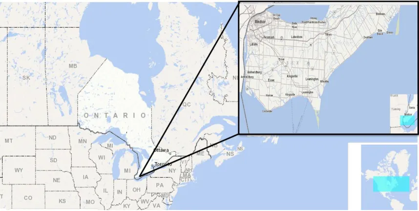
The Union Water Supply Systems (UWSS) located (see Figure 1) in Essex County, Ontario,

Canada, operates their network on reactive mode. When water levels in main reservoir drop,

operators turn pumps switches on. By doing that, operators respond to the demand in the past and

select pumps according to their knowledge and experience. UWSS faces new challenges where the

reactive mode is no longer efficient. UWSS receives continuous requests of additional water

demand by consumers. UWSS can supply the extra requested water demand, however, their

capability is constrained by the time of use. Moreover, UWSS is impacted by the energy time of

use prices fluctuation and the evolving renewable energy market penetration and its pressure on

big consumers.

UWSS can tackle the aforementioned challenges by switching into proactive mode. The anticipated

future demand is responded to within this mode instead of the past. Pumping schedules are prepared

ahead, pumps are selected accordingly, time of the use prices can be benefited from. Also, demand

peaks can be reduced which will result in less water and energy losses in the system. Proactive

mode is based on pre-knowledge of the demand patterns and can be achieved through short-term

water demand forecasting models.

The objective of this study was to propose and investigate short-term water demand forecasting

(17)

were adapted for this purpose. Once the models were developed, the next step was to evaluate their

performance and deployment practicality.

Figure 1. Studied area location

This study is made up of three research papers. The first paper (reviewed in chapter 2) has been

published in the Agriculture journal; Evaluation of Crop to Crop Water Demand Forecasting:

Tomatoes and Bell Peppers Grown in a Commercial Greenhouse (Rice et al. 2017) and proposed a

simple model where an end-user of only 80% of the utility consumers (i.e. commercial

greenhouses) are studied. This paper addresses the model complexity and practicality issue. The

issue of model type, data size, and input selection are studied in Chapter 3. The second paper, which

is under review at the Journal of Water Resources Planning and

Management, investigates three model architectures with different levels of complexity in order to

determine if complex models with more data instances and more data inputs perform significantly

better than simple models with less data instances and less inputs. The third and final paper (chapter

4), which will be submitted to the Journal of Water Resources Planning and

Management, addresses the complexity issue in another way. A hybrid model is presented where

model practicality is considered without sacrificing the forecast accuracy.

References

Alvisi, S., Franchini, M., & Marinelli, A., (2007). “A short-term, patternbased model for

(18)

Billings, B., & Jones, C., (2008). Forecasting urban water demand, 2nd Ed., American Waterworks

Association, Denver, CO.

Donkor, E. A., Mazzuchi, T. A., Soyer, R., & Roberson, J. A., (2014). Urban Water

Demand Forecasting: Review of Methods and Models. Journal of Water Resources

Planning and Management, 140(2), 146–159.

Fodya, C., & Harley, C., (2014). Suppliers View of Water Demand for a City- Modelling

the influencing Factors. In S. Mambretti & C. A. Brebbia (Eds.), WIT Transactions on the

Built Environment (pp. 27–37). Algarve, Portugal: WIT Press.

Gardiner, V., & Herrington, P., (1990). Water demand forecasting, 1st Ed., Spon Press, Norwich,

U.K.

Ghiassi, M., Zimbra, D., & Saidane, H., (2008). “Urban water demand forecasting with a dynamic

artificial neural network model.” J. Water Resour. Plann. Manage.,

10.1061/(ASCE)0733-9496(2008)134:2 (138), 138–146.

Jain, A., Varshney, A., & Joshi, U., (2001). “Short-term water demand forecast modelling at IIT

Kanpur using artificial neural networks.” Water Resour. Manage., 15(5), 299–321.

Leirens, S., Zamora, C., Negenborn, R.R., & Schutter, B. D., (2010). Coordination in urban water

supply networks using distributed model predictive control, in: Proceedings of the 2010

American Control Conference, ACC 2010, Baltimore, MD, art. no. 5530635, 2010, pp.

3957–3962.

Martyusheva O., 2014. Smart Water Grid – Plan B Technical Report. Department of Civil and

Environmental Engineering. Colorado State University. Thesis and Dissertation.

Newbold, J.R., (2009). Comparison and simulation of a water distribution network in EPANET

and a new generic graph trace analysis based model, MSc. Thesis, Environmental

Engineering Department, Virginia Polytechnic Institute and State University, urn:

etd-02082009-075711.

Rice, D.C.J., Carriveau, R., Ting, D.S.-K. & Bata, M. H., 2017. "Evaluation of Crop to Crop Water

Demand Forecasting: Tomatoes and Bell Peppers Grown in a Commercial Greenhouse."

(19)

CHAPTER 2 Forecasting Methodology

Introduction

This chapter provides an overview of an end-user previous study on short-term water demand

forecasting models for the same water utility. The content here presents in depth the methodology

used in the previous study. Also, a general introduction of the methodologies used in this study is

presented.

C2C Methodology

Crop to crop is a water demand forecasting methodology presented by Rice et. Al. (2017). The

study focused on the UWSS’s main consumer, the commercial greenhouses. UWSS services over

720 hectares of greenhouse operations with more than 57% of the crops is tomato. The study

proposed simplified methodology where one crop’s water demand is predicted based on another’s.

The base model was suggested to be an Artificial Neural Network (ANN) model where the water

demand for the targeted crop is forecasted with a simple linear model. Two simple linear models

were proposed, Linear Regression (LR) and Quotient Method (QM). LR and QM were deployed

to forecast 24 hours ahead pepper water demand based on tomato’s and vice versa.

The results showed that both LR and QM had on average a NRMSE of 25% more than the base

ANN model when predicted demand compared to the actual demand. The increase in the ANN

model accuracy was due its capability of capturing nonlinearity in the actual data. The results also

showed that when the ANN base model predicted data was used in LR and QM, an average increase

of 12% and 22% in the NRMSE was noticed, respectively. This disparity in error can be attributed

to the magnitude of error present in the base model. Although, C2C is dependent on the base model,

C2C provided an improvement to the current fixed demand methods used in the region. Also, the

study suggested that ANN models outperforms the simple proposed linear models.

ANN Theory and Models

ANN is a biologically inspired network of connected nodes called artificial neurons configured to

perform specific tasks (Hagan et. al., 1995). ANN consists of a Multi-Layer Perceptron (MLP):

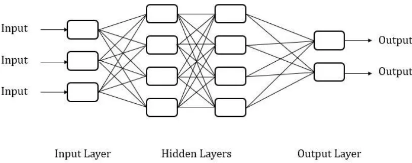
input layer, one or more hidden layers, and output layer (see Figure 1). The input layer is where

data is fed at the beginning of the training process and anytime the network is used to predict

(20)

occur and it has neurons, connections of weights and biases, propagation function, and a learning

rule. Neurons in the hidden layer are trained where only one neuron is activated for each input. This

is achieved through forward or backward propagation where neurons are assigned weights after

comparing the input to the output value and calculating the gradient of the loss function. The output

layer contains the final form of the input data after it is processed. ANNs are widely used in

different applications such as: pattern recognition, classification, regression, and clustering.

Figure 1. TypicalArtificial Neural Network structure.

ANNs have advantages over the conventional models in demand forecasting applications. ANNs

can generalize and model nonlinear complex relationships. That is important because most real-life

problems have a nonlinear and complex relationship between inputs and outputs. In addition, ANNs

have a high computational capacity, the ability to generalize, and infer unseen relationships on

unseen data. Researchers (Adamowski & Karapataki 2010, Ghiassi et al. 2008; Jain & Ormsbee

2002) have used ANNs in short-term water demand forecasting application and showed that ANNs

outperforms traditional forecasting technique. In this study, four ANN models are deployed to

forecast the water demand t-time steps ahead. Then, these models are compared to a traditional

adequate forecasting model based on two criteria: model forecasting accuracy, and computational

load.

Forecasting methodology

The focus of this study is on short-term water demand forecasting. Here, short-term refers to how

many t-time steps are forecasted ahead. Proposed models produced 8-hour, 24-hour, and 7-day

(21)

Two forecasting methodologies are presented in this study. The first methodology is the nonlinear

autoregressive with and without exogenous parameters. This group of models is investigated in

chapter 3. The second methodology, studied in chapter 4, is a hybrid model resulted from the fusion

of regression trees and self-organizing maps.

Nonlinear Autoregressive Models

Because of the seemingly nonlinear relationship in the water demand data, this nonlinear

ANN model was chosen for forecasting. Nonlinear Autoregressive (NAR) and Nonlinear

Autoregressive with Exogenous inputs (NARX) are a supervised machine learning Multi-Layer

Perceptron (MLP) feedforward ANN models. Theses two models use historical time series data to

predict in the future. The difference between NAR and NARX is that NARX utilizes more than a

single input time series to predict a target series. In this thesis, for example, NARX used the

historical water demand and weather parameters to predict the future water demand. Meanwhile,

NAR only used the historical water demand to predict the future water demand. Both models have

a similar workflow of training, testing, and validating. Both models were also built using the same

Guide User Interface (GUI) neural net time series package in MATLAB R2017b platform.

Processed data is loaded to the workplace. Then, target data and input data are selected to be fed to

the network input layer. At this step, the time series format is selected where data is converted into

a standard neural network cell array form. The formatting function chosen in this study was

“tonndata” because of its compatibility with neural networks. After conversion, data is divided up

into three categories: training data, validation data, and testing data. Training data is the group

presented to the network during training step and the network will adjust based on its errors and

weights. Validation data is the portion that is used to measure the network generalization. Network

will stop training when no generalization improvement is measured. Testing data is the last portion

that is used to measure the network performance. In this study, default recommended data division

of 70% training, 15% validation, and 15% testing was used. Ideally, datasets are divided into

training dataset to build the model, and testing dataset to evaluate the model performance. However,

a validation dataset is used in ANN models to avoid overfitting issue. Overfitting occurs when the

model is excessively trained and its accuracy reaches 100%. Overfitted models are not preferred

due to their poor performance on unseen data. The validation held back dataset estimates the model

parameters independently from the training dataset.

At this step, the input layer is fully developed. Next, “narnet” or “narxnet” is used to define the

(22)

number, the hidden neurons number, and the training algorithm. Both NAR and NARX models

were first trained with the default feedback delays of 2, hidden neurons of 10, and

Levenberg-Marquardt “trainlm” as training algorithm. Levenberg-Levenberg-Marquardt is an iterative technique that

locates the minimum of a multivariate function that is expressed as the sum of squares of nonlinear

real-valued function (Levenberg, 1944). This regularization algorithm is developed to solve the

overfitting problem in ANN models. The selection of this algorithm is based on obtaining the

lowest mean squared error possible (Hagan et. al., 1995). The training algorithm, the number of

delays, and hidden neurons were adjusted based on the network performance. After the network

architecture is defined, performance measures are selected to evaluate the network. The Mean

Absolute Percentage Error (MAPE) and Root Mean Squared Error (RMSE) were selected for

performance evaluation (i.e. equations 1 & 2, respectively). In case the network performance was

not satisfactory, parameters such as number of neurons, number of delays, training algorithm, and

network retrain option, could be calibrated. After reaching a steady state, where performance does

not change with changing parameters, the closed-loop network could be exported and used to

forecast water demand.

𝑀𝐴𝑃𝐸 =1 𝑛∑ |

Yi − Ŷi Yi |

𝑛

𝑖=1

(1)

𝑅𝑀𝑆𝐸 = √1 𝑛∑(

𝑛

𝑖=1

𝑌̂𝑖 2

− 𝑌_𝑖2₎ ₍₂₎

Where,

n = the number of data points; Yi and Ŷi represent and and water outflow

i = the data point number (i.e. 1, 2, …, n)

Yi = the actual water outflow

Ŷi = the forecasted water outflow

Hybrid Model

A supervised machine learning technique is fused with an unsupervised machine learning

(23)

machine learning where no target values are known. Regression Trees (RT) technique was selected

for the supervised machine learning part. RT implicitly perform feature selection which reduces

data dimension (Breiman et al., 1984). This feature is important in a predictive model because it

minimizes irrelevant data noise, which improves the model performance and reduces time of

training. Other advantages of the RT technique are the minimal effort in data preparation, and the

ease of model interpretability. Self-Organizing Map (SOM) is a clustering unsupervised model

fused with RT technique to further reduce the data space where forecasting is performed. SOM

groups input data into a defined number of clusters based on specific similarities (Kohonen T.,

1982). In this study, the similarity criterion is set as the water demand intensity. This clustering

technique is performed before data is fed to the forecasting model, RT model. Again, both models

were built using the Guide User Interface (GUI) neural net time series package in MATLAB

R2017b platform.

First, the SOM model is built, trained, validated, and tested. Input data is selected in matrix form

within the neural clustering tool (nctool). After input data is loaded, the SOM network architecture

is defined where clustering function and number of neurons are selected. In this study,

“selforgmap” function is used to define the: row vector dimension size, number of training steps,

initial neighborhood size, layer topology function, and neuron distance function. Values of these

parameters were initiated as the tool recommended default (i.e. 2 neurons, 100 training steps, 3

neighborhood size, hexa-topology, “linkdist”). These parameters could be replaced by different

values; however, the number of neurons was the dominant parameter that affected the SOM

performance. Next, SOM is trained using the batch unsupervised weight/bias algorithm. Weights

and biases are calculated and updated at the end of the entire pass of input data. The output of SOM

is binary determining if an instance belongs to a specific cluster or it does not.

Second, SOM cluster number is added to the input data and uploaded to the RT model workplace.

RT model requires defining the parameters of: number of cross-validation folds, maximum number

of splits and minimum leaf size, Principal Component Analysis (PCA) feature, and the fitting

algorithm.

• Cross-validation folds: It is important to define and include this feature to prevent the

common training issue, overfitting. Number of folds was initially chosen to be 5 (default).

• Maximum number of splits and Minimum leaf size: RT algorithms grow deep trees by

default, determining the number of maximum splits and leaf size helps in reducing model

complexity and training time. The number of maximum splits and minimum leaf size

(24)

• Principal Component Analysis (PCA): this feature was enabled to transform features and

remove redundant dimensions. PCA prevents the model from learning a previous learnt

information. PCA extracts a small number of variables that best explain variance in the

dataset.

• “fitrtree”: this was the algorithm used to fit the RT model. “fitrtree” returns a regression

tree based on the input value contained in the predictor matrix and the output value in the

response matrix.

After defining and selecting the previous parameters, RT model is trained, and performance is

calculated. Further modifications are applied if the performance is unsatisfactory. This includes:

adding extra neurons in the SOM model, add folds, increase the maximum splits and minimum leaf

size values in the RT model.

References

Adamowski, J. & Karapataki, C., 2010. Comparison of multivariate regression and artificial neural

networks for peak urban water-demand forecasting: Evaluation of different ANN learning

algorithms. Journal of Hydrologic Engineering, 15(10), 729–743.

Breiman L., 1984. Classification and Regression Trees. Belmont, CA: Wadsworth International

group.

Ghiassi, G., Zimbra, D.K., Saidane, H., 2008. Urban water demand forecasting with a dynamic

artificial neural network model. Journal of Water Resources Planning and Management

134 (2), 138-146.

Hegan M. T., Demuth H. B., Beale M., 1995. Neural Network Design. Boston: PWS-.

Jain, A. & Ormsbee, L., 2002. Short-term Water demand forecast modeling techniques —

Conventional Methods versus AI. Journal American Water Works Association, 94(7), 64–

72.

Kohonen T., 1982. Clustering, Taxonomy, and Topological Maps of Patterns. Proceedings of the

6th International Conference on Pattern Recognition.

Levenberg K., 1944. A Method for the Solution of Certain Non-Linear problems in Least Squares.

Quarterly of Applied Mathematics, 2, 164-168.

Rice, D.C.J., Carriveau, R., Ting, D.S.-K. & Bata, M. H., 2017. "Evaluation of Crop to Crop Water

(25)

CHAPTER 3 Short-term Water Demand Forecasting Using Nonlinear Autoregressive Artificial Neural

Networks (ANN)

Mo’tamad H. Bata, Rupp Carriveau, and David S.-K. Ting

Turbulence and Energy Laboratory, Ed Lumley Centre for Engineering Innovation, University of Windsor,

Windsor, ON N9B 3P4, Canada.

Nomenclature

The following symbols are used in this chapter:

ANN = Artificial neural network

NARX = Non-linear autoregressive with exogenous inputs model

NAR = Non-linear autoregressive model

SARIMA = Seasonal Autoregressive Integrated Moving Average

MAPE = Mean absolute percentage error

NRMSE = Normalized root mean squared error

m3 _{= Cubic meter}

hr = Hour

HD = Hot Deck

o

C = Degree Centigrade

g = Gram

W/m2 = Watt per squared meter

kPa = Kilo Pascal

PCC = Pearson Correlation Coefficient

MLP = Multi-layer perceptron

ARX = Autoregressive with exogenous inputs model

𝑌𝑖 = Current observed value of time series

Xi = Current value of exogenous time series

t = Time

n = Number of data point (i.e. 1, 2, 3, etc.)

RMSE = Root mean squared error

𝑌

̅

𝑖 = Data set mean

(26)

Introduction

Providing reliable, secure potable water to consumers is a vital core aspect of any water utility’s

daily operations. Short-term water demand forecasting can help a water utility to more efficiently

manage many of their principal operations. These include the distribution system, pumping

schedule, and storage assets. Water demand is temporally and spatially dynamical, often in short

time frames. Water demand profiles are very dependent on regional influences. Some of the main

driving factors are consumer type, water prices, population growth, economic growth,

technological practices, and management strategies. A forecasting model’s capacity to take into

consideration the aforementioned variables is important; three main factors are deemed the main

engine of a relatively accurate model. The first and most important factor is the input. Researchers

(Guo et al., 2018; Arandia et al., 2016; Alvisi et al., 2007; Homwongs et al., 1994; Shvartser et al.,

1993; Jowitt and Chengchao, 1992) have used historical water demand as a single input in their

forecasting models. Their models showed reasonably accurate forecasts. Others (Rice et al., 2017;

Herrera et al., 2010; Ghiassi et al., 2008; Bougadis et al., 2005; Aly and Wankule, 2004; Jain and

Ormsbee, 2001; Jain et al., 2001) have used extra (Exogenous) inputs in addition to the historical

water demand, weather and seasonality data, such as, temperature, rainfall, and evaporation, time

of the day, and day of the week. The inputs used in this study are explained in the Methods section.

The second driving factor is the time horizon, which contains two-time dimensions, one to

determine how far back the historical data is needed, and one to set the length of the forecast.

Previous studies have chosen the historical time span without clarifying the reasons for selection.

In this paper, historical hourly data of the last 5 years (2013-2017), the most recent year of the 5

years data (2017), and the 4 most recent months of the most recent year (September 2017-December

2017) were used as inputs. These were chosen to investigate the effects of historical data length

on the forecast accuracy. The other time dimension is how far ahead the model will forecast, this

horizon is governed by the model application (Bakker et al., 2003). Short-, medium-, and long-term

forecast horizons have been extensively discussed by (Donkor et al., 2012; Billings and Jones 2008;

Gardiner and Herrington 1990). For our purposes here, short-term forecast horizons of 24 hours

and 1 week ahead were utilized for the purpose of daily operations and pumping schedule control.

The third significant factor is the model method itself. Many studies have assumed the presence of

(27)

progressively learn, self-train, and improve performance of demand forecasting systems. They have

been broadly used in demand forecasting in various applications. Kandananond, 2011; Chang et

al., 2011; Feilat & Bouzguenda, 2011; Amjady & Keynia, 2011; Azadeh et al., 2007 used ANN in

electricity load forecasting. Guo et al., 2018; Bennet et al., 2013; Adamowski & Karapataki, 2010;

Mitrea et al., 2009; Ghiassi et al., 2008; Jain & Ormsbee, 2002 used ANN in water demand

forecasting and showed that it outperformed traditional water demand forecasting techniques.

Although many ANN approaches have proven useful in modeling complex demand forecasting, a

few undetermined parameters of the model architecture have made ANN models harder to elucidate

and optimize. Theses architectural parameters include the training algorithm, and the optimal

number of neurons and hidden layers.

Guo et al., 2018 broadly classified water demand forecasting methods into traditional methods and

learning algorithms. Traditional statistical methods have used linear time series or linear regression

to tackle this challenge and have proposed simple statistical models (Wong et al., 2010; Zhou et

al., 2000) to tackle it. A popular model used extensively among this group is the Autoregressive

Integrated Moving Average (ARIMA). These models have been widely used (Kofinas et al., 2014)

because they have a simple structure, are easy to implement and interpret, and do not require a lot

of input data. Learning algorithms identify water demand forecasting as a nonlinear problem. With

the progressive advancements in machine learning and data analytics, these algorithms have

achieved higher accuracy in prediction models. Support Vector Machine (SVM), Artificial Neural

Networks (ANN) and Deep Learning models are the most studied within this group. More detailed

description and the use of traditional methods and learning algorithms can be found in Arandia et

al., 2016 and Guo et al., 2018.

In this manuscript, two nonlinear ANN models and one linear ARIMA model were employed with

a specific architecture to forecast water demand. Model nature and methodology (i.e. linear vs.

nonlinear) was first investigated. Secondly, input type (single input vs. exogenous inputs) influence

on the predicting model was studied. Lastly, data size was scrutinized in an attempt to determine

how far back the data is required to be.

Study Area and Data

Union Water Supply System (UWSS) is a municipal water supply system owned by the Ontario

municipalities of Leamington, Kingsville, Essex, and Lakeshore. UWSS supplies water to

approximately 65,000 residents and in addition to commercial, industrial and agricultural

(28)

utility’s outflow is consumed by commercial greenhouses. The rest, 22%, is consumed by the

residential and industrial sectors.

Five years (Jan 2013 – Dec 2017) of continuous hourly data was used to train the models. It was

grouped into three main categories, the plant outflow measured in m3_{/hr (see Figure 1), the weather,}

and the seasonality. Outflow data had 3.75% of missing and erroneous (i.e. zero data) data, missing

data was imputed using the Hot Deck (HD) method, and the imputation was based on the highest

correlated factor, previous day same hour, shown in Table 1. Further description of the imputation

is discussed in the Data Pre-processing section.

Figure 1. Utility water outflow m3_/hr

The observed weather data at t=0 is used as an exogenous input in the proposed NARX models to

predict at t=24 and t=168; hourly data of ambient temperature (0_{C) (see Figure 2), dew point (}0_C),

absolute humidity (g H2O / m3 air), solar radiation (W/m2), and station pressure (kPa). A total of

2.30% missing data, mainly solar radiation, was imputed similarly using the HD method. The last

category is the seasonality and it contains the year (2013-2017), the month (1-12; 1 represents

January and 12 represents December), the day of the month (1-28,29,30 or 31), the day of the week

(1-7; 1 represents Saturday and 7 represents Friday), and hour of the day (1-24; 1 represents 12:00

(29)

Figure 2. Ambient temperature (0_C)

In terms of input data, the Pearson Correlation Coefficient (PCC, also referred to as Pearson’s r) is

evaluated for 14 different demand, weather, and seasonality predictors. The 14 input predictors

were selected according to data availability and previous consideration in demand forecasting

literature. In Table 1, the predictors PCC is shown in one column and the correlation strength is

shown in the other column. The correlation strength is a description using the guide proposed by

(Evans, 1996) for the absolute value of r. PCC ranges between 1 and -1,where 1 is the total positive

linear correlation, 0 is no linear correlation, and −1 is the total negative linear correlation. While

PCC is not robust in terms of measuring dependency (Wilcox, 2005), other robust estimators of

correlation are not as interpretable as PCC.

Table 1. PCC measured for the predictors

Predictor Rank PCC Strength

Previous day same hour 1 0.835 Very strong

Previous week same hour 2 0.758 Strong

Previous 24hrs average 3 0.569 Moderate

Temperature 4 0.478 Moderate

Absolute humidity 5 0.397 Weak

Dew point 6 0.393 Weak

Solar radiation 7 0.363 Weak

(30)

Month 9 0.036 Very weak

Hour of the year 10 0.035 Very weak

Hour of the day 11 0.026 Very weak

Day of the week 12 0.020 Very weak

Station pressure 13 - 0.010 Very weak

Day of the month 14 0.007 Very weak

Data Pre-processing

Missing data is an untold story of a record. Missing data is a common occurring issue that

significantly affects the information that can be drawn from the data. The missingness could be a

result of many reasons. Some of these common reasons are: incomplete data collection, faulty

equipment, non-response in data, and impractical feature case.

Handling missing data is essential prior to deploying it. Missing data could be discarded; this is the

simplest technique of handling the missingness. However, it is not effective if the missingness rate

is high. Also, missing data could be replaced, estimated, or filled based on domain knowledge

(Salvador et al. 2015). In this paper, missing data is handled by imputation, where the missing

values are filled to form a complete dataset. One used popular strategy of imputation is the Hot

Deck.

The term “Hot Deck” originally used as computer punch cards for data storage, and refers to the

deck of cards for donors available for a non-respondent. The deck was “hot” since it was currently

being processed, as opposed to the “cold deck” which refers to using pre-processed data as the

donors, i.e. data from a previous data collection or a different data set (Andridge et al. 2010).

Hot Deck is a common imputation technique and is considered in this paper. With HD imputation,

the missing value is replaced by a similar responding unit. This method is extensively used in

practice where a non-respondent missing value (called the recipient) is replaced by a respondent

value (called the donor) with respect to characteristics observed by both cases (Andridge et al.

2010). Selection of the donor leads to two versions of the Hot Deck imputation. The first version

is the Random Hot Deck method where the donor is selected randomly from a donor pool. Whereas

for the second version, the Deterministic Hot Deck, one single donor is selected; usually the nearest

neighbor.

(31)

is equal one. The nearest neighbor is determined though a distance function, herein, the Euclidean

Distance presented in equation 1.

𝑑 = √∑𝑛 (𝑄𝑖 − 𝑃𝑖)2

𝑖=1 (1)

Where,

d is the Euclidean Distance

i is the record number

n is the dimension number

Q is the reference point

P is the target point

The methodology of the HD imputation is simple. If Y and X are two variables/features where Y is

the target (i.e. the Donee) column that has the missing values and X is the covariant (i.e. the Donor).

For the missing value Y4, the distance function (i.e. Euclidean Distance) determines the nearest

neighbor to X4. Then, the corresponding Yn of that nearest Xn is replaced for the original missed

value, Y. Figure 3 illustrates the process.

Figure 3. Nearest Neighbour Hot Deck Imputation

Methods and Model development

SARIMA Model

SARIMA is a simple statistical model that is used to analyze and predict a time series.

SARIMA is a seasonal generalization of the Autoregressive Moving Average (ARMA) with the

(32)

parameters and are denoted by ARIMA (p, d, q) x (P, D, Q)S(Shumway and Stoffer, 2000). The (p,

d, q) non-seasonal order of the model is the number of Autoregressive (AR) parameters,

differences, and Moving Average (MA) parameters. The (P, D, Q)Sorder of the seasonal component

of the model is the AR parameters, differences, MA parameters, and periodicity. These

non-seasonal and non-seasonal parameters are iteratively identified through plotting the Autocorrelation

Function (ACF) and the Partial Autocorrelation Function (PACF). Regarding the data needed to

properly fit a SARIMA model, Arandia et al., 2016, showed that a 7-day window is enough to

forecast 24 hours ahead. In this paper, two SARIMA models with two different training windows

were fitted to forecast water demand. The first model, ARIMA (0, 1, 1) X (0, 1, 1)24, used 7 day

hourly water demand data to forecast 24 hours ahead. The second model, ARIMA (0, 1, 1) X (0, 1,

1)168, used four recent months of hourly water demand data to forecast 7 days ahead.

Nonlinear Autoregressive with Exogenous inputs (NARX)

NARX models are recurrent dynamic networks with feedback connections that enclose

several layers of the network. NARX is a Multi-Layer Perceptron (MLP) feedforward ANN. These

models are based on the linear ARX model, which is commonly used in time-series modeling.

(Pisoni et al., 2009) claimed that the nonlinear neural network models (NARX) have better

performance than the polynomial NARX models. Later (Mustafaraj et al., 2011) validated that

claim and showed that neural network NARX models outperform the linear ARX models. A NARX

model delineates the current value of a time series (Yi) to both past values of the time series (Yi-1,

Yi-2,…, Yi-n) and current (Xai, Xbi,…, Xni). It also demarcates past values of the correlated

(Exogenous) series (Xai-1, Xbi-1, …, Xni-1, Xai-2, Xbi-2, …, Xni-2, Xai-n, Xbi-n, …, Xni-n). Equation 2

illustrates the defining equation by (Demuth et al., 1998) for the NARX model and the NAR model

explained in the next section.

Y(t) = f (Yt-1, Yt-2, …, Yt-n, Xt-1, Xt-2, …, Xt-n) (2)

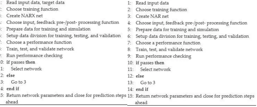
Figure 4 (a) illustrates the algorithm used to develop NARX models in the MATLAB R2017b

platform. First, data is divided into input data (Exogenous data) and its corresponding target data

(water outflow data). Then, a training function is selected based on memory performance and

problem type. Input delays, feedback delays, and hidden layer size are then estimated and the

(33)

feed a new network design at each time step. Also, at each time step, data samples are divided

randomly into training, testing, and validation. At this point, the network is ready to be trained,

however, its performance is not yet evaluated. Therefore, one or more performance functions are

selected to check whether the network performs as desired or the network parameters and structure

need to be estimated again. If the desired performance is met, network parameters are returned, and

the network is enclosed to forecast steps ahead. All NARX and NAR networks in this paper are

MLP with the same training, processing, preparing functions (i.e. trainbr, proccessfncs, and

preparets, respectively).

Three NARX models were built to forecast the water demand 24 hours and one week ahead. The

criterion that was considered to differentiate between the three models is the historical data span

length (5 years, 1 recent year, and 4 recent months) for both water outflow and exogenous inputs.

The selection of 5 years was based on the use of all available data. Meanwhile, 1 recent year and 4

recent months were selected to investigate how using less data would impact model accuracy versus

model complexity. Further selections could be made. However, the consumer activity periodicity

must be acknowledged, here that’s commercial greenhouses. A researcher could have different data

span length according to the utility consumer breakdown, for this specific utility, the division into

three main seasons was assumed to accommodate the main consumer (Commercial greenhouses)

seasons of planting.

(34)

Nonlinear Autoregressive (NAR)

NAR models are recurrent dynamic networks with feedback connections enclosing several

layers of network. NAR also is a Multi-Layer Perceptron (MLP) feedforward ANN. NAR models

are used extensively in time series demand forecasting, a comprehensive literature review by

(Moreno- Chaparro et al., 2011) lists different types of time series and methods that used NAR

models for prediction in various applications. A NAR model predicts the current value of a time

series (Yi) using past values (Yi-1, Yi-2,…, Yi-n), see Equation 3 for the defining equation. NAR

models were developed with an algorithm (see Figure 4 (b)) similar to the NARX’s. However,

NAR models are fed with only input data. Three NAR models were built in this study and used to

forecast the water demand for 24 hours and one week ahead; the same criterion used to produce the

three NARX models was used similarly in the NAR models.

Y(t) = f (Yt-1, Yt-2, …, Yt-n) (3)

Baseline comparison and model performance

The actual measured water outflow is used as a basis for evaluation. The forecasted target value

(Ŷi) is compared to the target actual measured value (Yi) and overall model performance is

measured by: (1) Mean Absolute Percentage Error (MAPE) and (2) Root Mean Squared Error

(RMSE). However, the dataset that was used as an input for the models has different ranges and

means, the Normalized Root Mean Squared Error (NRMSE) is included to syncretize those

differences. Equations 4, 5 and 6 represent the MAPE, RMSE and NRMSE, respectively, where n

represents the number of data points; Yi and Ŷi represent the actual and the forecasted and water

outflow, respectively, and 𝑌̅𝑖 is the data set mean.

𝑀𝐴𝑃𝐸 =1 𝑛∑ |

Yi − Ŷi Yi |

𝑛

𝑖=1

(4)

𝑅𝑀𝑆𝐸 = √1 𝑛∑(

𝑛

𝑖=1

𝑌̂𝑖 2

(35)

𝑁𝑅𝑀𝑆𝐸 =𝑅𝑀𝑆𝐸 𝑌̅𝑖

(6)

Results and Discussion

Linear vs. Nonlinear

The results for the seven proposed models forecasting 24 hours ahead and 1 week ahead

are shown in Table 2. It can be observed that the forecast in both time horizons have a relatively

better overall performance when nonlinear models (i.e. NAR and NARX) were employed

compared to the linear models (i.e. SARIMA). On average, MAPE error for NAR models compared

to the SARIMA models is 3% and 15% less, forecasting 24 hours ahead and 1 week ahead,

respectively. Likewise, NARX models performed with 30% and 36% less error compared to

SARIMA models, forecasting 24 hours ahead and 1 week ahead, respectively. That is because of:

(1) nonlinear models are able to capture both linearity and nonlinearity in the time series; and (2)

nonlinear models employed in this paper, ANN models, have a complex multi-layer structure that

finds correlation between input, feedback, and output parameters. Regarding model stability,

nonlinear models seem to perform with greater stability as the relative error values are lower

compared to linear models.

Table 2. Models overall performance

MAPE (%)

NRMSE (%)

Relative Error

Forecast ahead Historical data Model Standard

deviation

Percentile

5% 95%

2 4 Ho u rs

7 days SARIMA-24 17.5 17.7 0.0821 ±0.86% ±9.65%

5 years NAR-5y 18.6 18.9 0.0873 ±0.78% ±9.16%

1 year NAR-1y 17.5 17.6 0.0816 ±0.75% ±8.48%

4 recent months NAR-4m 14.8 15.2 0.0701 ±0.72% ±8.62%

5 years NARX-5y 18.1 18.5 0.0864 ±0.64% ±7.95%

1 year NARX-1y 13.4 13.6 0.0622 ±0.46% ±6.80%

4 recent months NARX-4m 04.3 06.6 0.0438 ±0.23% ±5.78%

7

Day

s

4 recent months SARIMA-168 19.7 22.6 0.0934 ±0.79% ±11.55%

5 years NAR-5y 19.1 20.2 0.0898 ±0.74% ±10.84%

1 year NAR-1y 18.7 19.2 0.0904 ±0.83% ±9.98%

(36)

5 years NARX-5y 18.5 18.7 0.0868 ±0.69% ±10.45%

1 year NARX-1y 13.6 13.9 0.0703 ±0.57% ±7.12%

4 recent months NARX-4m 05.6 07.0 0.0486 ±0.16% ±6.14%

Single Input vs. Exogenous inputs

Another perspective that affected model performance was the input type. Here, the

proposed models are grouped into single input models, and exogenous models (i.e. models that

have X in their identifier name). SARIMA models and NAR models belong to the first group by

feeding only the water outflow as a model input. Whereas, NARX models have been fed by extra

correlated weather inputs. NARX average overall performance in terms of error, MAPE, decreased

by 30% and 25% compared to NAR models forecasting 24 hours ahead and 1 week ahead,

respectively. NARX average error also decreased, as mentioned before, by 30% and 36% compared

to SARIMA models. Even though NAR and NARX models have a similar structure, the inclusion

of exogenous parameters has advantaged the ANN model. Again, this is due to extra correlations

drawn from the extra inputs. In addition, NARX models have lower relative error, which may

suggest greater stability.

Data span

Data span here refers to how far back data is needed to adequately train a model. The data

span focus in this research was on the ANN models. Results show that four months data was

sufficient to train both NAR and NARX models. Comparing 4 months to 5 years and 1 year data

models, error dropped by 20% and 15% in NAR model and by 76% and 68% in NARX model,

respectively, forecasting 24 hours ahead. Further, there were reductions by 35% and 33% in NAR

model and by 70% and 59% in NARX model, respectively, forecasting 1 week ahead. While it may

be intuitive to expect that a time series model would improve with more historical data; this was

not the case in this research. Both NAR and NARX models had a drastic error decrease when fed

with less historical data. The reason is due to the data itself rather than the model structure. A major

change in water consumption profiles had occurred in the region where the utility is located.

Greenhouses, the main consumer, started to switch from growing vegetables to Marijuana after the

new Canadian legalization act occurred in 2018. The change in agricultural activities in the studied

area had affected water demand profiles and left the historical data with little information to add.

(37)

model. These exogenous parameters reinforced the model by adding more information when the

studied parameter (i.e. water outflow) no longer had the same trend, seasonality, and consumption

profiles.

Computational Load

As mentioned earlier, SARIMA models have a simple structure and do not require a large

quantity of data for training. On the other hand, NAR models have a complex structure and use

more parameters. Even more complicated, NARX models are fed with exogenous inputs. This

increases the model complexity and number of parameters. Model performance indicators are a

good measure for model accuracy. However, they do not necessarily embody the model complexity

issue. Therefore, the computational load was evaluated to better reflect the model’s complexity and

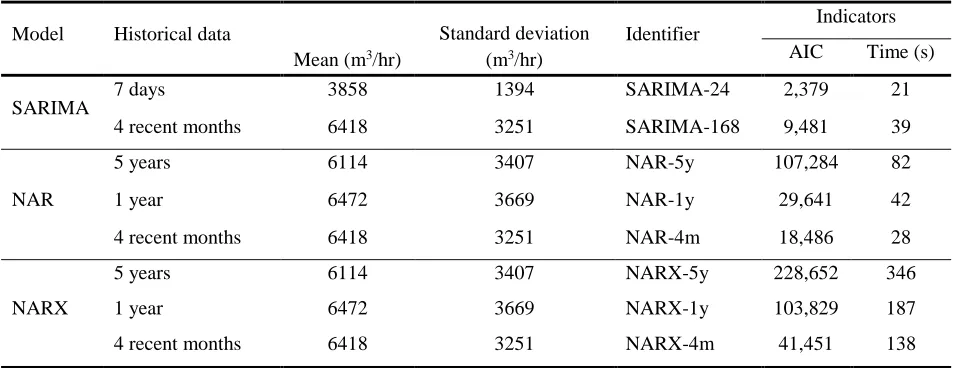
deployment practicality. Computational load, Table 3 was evaluated from two perspectives: (1)

Akaike Information Criteria (AIC), which penalizes models that use more parameters; and (2)

Computation time spent during data training steps. The computational tool used in this research

was HP Pavilion TS 14 Notebook PC with a 1.6 GHz Intel Core i5 processor and 8 GB memory.

Table 3. Computation load of forecasting models on training data

Model Historical data

Mean (m3_/hr)

Standard deviation (m3_/hr)

Identifier Indicators

AIC Time (s)

SARIMA

7 days 3858 1394 SARIMA-24 2,379 21

4 recent months 6418 3251 SARIMA-168 9,481 39

NAR

5 years 6114 3407 NAR-5y 107,284 82

1 year 6472 3669 NAR-1y 29,641 42

4 recent months 6418 3251 NAR-4m 18,486 28

NARX

5 years 6114 3407 NARX-5y 228,652 346

1 year 6472 3669 NARX-1y 103,829 187

4 recent months 6418 3251 NARX-4m 41,451 138

AIC and training time results reveal that the SARIMA model had the lowest and most preferred

performance. SARIMA-24 has had a relatively low AIC due to the shortest data span, 7 days, used

to feed the model. SARIMA-168 with a similar structure had a 4-fold higher AIC. This was because

the model was trained with a longer data span, 4 recent months. Ranked second was the NAR

model. The ANN single input model with complex structure had approximately twice the AIC over

(38)

with the same four recent months data. Lastly, for the ANN model with exogenous inputs, the

NARX-4m showed an AIC 4-times higher than the SARIMA-168, and 2-times higher than the

NAR-4m. This ranking was anticipated because AIC consists of two terms, likelihood and number

of parameters. Table 3 and Figure 5 show that the number of parameters was the dominant

determinant in AIC values. Exogenous inputs along with longer data span added more parameters

and errors to their associated models.

Figure 5. Datasets distribution and outliers.

Model Error Histogram

The error histogram for one of the proposed models, specifically, NARX-4m, is shown in Figure

6. For a forecast of 24 hours ahead with a mean of 5852m3_{/hr, the model predicted roughly 35.50%}

of the data with an overestimation average of 38.9 m3_{/hr. Also, 20.15% and 24.34% of the data}

were overestimated and underestimated by an average of 461m3_{/hr and 447m}3_{/hr, respectively. In}

total, approximately 80% of the 2238 predicted hours were estimated with an error of less than 10%

of the mean. That said, approximately 5%, 110 hours of the 2238 hours tested to forecast 24 hours

ahead, had an overestimation or underestimation by 1000-2000 m3_{/hr. This relatively high error in}

forecasting is deemed to be due the dramatic peak during some random mid-day hours. This drastic

change in the outflow was not tracked by the one-hour data models. A shorter time span dataset,

e.g. 15 minutes, would have decreased the percentage and amount of overestimation or

(39)

Figure 6. NARX-4m model error histogram

Models application

In this section, one week (12/02/2107 3:00pm – 12/09/2017 2:00pm) water outflow data

was extracted from the utility daily operational data log and held back. SARIMA, NAR, and NARX

models were deployed to forecast the water outflow for 24 hours ahead and 1 week ahead. The

results of the performance in terms of MAPE are shown in Table 4. In addition, the forecasted

patterns were compared to the actual held back water outflow for the targeted time horizon, Figures

7 and 8 display the results for models forecasting 24 hours ahead and 1 week ahead, respectively.

Both results forecasting 24 hours ahead and 1 week ahead show a better performance for nonlinear

models (i.e. NAR and NARX) over linear (i.e. SARIMA) models. Also, the models with exogenous

parameters have outperformed the models with single input. Furthermore, shorter data span models,

4m, performed better than models with longer data span, 5y and 1y.

Table 4. Deployed models performance

Forecast ahead Model Error (%)

MAPE NRMSE

24 H

our

s

SARIMA-24 17.9 18.3

NAR-5y 15.6 15.9

NAR-1y 16.5 16.5

NAR-4m 13.8 13.5

NARX-5y 14.1 14.0

(40)

NARX-4m 12.3 12.7

7 D

ays

SARIMA-168 19.7 19.4

NAR-5y 16.1 16.3

NAR-1y 15.7 15.4

NAR-4m 14.4 14.6

NARX-5y 16.5 16.1

NARX-1y 13.1 13.3

NARX-4m 10.6 11.0

Figure 7. Models forecasting water demand 24 hours ahead (12/02/2107 3:00pm – 12/03/2017