XU, DEZHONG. Development and Testing a New Ramp Weave Operational Analysis Method. (Under the direction of Dr. Nagui Rouphail).
In the past several decades, the methodology of the Highway Capacity Manual (HCM)
weaving segments has been updated several times. In the latest version, HCM6, the method
predicts the speed of weaving and non-weaving traffic by using the predicted number of lane
changes. However, recent research has revealed that the speed and capacity prediction of HCM6
is not accurate and lacks sensitivity to important design parameters under certain conditions.
The goals of this study are to provide a simple method for ramp weave segments and to
ensure consistency with other freeway segment analyses in HCM6. It includes a new modeling
framework that maintains a continuum between the operation of the weaving segments to an
equivalent basic segment that has a similar volume, number of lanes, and free-flow speed. This
study focused on ramp weaves only. The proposed models were calibrated using data from seven
mostly local sites, including one site from NCHRP 3-75 and six additional sites with data
gathered from ground-based and drone videos. Several methods were tested for data reduction,
including image processing and manual extraction. The calibrated models were assessed using
several numerical sensitivity tests.
Based on the results of the tests, it is shown that the proposed approach is practical and
accurate. The proposed models are proven to have better goodness of fit to observed speeds than
HCM6, explaining about 75% of the variability in observed 5 min- mean speeds. The models’
sensitivities of speed and capacity to segment length, volume ratio, and demand are reasonable
© Copyright 2019 by Dezhong Xu
by Dezhong Xu
A thesis submitted to the Graduate Faculty of North Carolina State University
in partial fulfillment of the requirements for the degree of Master of Science of Engineering
Civil Engineering
Raleigh, North Carolina 2019
APPROVED BY:
_______________________________ _______________________________ Nagui Rouphail Billy Williams
Committee Chair
_______________________________
DEDICATION
First, I would like to express the deepest appreciation to my committee chair, Dr. Nagui
Rouphail, who gave me the opportunity and guided me through the main research project. I
would never be able to accomplish anything without his support.
I would also like to thank my parents, who have always supported me. Their care and trust
supported me in getting out of the depression and gaining the strength to face the challenges.
And I would like to offer my gratitude to my beloved, Dan Yu, who has inspired me with her
love, understanding, and company.
I am further grateful to thank all my friends for their support. I thank all professors in the Civil
Engineering Department for their excellent lectures and advises.
Finally, my gratefulness also goes to my cat Marra, who always stay by my side and
BIOGRAPHY
Dezhong Xu received his B.S. degree in Civil Engineering at North Carolina State
ACKNOWLEDGMENTS
The author wishes to sincerely thank Dr. Nagui Rouphail of North Carolina State
University. He is the first individual who developed the original framework. Without his advice
and patient teaching, the completion of this study would have been extremely difficult.
Special acknowledgment is also expressed to Dr. Behzad Aghdashi of North Carolina
State University and Dr. Lily Elefteriadou at the University of Florida as they contributed to all
phases of research, especially in model development, validation and review of the Highway
Capacity Manual method.
The author expresses his greatest regards to members of the Committee on Final
Examination, Dr. Nagui Rouphail, Dr. Behzad Aghdashi, and Dr. Billy William of North
Carolina State University, for their suggestions and comments. Additionally, the author wishes to
thank the Institute of Transportation and Research for providing the facilities during research.
TABLE OF CONTENTS
LIST OF TABLES ... vi
LIST OF FIGURES ... viii
Chapter 1: Introduction ... 1
1.1 Research Objectives ... 1
1.2 Definition of Ramp Weave and Level of Service ... 2
1.3 Glossary of Terms ... 4
1.4 Thesis Organization ... 6
Chapter 2: Previous Works... 7
2.1 HCM Development History of Weaving Operational Analysis ... 7
2.2 Related Studies... 14
2.3 Works that Critically Analyzed HCM6 ... 15
Chapter 3: Methodology... 18
3.1 Scope of Work ... 18
3.2 Site Selection ... 18
3.3 Data Collection ... 20
3.4 Data Extraction ... 21
3.5 Data Filtering ... 22
3.6 Conceptual Model Formulation ... 24
3.7 Variables in SIW ... 29
Chapter 4: Model Result ... 45
4.1 Candidate Model Forms and Model Calibration ... 45
4.2 Procedure Implementation ... 69
4.3 Sensitivity Analysis to Ls ... 71
4.4 Sensitivity Analysis to VR ... 74
4.5 Sensitivity Analysis to Vrr ... 79
4.6 Limited Model Validation... 85
Chapter 5: Conclusions and Recommendations ... 89
5.1 Conclusions ... 90
5.2 Recommendations for future research ... 93
References ... 94
LIST OF TABLES
Table 1.1 Level of Service Criteria of a Weaving Segment ... 3
Table 1.2 Terminology ... 4
Table 2.1 HCM1965 Relationship Between LOS and Quality of Flow on a Weaving Section . 9 Table 2.2 Quality of Flow and Maximum Lane Service Volumes in a Weaving Section ... 10
Table 2.3 Criteria for Unconstrained vs. Constrained Operation of Weaving Areas ... 11
Table 2.4 LOS Criteria for Freeway Weaving Sections in HCM1985 ... 12
Table 2.5 HCM1985 Limitations on Weaving Area ... 12
Table 2.6 LOS Criteria in HCM1997 ... 13
Table 3.1 Location of Study Sites ... 19
Table 3.2 Summary of Configuration and Data Points of the Site ... 23
Table 3.3 Candidate Variables that Explain the Effect of Flow and Configuration to SIW .... 30
Table 4.1 Parameter Calibration Result and Goodness of Fit for Different ‘a’ Value Models ... 47
Table 4.2 Model Calibration Results and Goodness of Fit Comparison Between Candidate Models and HCM6 ... 48
Table 4.3 Two-Tailed t-test Result of the Trendline of Each Model and HCM6 (Level of Significance = 0.05) ... 61
Table 4.4 Assumed OD volumes for Different VR ... 74
Table 4.5 Assumed OD volumes for Different Percentage of Ramp to Ramp Traffic ... 79
Table 4.6 Observed OD Volumes and SMS for each 5-min period ... 85
LIST OF FIGURES
Figure 1.1 Flow Identification ... 2
Figure 1.2 Example of a Type A Weaving Segment ... 3
Figure 2.1 HCM1950 Traffic Volumes and Speed Relation Plot ... 7
Figure 2.2 Snapshot of HCM1965 Quality of Flow Curves and Relative Estimated Speeds ... 9
Figure 3.1 Image of the Drone ... 21
Figure 3.2 Graphical Illustration for Capacity and LOS Estimation ... 28
Figure 3.3 versus Normalized SMS Plot ... 32
Figure 3.4 Candidate 1 versus Normalized SMS Plot ... 33
Figure 3.5 Candidate 1 versus Normalized SMS Plot ... 33
Figure 3.6 Candidate 1 versus Normalized SMS Plot ... 34
Figure 3.7 Candidate 1 VR versus Normalized SMS Plot ... 34
Figure 3.8 Candidate 1 versus Normalized SMS Plot ... 35
Figure 3.9 Candidate 1 versus Normalized SMS Plot ... 35
Figure 3.10 Candidate 1 versus Normalized SMS Plot ... 36
Figure 3.11 Candidate 2 versus Normalized SMS Plot ... 37
Figure 3.12 Candidate 2 versus Normalized SMS Plot ... 37
Figure 3.13 Candidate 2 versus Normalized SMS Plot ... 38
Figure 3.14 Candidate 2 versus Normalized SMS Plot ... 38
Figure 3.16 Candidate 2 versus Normalized SMS Plot ... 39
Figure 3.17 Candidate 2 versus Normalized SMS Plot ... 40
Figure 3.18 Candidate 3 versus Normalized SMS Plot ... 41
Figure 3.19 Candidate 3 versus Normalized SMS Plot ... 41
Figure 3.20 Candidate 3 versus Normalized SMS Plot ... 42
Figure 3.21 Candidate 3 versus Normalized SMS Plot ... 42
Figure 3.22 Candidate 3 versus Normalized SMS Plot ... 43
Figure 3.23 Candidate 3 versus Normalized SMS Plot ... 43
Figure 3.24 Candidate 3 versus Normalized SMS Plot ... 44
Figure 4.1 Observed SMS versus Model 1 Predicted SMS Plot... 54
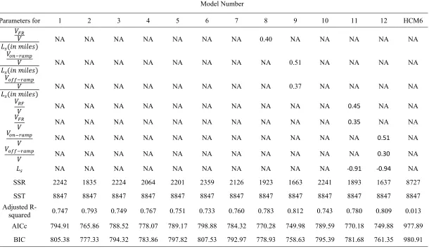
Figure 4.2 Observed SMS versus Model 2 Predicted SMS Plot... 54
Figure 4.3 Observed SMS versus Model 3 Predicted SMS Plot... 55
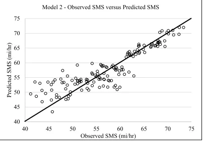
Figure 4.4 Observed SMS versus Model 4 Predicted SMS Plot... 55
Figure 4.5 Observed SMS versus Model 5 Predicted SMS Plot... 56
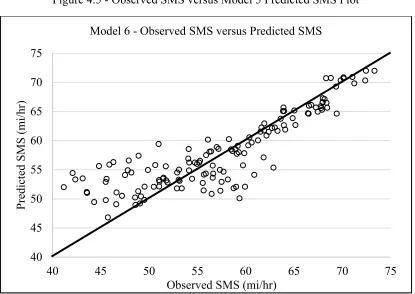
Figure 4.6 Observed SMS versus Model 6 Predicted SMS Plot... 56
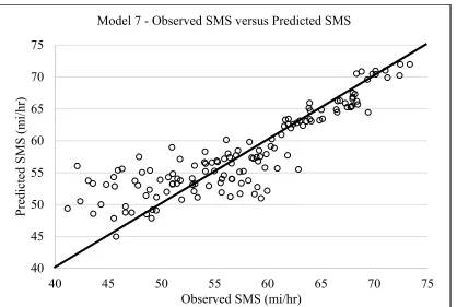
Figure 4.7 Observed SMS versus Model 7 Predicted SMS Plot... 57
Figure 4.8 Observed SMS versus Model 8 Predicted SMS Plot... 57
Figure 4.9 Observed SMS versus Model 9 Predicted SMS Plot... 58
Figure 4.11 Observed SMS versus Model 11 Predicted SMS Plot... 59
Figure 4.12 Observed SMS versus Model 12 Predicted SMS Plot... 59
Figure 4.13 Observed SMS versus HCM6 Predicted SMS Plot ... 60
Figure 4.14 Model 1 Residual Plot ... 62
Figure 4.15 Model 2 Residual Plot ... 62
Figure 4.16 Model 3 Residual Plot ... 63
Figure 4.17 Model 4 Residual Plot ... 63
Figure 4.18 Model 5 Residual Plot ... 64
Figure 4.19 Model 6 Residual Plot ... 64
Figure 4.20 Model 7 Residual Plot ... 65
Figure 4.21 Model 8 Residual Plot ... 65
Figure 4.22 Model 9 Residual Plot ... 66
Figure 4.23 Model 10 Residual Plot ... 66
Figure 4.24 Model 11 Residual Plot ... 67
Figure 4.25 Model 12 Residual Plot ... 67
Figure 4.26 HCM6 Residual Plot... 68
Figure 4.27 Implementation Procedure Flow Chart ... 70
Figure 4.28 Capacity Sensitivity to Ls ... 72
Figure 4.29 Predicted Speed Sensitivity to Ls ... 73
Figure 4.30 Density Sensitivity to Ls ... 73
Figure 4.31 Capacity Sensitivity to VR (Ls = 250 ft) ... 76
Figure 4.32 Predicted Speed Sensitivity to VR (Ls = 250 ft) ... 76
Figure 4.34 Capacity Sensitivity to VR (Ls = 2000 ft) ... 77
Figure 4.35 The result of Predicted Speed Sensitivity to VR Test (Ls = 2000 ft) ... 78
Figure 4.36 Density Sensitivity to VR Test (Ls = 2000 ft) ... 78
Figure 4.37 Capacity Sensitivity to %Vrr (Ls = 250ft) ... 81
Figure 4.38 Predicted Speed Sensitivity to %Vrr Demand (Ls = 250 ft) ... 82
Figure 4.39 Density Sensitivity to %Vrr Demand (Ls = 250 ft) ... 82
Figure 4.40 Capacity Sensitivity to %Vrr Demand (Ls = 2000 ft) ... 83
Figure 4.41 Predicted Speed Sensitivity to %Vrr Demand (Ls = 2000 ft) ... 83
Figure 4.42 Density Sensitivity to %Vrr Demand (Ls = 2000 ft) ... 84
Figure 4.43 Comparison between the Model 3 Predicted Speed and Observed Speed ... 86
Figure 4.44 Comparison between the Model 4 Predicted Speed and Observed Speed ... 87
Figure 4.45 Comparison between the Model 8 Predicted Speed and Observed Speed ... 87
Figure 4.46 Comparison between the Model 9 Predicted Speed and Observed Speed ... 88
CHAPTER 1: INTRODUCTION
With decades of development, the HCM weaving segment analysis has been revised and
updated multiple times. The development direction of the HCM weaving segment analysis can
be summarized as developing simple and non-iterative models and framework that
accommodates different types of configuration and traffic operations. Some recent projects also
attempted to develop a new weaving methodology that maintains consistency in application with
other freeway segment methods, including basic freeway and ramp junctions. The current model
and analysis framework was developed in NCHRP 3-75 (Roess, et al., 2008) and later adopted in
the 2010 HCM (Transportation Research Board, 2010). Although it was updated more recently,
some researches pointed out that both speed and capacity predictions highly deviate from field
observations. This may be caused by the lack of sufficient ramp weave site data: NCHRP 3-75
only has one feasible ramp weave site. The discordant model form also generates discontinuities
in performance estimation across different types of freeway sections. The complex and lengthy
procedure of the operational analysis has also been questioned. Also, the current method requires
extensive field calibration and speed model validation. Specific problems are introduced later in
this paper.
1.1 Research Objectives
The objective of this research is to develop a simple, non-iterative and well-calibrated
speed and capacity models and framework for ramp weave segments. The models should also
improve the sensitivities to important traffic and configuration parameters such as volume ratio
(VR) and short segment length (Ls). Another objective is to keep the consistency of predictions
with other types of freeway segments. Even though the final calibrated models only address the
model form to seamlessly transition among different types of freeway sections. The research
related information including the definition of ramp weave and level of service and all the inputs
variables used in the analysis are introduced next.
1.2 Definition of Ramp Weave and Level of Service
Weaving is the crossing of two or more uninterrupted traffic flows that have the same
direction in a limited segment length. In a simple weaving segment, traffic can be categorized
into four flows based on its origin and destination. In the four flows, freeway to freeway flow
and ramp to ramp flow are non-weaving flows. freeway to ramp flow and ramp to freeway flow
are weaving flows. Figure 1.1 below shows a summary of the flow identification.
Figure 1.1 - Flow Identification
The weaving segment has multiple configurations. Based on the number of lane change
required to finish the weaving maneuvers, the segment can be categorized into three different
types: Type A, Type B, and Type C (Transportation Research Board, National Research Council,
1985). Type A, also known as ramp weave, is the weaving segment configuration where vehicles
must make one lane change to complete weaving maneuvers. Figure 1.2 illustrates a typical Type
A weaving segment configuration.
Freeway Freeway
Figure 1.2 - Example of a Type A Weaving Segment
The performance of the weaving segment can be explained by six levels of service
(LOS): A, B, C, D, E, and F. At LOS A, the traffic operates at a low density and at high average
space mean speed (SMS). In addition, the LOS F represents a traffic condition that has a high
density and low average space mean speed. A congestion or stop-and-go situation is very likely
to be observed in LOS F. The determination of the LOS is based on the density of the weaving
segment that is arithmetically related to the volume and overall traffic speed. Table 1.1 shows the
density criteria for different LOS in different types of segments. In addition, Equation (1), shows
the basic relationship among density, volume, and speed.
Table 1.1
Level of Service Criteria of a Weaving Segment
Level of Service
Maximum Density (pc/mi/ln) FREEWAY WEAVING
AREA MULTILANE AND C-D WEAVING AREAS
A 10 12
B 20 24
C 28 32
D 35 36
E <=43 <=40
F >43 >40
D = (v/N)
𝑆 (1)
Mainline
1.3 Glossary of Terms
The input variables used in this analysis are illustrated and defined in Table 1.2. The
reader may find some unfamiliar variables in this table. These terms will be explained later in
this thesis.
Table 1.2 Terminology
Variable Meaning
𝑣 = freeway to freeway demand flow rate in the weaving segment (pc/hr);
𝑣 = freeway to ramp demand flow rate in the weaving segment (pc/hr);
𝑣 = ramp to freeway demand flow rate in the weaving segment (pc/hr);
𝑣 = ramp to ramp demand flow rate in the weaving segment (pc/hr);
𝑣 = on ramp demand flow rate (pc/hr), 𝑣 + 𝑣 ;
𝑣 = off ramp demand flow rate (pc/hr), 𝑣 + 𝑣 ;
𝑣 = weaving demand flow rate in the weaving segment (pc/hr), (𝑣 + 𝑣 )/ 𝑣;
𝑣 = non-weaving demand flow rate in the weaving segment (pc/hr), 𝑣 + 𝑣 ;
𝑣 = auxiliary lane usage flow rate (pc/hr), 𝑣 + 𝑣 ;
𝑣 = total demand flow rate in the weaving segment (pc/hr), 𝑣 + 𝑣 ;
𝑣 = per lane flow rate at capacity (pc/hr/ln);
𝑉𝑅 = volume ratio (decimal), 𝑣 / 𝑣 ;
Table 1.2
Terminology (Continued)
Variable Meaning
𝑁 = number of lanes in the weaving segment (ln);
𝑆 = average speed of weaving vehicles within the weaving segment (mi/hr);
𝑆 = average speed of non-weaving vehicles within the weaving segment (mi/hr);
𝑆 = average speed of all vehicles within the weaving segment;
𝐹𝐹𝑆 = free-flow speed of the weaving segment (mi/hr);
𝑆 = space mean speed for the equivalent basic segment servicing the same total
demand flow rate (𝑣), with the same number of lanes (𝑁) and the same
free-flow speed (𝐹𝐹𝑆), (mi/hr);
𝑆𝐼𝑊 = speed impedance term due to weaving traffic turbulence (mi/hr);
𝐿 = short length of the weaving segment (ft), the distance between the end
points of barrier markings that prohibit or discourage lane changing;
𝑐 = weaving segment capacity per lane (pc/hr/ln);
𝑐 = basic freeway segment capacity per lane under equivalent ideal conditions
1.4 Thesis Organization
The remainder of this thesis document is organized as follows. Chapter 2 introduces the
literature review that focuses on the historical development of HCM weaving operational
analysis as well as other models that were developed and recent works that critically analyzed
the HCM6. This is followed by Chapter 3 that explains the data preparation, conceptual model
formulation and candidate variables in the model. Chapter 4 describes the result of the model
calibration and preferred model forms. Procedure for model implementation of the operational
analysis framework and the results of selected models’ sensitivity analyses to segment and traffic
parameters are presented. Model validation tests are described next. Finally, Chapter 5 presents
the final recommended model, conclusions from the study and recommendations for future
CHAPTER 2 : PREVIOUS WORKS 2.1 HCM Development History of Weaving Operational Analysis
The Highway Capacity Manual (HCM) was first introduced in 1950 (Bureau of Public
Roads, U.S. Department of Commerce, 1950). Until now, six major versions of HCMs, besides
the minor revised editions, were published. HCM1950 began the analysis of weaving segments
by using six data sites that were collected from the Pentagon Network and the San Francisco Bay
Bridge. Several findings were mentioned, including weaving vehicle behavior and the impact of
the speed to segment capacity. The data analysis results on traffic volumes and speed from the
six sites are presented as a plot in Figure 2.1. It should be noted that, in the plot, HCM1950
revealed the relationship between the minimum number of lanes and the traffic demand for the
first time.
In 1965, Leisch and Normann developed a method based on the analysis result of
HCM1950 (Normann, 1957). Moreover, their method was added in HCM1965 (Highway
Research Board, National Research Council, 1965). Compared to HCM1950, HCM1965 defined
many concepts in weaving segments for the first time. For example, the HCM divided weaving
segments into 2 types: simple weaving sections and multiple weaving sections. Both types could
be further subdivided into one-sided or two-sided sections. The traffic flows in the weaving
segment were distinguished as weaving movements and non-weaving movements. The
measurement of the weaving segment length was stipulated. However, the most magnificent
concept in HCM1965 was the basic procedures and methodologies to design and evaluate the
weaving segments. The quality of flow was introduced as a measure of weaving section
operation. As Figure 2.2 shows below, the quality of flow had five designated classes from I to
V, which represent the congestion level from light to heavy. It should be noted that each curve in
the figure contained a number on it. The number, also known as k-factor, was presented as an
equivalency factor that expands the influence of the smaller weaving flow with a range from 1 to
3. The complete steps for measuring the weaving section performance were as follows: First, the
user locates a point based on segment length and weaving demand in the quality of the curve
plot. Then, by finding the nearest curve to the point, the class of the quality of flow and the
estimated speed can be identified. From Table 7.3 of HCM1965, which is shown in Table 2.1,
the known quality of flow can be converted to the LOS. The capacity of the segment was shown
in Table 7.2 of HCM1965, which is shown here in Table 2.2. However, the capacity was not
considered as a checker in evaluating the LOS for demand over the capacity condition. Even
though HCM1965 had a method for evaluating the segment performance, it was more focused on
Figure 2.2 - Snapshot of HCM1965 Quality of Flow Curves and Relative Estimated Speeds
Table 2.1
HCM1965 Relationship Between LOS and Quality of Flow on a Weaving Section
QUALITY OF FLOW FREEWAYS AND MULTILANE RURAL
HIGHWAYS
LEVEL OF SERVICE
HIGHWAY PROPER
CONNECTING
COLLECTOR0DISTRIBUTOR ROADS AND OTHER
INTERCHANGE ROADWAYS
TWO-LANE RURAL HIGHWAYS
URBAN AND SUBURBAN ARTERIALS
A I-II II-III II III-IV
B II III II-III III-IV
C II-III III-IV III IV
D III-IV IV IV IV
E IV-V V V V
Table 2.2
Quality of Flow and Maximum Lane Service Volumes in a Weaving Section
Quality of Flow Curve Max Lane SV Value (pcph)
I 2000
II 1900
III 1800
IV 1700
V 1600
From 1965 to 1985, several models were developed. Roess and McShane’s model
appeared in several forms, and its final form was introduced in Circular 212 (Transportation
Research Board, 1980). The model was iterative and intended to predict the average speed of
weaving and non-weaving vehicles. In addition, it introduced the required lanes change
categorized configuration and type of the operation into the analysis process. In 1984, Reilly
developed a model that utilized a density concept tied to weaving intensity to predict the average
speed for weaving and non-weaving traffic (W. Reilly, et al, 1984). HCM1985 merged the two
models above (Transportation Research Board, National Research Council, 1985). Reilly et al.’s
model was stratified to different configurations and types of operations. Equation (2) is the speed
equation from HCM1985. The equation implies that the traffic speed is related to the volume
ratio, traffic demand, number of lanes, and the length of the segment. The four constant
parameters (a, b, c, and d) in the equation were decided by the type of the segment and type of
operation. First, the speed was predicted by using unconstrained operation parameters. Then, by
comparing two variables, the number of lanes required for the weaving segment (Nw) and the
unconstrained condition was justified. Table 2.3 shows the equation for calculating Nw and
Nw(max) in different types of configuration. The speed was predicted by using the parameters of
the constrained operation if it was proved that the traffic was under a constrained operation. The
predicted speed was then used in the determination of LOS of weaving and non-weaving traffic.
Table 2.4 shows the LOS criteria in HCM1985. The final segment’s LOS was the worst LOS
between the two. Interestingly, HCM1985 further provided a table of limitation for a weaving
segment, which is shown in
Table 2.5. The table had various limitation or maximum values indicated. However, the
limitation did not impact LOS determination. It only showed the accuracy of the LOS prediction.
𝑆 = 15 + 50
1 + 𝑎(1 + 𝑉𝑅 ) 𝑁𝑣 /𝐿 (2)
Table 2.3
Criteria for Unconstrained vs. Constrained Operation of Weaving Areas
Type of
Configuration No. of Lanes Required for Unconstrained Operation, NW
Max. No. of Weaving Lanes,
NW (max)
Type A 2.19 𝑁 𝑉𝑅 . 𝐿 . /𝑆 . 1.4
Type B 𝑁{0.085 + 0.703 𝑉𝑅 + . − 0.018 (𝑆 − 𝑆 )} 3.5
Table 2.4
LOS Criteria for Freeway Weaving Sections in HCM1985
Level of Service Minimum Average Weaving Speed SW (MPH)
Minimum Average Non-Weaving Speed SNW (MPH)
A 55 60
B 50 54
C 45 48
D 40 42
E 35 35
F <35 <35
Table 2.5
HCM1985 Limitations on Weaving Area
Type of Configuration Weaving Capacity Maximum vW Maximum v/N Maximum Volume Ratio, VR Maximum Weaving Ratio, R Maximum Weaving Length, L
Type A 1,800 pcph pcphpl 1,900
N VR 2 1.00 3 0.45 4 0.35 5 0.22
0.5 2,000 ft
Type B 3,000
pcph
1,900
pcphpl 0.80 0.5 2,500 ft
Type C 3,000 pcph pcphpl 1,900 0.50 0.4 2,500 ft
The HCM1985 method was revised several times, but the model form was still used in
HCM2000. In 1997, HCM revised the table of limitation of weaving segments and the LOS
criteria (Transportation Research Board, National Research Council, 1997). HCM1997 used the
Table 2.6, and the same criteria have been used until HCM6. Furthermore, the average
density was computed by using the total flow divided by the average space mean speed.
HCM2000 further revised the model by updating the constants for computation of the weaving
intensity factors and the coefficient in the equation of the number of lanes required for the
unconstrained condition (Transportation Research Board, 2000). In addition, HCM2000 updated
the limitation of the weaving segment and added pages of tables for capacity prediction. The
capacity was defined as any combination of flows that cause the density to reach LOS F
boundary condition which is 43 pc/ln/mi. Based on the configuration, the number of lanes, FFS,
segment length, and volume ratio, the user could find the rough estimated segment capacity.
However, the capacity prediction still did not impact the determination of the LOS.
Table 2.6
LOS Criteria in HCM1997
Level of Service
Maximum Density (pc/mi/ln)
Freeway Weaving Area Multilane and C-D Weaving Areas
A 10 12
B 20 24
C 28 32
D 35 36
E <= 43 <= 40
F > 43 >40
After HCM2000, the NCHRP 3-75 project was launched to develop a revised method for
weaving segments to improve the simplicity of model calibration as well as the consistency of
predictions with other types of freeway segments (Roess, et al., 2008). The recommended
eliminate the need for determining the configuration type, Fazio recalibrated Reilly’s model by
adding lane change parameters (Fazio, 1985). HCM2010 adopted NCHRP 3-75’s approach, and
the same methodology form remained in HCM6 (Transportation Research Board, 2010). In
HCM2010, the speed of weaving and non-weaving was predicted based on the predicted lane
changes. Equation (3) and Equation (4) illustrate the weaving and non-weaving speed equation in
HCM2010. In addition, HCM changed the method for predicting the segment capacity. Two
capacity models were introduced: the density-based capacity model shown in Equation (5) and
the weaving demand capacity model shown in Equation (6). The final weaving segment capacity
was the smallest output of the two. Moreover, the predicted capacity became an important factor
for determining the final LOS. If the volume exceeded capacity, then the traffic was considered
to operate at LOS F.
𝑆 = 15 +𝐹𝐹𝑆 − 15
1 + 𝑊 , 𝑤ℎ𝑒𝑟𝑒:
𝑊 = 0.226(𝐿𝐶 𝐿 )
.
(3)
𝑆 = 𝐹𝐹𝑆 − (0.0072𝐿𝐶 ) − (0.0048𝑉
𝑁) (4)
𝑐 = 𝑐 − [438.2(1 + VR) . ] + (0.765𝐿 ) + (119.8𝑁 ) (5)
𝑐 =2400
𝑉𝑅 (𝑓𝑜𝑟 𝑁𝑤𝑙 = 2 𝑙𝑎𝑛𝑒𝑠)
𝑜𝑟 3500
𝑉𝑅 (𝑓𝑜𝑟 𝑁𝑤𝑙 = 3 𝑙𝑎𝑛𝑒𝑠)
(6)
2.2 Related Studies
Various macroscopic and microscopic models have been developed in addition to the
the merge, diverge, and freeway volume in the auxiliary lane and the freeway lane next to it
(Hess, 1963). But it was found that the operation characteristics are loosely tied to the word
description. In 1983, Leisch independently recalibrated his 1965 Leisch/Norman model. But, the
concept and form of the model did not change significantly.
The first microscopic model was developed by Moscowitz and Newman (Moskowitz &
Newman, July 1962). The model defined the lane-changing distribution between the auxiliary
lane and the freeway lane next to it. However, the model solely tied the lane-changing
distribution to the length of the segment. This model was then further calibrated in other studies
from 1988 to 1995 (M. Cassidy, et al, 1990; Cassidy & May, 1991; Windover & May, 1995;
Ostrom, et al, 1994). All the studies were funded by the California Department of Transportation
(CALTRANS) and the University of California at Berkley. Furthermore, the calibrated models
were all focused on lane changing in the right-most lane of the freeway and auxiliary lanes.
Those models were well-calibrated and provided far greater precision than the model by
Moscowitz and Newman. However, the workload to calibrate the model for different sites was
huge. In the early 2000’s, Lertworawanich and Elefteriadou introduced a methodology that uses
linear optimization and gap acceptance modeling to predict the weaving capacity (P.
Lertworawanich, 2003; Lertworawanich & Elefteriadou, 2001; Lertworawanich & Elefteriadou,
2003). The methodology was theoretically rational; however, the gap acceptance model in the
methodology was developed decades ago by Drew (Drew & D.R., 1967) and Raff and Hart (Raff
& Hart, 1950). Therefore, the model was not applicable to modern freeway flow characteristics.
2.3 Works that Critically Analyzed HCM6:
Even though the weaving segment operational analysis method in HCM6 was updated
Several studies had found that the HCM6 density predictions deviate from field observation.
Field data collected from 93 sites in California showed that HCM6 overpredicted the density by
8% for balanced weaving segments and 24% for unbalanced weaving segments (Skabardonis &
Mauch, Jan 2015). Additional Bluetooth and video-recorded data revealed that the method
overpredicted the density by an average of 13.4%. The researchers did a follow-up study using
the data collected from Athens, Greece (Skabardonis, Papadimitriou, Halkias, & Kopelias,
2016). The follow-up study showed that HCM6 overestimated 17% density for situations where
the volume ratio (VR) was high.
The studies above also proved that HCM6 underestimates the capacity of weaving
segments, especially in cases where the volume ratio is high. The possible cause of the
underestimation is that HCM6 overemphasizes the impact of volume ratio or it uses the
underestimated basic freeway segment capacity. A study revealed that the observed basic
freeway capacity is significantly lower than the recommended number in the HCM (Kondyli,
George, Elefteriadou, & Bonyani, 2017). In addition, several studies questioned the assumption
of using a density of 43 pc/mi/ln to estimate the weaving segment capacity (Lertworawanich &
Elefteriadou, 2001; Lertworawanich & Elefteriadou, 2003; Lertworawanich & Elefteriadou,
2007). They found this density assumption is not rational and lacks data to validate it.
The HCM6 speed models have also been criticized. Zhou (Zhou, Rong, Wang, & Feng,
2015) found that, compared to the collected field data, HCM6 weaving speed prediction has an
error as high as 40%. In addition, his study also found that in some cases, the predicted weaving
speed is higher than the predicted non-weaving speed, which is counterintuitive. Another study
also found that the HCM6 speed estimation has low sensitivity to the weaving segment length
when quadrupling the segment length, even with a high weaving intensity condition. The cause
of this problem was found that the non-weaving lane change model does not include the segment
length as a variable.
From the above-mentioned reviews, it is obvious that the HCM6 method needs further
improvement regarding the consistency of the capacity and the speed models to the basic
freeway segment, simplicity of the method, and the sensitivity of the models to the geometric
characteristics of the sites. These are also the motivations and objectives of this research. Several
sensitivity tests are added in the later chapter to illustrate the improvements of the new models
CHAPTER 3 : METHODOLOGY 3.1 Scope of Work:
This research is intended to develop and test a new operational analysis for ramp weaves
only. Due to limitations in ramp weave sites in NCHRP 3-75, additional data are collected from
6 sites that locate in North Carolina. New data collection and extraction technologies such as
drone and image processing are involved and tested in this research.
After data are prepared, the speed model is designed to provide a simple and reliable
speed estimation for ramp weaves. The model contains fewer input variables and simpler
procedures than the current HCM6. Meanwhile, the model ensures consistency with the basic
freeway segment in estimating segment performance. For example, the model estimation is equal
to a basic freeway segment estimation at low volumes or when there is no weaving demand. The
designed model also has the potential to be calibrated to estimate merge and diverge junction
performance. The specific methodology of site selection, data collection, data extraction and
model formulation are introduced next.
3.2 Site Selection:
To develop and calibrate the ramp weave models, this study was intended to use the data
collected in NCHRP 3-75, which is the same dataset that was used to develop the HCM6
methodology. Even though NCHRP 3-75 collected data from 14 sites nationwide, only three
sites were Type-A weaving segments. Among the three segments, one was a collector
distribution (CD) road, and two were freeway weaving segments. However, of the two freeway
weaving segments, one site used the NGSIM data, which was collected at US 101 in California,
Six additional sites were surveyed to obtain enough data from ramp weaves. Those sites
were selected to keep variety in the length of the segment and traffic conditions in the dataset.
Moreover, due to a limited research budget, sites were selected only in North Carolina. The
specific locations of all sites are shown below in Table 3.1. The short length of the segments
varied from 268 to 2028 feet. The range of the number of lanes was from three to five. In the
dataset of the additional sites, the traffic condition varied from light to moderate, with a flow rate
that ranged from 418 to 1740 pc/hr/ln. The VR ranged from 0.08 to 0.54. The fraction of heavy
vehicles in most sites was from 2% to 4%, except for the I-95 site, which had 14% to 28% heavy
vehicles. The data were collected using both ground-based and drone-based videos.
Table 3.1
Location of Study Sites
Site Name Location Road Name (on-ramp) Road Name (off-ramp)
I-440 EB @ Ridge
Road Raleigh, NC Ridge Road Glenwood Avenue
I-40 EB @ Saunders Raleigh, NC S Saunders Street Hammond Road
I-40 WB @
Saunders Raleigh, NC Hammond Road S Saunders Street
Wade Avenue WB Raleigh, NC I-440 Blue Ridge Road
I-40 EB @ Cary
Town Blvd Raleigh, NC Cary Town Blvd I-440
I-95 SB @ Spring
Branch Dunn, NC E Cumberland Street Spring Branch Road
NCHRP 3-75
3.3 Data Collection:
At the I-440 Ridge Road site, the data were collected by two cameras that were mounted
on the bridge crossed above the middle of the segment. Each camera recorded one portion of the
directional traffic. The data was captured between 3:00 pm to 6:00 pm from Wednesday to
Friday. In total, nine hours of videos were collected. Excluding the period where traffic was
under a congested condition, approximately six hours of videos were used in the model
development.
The other sites’ data were collected by using a drone. The drone used in the study was the
DJI Inspire V-1 drone, which is shown in Figure 3.1. It recorded 4k resolution videos at an
elevation of 400 ft. above the segment. It recorded 10 to 15 minutes of video for each battery
cycle. It should be noted that the drone also required time to land, replace the battery, and take
off. Thus, the difference between the video length and the data collection period can be observed.
At the I-40 Saunders sites, the drone recorded the traffic in both directions from 4:00 to 6:00 pm
at the same time. A total of 89 minutes of videos were collected. The team captured one-hour
videos from 7:00 am to 8:30 am at the I-95 SB site. At the Wade Avenue site, 2 hours of footage
was collected from 8:00 am to 11:00 am. In addition, approximately 46 minutes of videos were
collected from 4:30 pm to 5:30 pm at the I-40 Cary Town Blvd site. In general, one hour of
Figure 3.1 - Image of the Drone
3.4 Data Extraction:
The data were aggregated into five-minute intervals to maintain sufficient sample sizes
and consistency with NCHRP 3-75 dataset. The data were reduced manually from videos. The
volumes were counted based on origin to destination (OD) at each five-minute interval. The
number of heavy vehicles was also counted in the OD. The timestamps were recorded when the
vehicle entered the on-ramp gore point and exited the off-ramp gore point. Therefore,
space-mean-speed (SMS) for the vehicle was calculated by dividing the gore to gore distance by
subtracted timestamps. Only a random sample of vehicles’ timestamps are recorded by OD to
extract speed information since the traffic volumes were large. The speed samples were then
weighted by the OD volumes to obtain the average space mean speed of the traffic in the
weaving segment in five-minute intervals. As to the configuration information, the length of the
segment was measured from on-ramp gore point to off-ramp gore point. The FFS for each site
was estimated by using the 85th percentile speed in the speed data that was downloaded from
calculated FFS. Thus, the prepared dataset contained the volume, number of heavy vehicles,
space mean speed information for each OD in five-minute intervals, length of the segment,
number of lanes, and the site’s FFS.
Besides the manual data reduction, some automatic image processing methods were also
tested. The tested video image processing tools were machine learning code that was developed
by the University of Florida and commercial service that was provided by a UK traffic video
analytics company named GoodVision (GoodVision Ltd., 2019). However, both tools were
proved that they are time consuming and require highly stable drone footage. Based on the
experience of implementing the tools, it suggests that the optimal weather for drone data
collection is cloudy and non-windy days for automatic image processing.
3.5 Data Filtering:
Since some of the videos were recorded during peak hours, parts of the prepared data
were found to occur under saturated conditions. Because the methodology of the research is
analyzing under-saturated traffic, data points that had a density higher than 43 mi/hr/ln or the
average space mean speed of all traffic lower than 40 mi/hr were excluded. The two data points
that followed the congested data point were considered as recovering from congestion and were
also excluded. After removing the oversaturated data points and other outliers, a total of 140,
five-minute data points (equivalent to 11 hours 40 minutes) remained in the dataset. Those data
points were used to calibrate the models. Table 3.2 shows a summary of the configuration and
data points for each site. After prepared the calibration dataset, the speed and capacity model
Table 3.2
Summary of Configuration and Data Points of the Site
Freeway Weaving Sites
Segment Short Length (ft)
Number of lanes
Range of Flow rate (pc/hr/ln)
VR Range
𝑉 𝐶 ∗
Number of 5-min Observations
I-440 @ Ridge
Road 268 4 1236 - 1665 0.16 - 0.28 0.52 - 0.7 66
NCHRP Sky03 360 3 926 - 1467 0.25 - 0.49 0.39 - 0.62 12
I-40 EB @
Saunders 976 5 1060 - 1360 0.23 - 0.3 0.44 - 0.56 13 I-40 WB
Saunders 1285 5 801 - 1047 0.17 - 0.27 0.33 - 0.43 13
I-95 SB @
Spring Branch 1234 3 418 - 604 0.08 - 0.37 0.17 - 0.25 11
Wade Avenue
WB 1135 3 716 - 1428 0.47 - 0.73 0.3 - 0.61 16
I-40 EB @ Cary Town
Blvd 2028 4 1518 - 1740 0.27 - 0.34 0.62 - 0.71 9
Total 140
3.6 Conceptual Model Formulation:
The two main motivations of this research are to simplify the current weave methodology
and ensure consistency between the freeway segment and the weaving segment. Conceptually,
with the same volumes and number of lanes and lengths, a weaving segment usually yields a
lower average space mean speed than a basic freeway segment. The difference between speeds is
caused by the turbulence of the weaving flows. In addition to the configuration, such as the
length of the segment, the turbulence is sensitive to the weaving demand. If the weaving segment
contains zero weaving traffic, then it is considered as operating as a basic freeway segment. In
other words, the predicted average speed of the weaving segment should equal to the speed
predicted from an equivalent basic freeway segment. Equation (7) illustrates the hypothesized
speed model, which presents the conceptual relationship between the weaving segment speed
(𝑆 ) and the equivalent basic segment speed (𝑆 ). The SIW is the speed impedance term that
caused by the weaving turbulence. The specific variables in SIW are introduced in the next
section.
𝑆 = 𝑆 − 𝑆𝐼𝑊 (7)
The difference of the speeds is normalized for analysis since the free flow speed (FFS) is
different across sites. Therefore, the transformation shown in Equation (8) was made. The X
variables in Equation (8) represent the variables included in the SIW, which contribute to the
weaving turbulence. The values (, , ,…) are the parameters of the model. To calibrate those parameters, the model is further transformed into a linearized form, as shown in Equation (9)
below. To find the optimal values for the parameters and validate the significance of each
variable, a linear regression analysis was made. Detailed results of the analysis are given in a
= 𝑋 𝑋 … . . 𝑋 . (8)
𝐿𝑛 ( ) = 𝐿𝑛 () + 𝐿𝑛 (𝑋 )+ 𝐿𝑛 (𝑋 ) + ⋯
+
𝐿𝑛 (𝑋 ) . (9)Based on the analysis results, SIW is shown to have various explanatory variables, such
as volume ratio (VR) and the inverse of the weaving segment short length (Ls). Equation (10)
represents one of the model forms that has a good fit to the observed speed.
𝑆 = 𝑆 − 𝐹𝐹𝑆 (𝑉𝑅
𝐿 ) (10)
In this proposed model, the SIW does not include a term that presents the demand
over-capacity. Therefore, it was unknown whether the model could correctly present the demand
impact. In the initial model forms, all the SIW had a variable to present the demand impact to
the speed. However, after calibration, the variable in different models was found to be either
not significant or had a negative parameter, which is counterintuitive. It should be noted that the
term 𝑆 is calculated based on the demand flow rate. Therefore, the speed drop due to demand is
already addressed by 𝑆 . SIW only represents the additional effects of the turbulence caused by
weaving traffic. In this case, SIW thus is a fixed value when determining the volume at capacity
because the component of traffic (percentage of weaving traffic) does not change. Furthermore,
as explained below, this is important during estimating the capacity of the weaving segment.
Referring to HCM6, the density at capacity for the weaving segment is 43 pc/mi/lane
(Transportation Research Board, 2016). Therefore, the relationship between the speed at the
capacity per lane (𝑉 ) and the density can be expressed as follows:
The estimation of volume at capacity (𝑉) will also have two approaches because of the
𝑆 term that has two different equations for the two volume regimes. If 𝑉 is below the
breakpoint volume (BP), then 𝑆 is equal to the free flow speed (FFS). In this case, the capacity
can be calculated by Equation (12) as follows:
𝑉 = 43 ∗ (𝐹𝐹𝑆 − 𝑆𝐼𝑊) . (12)
In addition, since 𝑉 is unknown, it cannot be used to determine the volume regime. In
this case, 𝑉 ≤ 𝐵𝑃 condition can be transferred into the following equation:
𝑆𝐼𝑊 ≥ 𝐹𝐹𝑆 − . (13)
Now, SIW can be used to determine if 𝑉 is greater or less than BP. And when 𝑉 is
greater than the breakpoint volume, Equation (11) transforms into the following equation:
= (𝐹𝐹𝑆 −( / )( )
( ) ) − 𝑆𝐼𝑊 . (14)
In this case, 𝑉 appears on both sides of the equation. To calculate 𝑉, the equation is
further transformed into a quadratic equation by letting
𝑋 = 43 × (𝐹𝐹𝑆 − 𝑆𝐼𝑊)
and
𝑌 = 43 ×( ) ( ) .
Therefore, the quadratic equation is
𝑌𝑉 − 𝑉 (2𝑌𝐵𝑃 − 1) − (𝑋 − 𝑌𝐵𝑃 ) = 0 . (15)
By rearranging the equation above, 𝑉 can be expressed by
It should be noted that the capacity per lane calculated by Equation (12) and Equation
(16) is determined by the density at 43 pc/mi/ln. Referring to HCM6, the weaving segment
capacity is also controlled by the weaving demand. For ramp weaves, the weaving demand
should not exceed 2400 pc/hr. Therefore, HCM6 Equation 13-7 (shown in Equation (6)) is also
used to calculate the weaving segment capacity. The final weaving segment capacity is the lower
value between the capacity determined by the density and the capacity determined by the
weaving demand. Then, if the traffic is below the capacity (𝑉 < 𝑉 ), the segment average space
mean speed and density can simply be calculated by using the equations below:
𝑆 (𝑉) = 𝑆 (𝑉) − 𝐹𝐹𝑆 (𝑉𝑅 𝐿 )
and
(17)
𝐷 = . (18)
A graphical illustration can help to understand the above description. Figure 3.2
represents a speed and flow curve with an FFS of 60 miles per hour. The weaving density at the
capacity line (Dc= 43 pc/mi/ln) is represented by the dotted line. The SIW, in this case, was
assumed to be 10 miles per hour. Therefore, the capacity for this weaving segment is estimated
by using the line CDA, where the speed difference between 𝑆 and speed at capacity (line CD) is
equal to the SIW. Therefore, the capacity is 2,020 pc/hr/ln at point A and the speed at capacity is
47 miles per hour. Another scenario is when the traffic demand is 1,250 pc/hr/ln which is
presented by line EB in Figure 3.2, and the average space mean speed of the segment is proved
to be 50 miles per hour (point F) by using FFS (point E) minus the SIW. Therefore, the
point G, where SIW is zero (no weaving traffic), represents the highest possible capacity can be
estimated in this weaving segment.
Figure 3.2 - Graphical Illustration for Capacity and LOS Estimation 0
10 20 30 40 50 60 70
0 250 500 750 1000 1250 1500 1750 2000 2250 2500
S
M
S
(
m
i/
hr
)
Volume (pc/hr/ln) Speed Volume Relationships
SIW E
V B Vc A
D C
CB
SIW G
F
3.7 Variables in SIW:
This section describes the potential variables that can be involved in SIW. The variables
should present the effect of demand, weaving flows, and configuration since SIW illustrates
turbulence of the weaving traffic that causes the speed drop between the weaving segment and
the equivalent basic segment. The demand effect can be presented by and the effect of
weaving flows and configuration can be presented in various variables. Three hypothesizes can
be made to categorize and better explain those variables:
1. The turbulence of the weaving traffic is only related to the traffic movement. In other
words, the percentage of different combination of weaving flow in total traffic ( or
%𝑉 , 𝑤ℎ𝑒𝑟𝑒 𝑉 𝑟𝑒𝑝𝑟𝑒𝑠𝑒𝑛𝑡𝑠 𝑡ℎ𝑒 𝑑𝑖𝑓𝑓𝑒𝑟𝑒𝑛𝑡 𝑐𝑜𝑚𝑏𝑖𝑛𝑎𝑡𝑖𝑜𝑛 𝑜𝑓 𝑤𝑒𝑎𝑣𝑖𝑛𝑔 𝑓𝑙𝑜𝑤𝑠 ) is the
only impact factor for weaving turbulence. The configuration such as segment short
length (Ls) has no contribution.
2. The density of different weaving flows ( ) is the only contributor to SIW. The
percentage of weaving traffic does not impact the turbulence.
3. The traffic composition and configuration jointly contribute to the SIW (% ). The length
of the segment will enhance or dissolve the turbulence in this case.
Table 3.3 illustrates the different flow’s candidate variables that fit the different
hypotheses on candidate. It should be noted that besides the weaving flows, ramp to ramp is also
considered to be a flow that impacts the SIW. The reason for including this flow is that ramp to
ramp is usually a slow speed flow compared to the freeway to freeway flow, especially in short
segments. Therefore, it may contribute to the speed difference between the weaving segment and
lane are a combination of the ramp to ramp flow with freeway to ramp, ramp to freeway, and
weaving flow.
Table 3.3
Candidate Variables that may Explain the Effect of Flow and Configuration on SIW
Movement Candidate 1 Candidate 2 Candidate 3
Freeway to Ramp 𝑉
𝑉 𝑉 𝐿 𝑉 𝑉 𝐿 (𝑖𝑛 𝑚𝑖𝑙𝑒𝑠)
Ramp to Freeway 𝑉
𝑉 𝑉 𝐿 𝑉 𝑉 𝐿 (𝑖𝑛 𝑚𝑖𝑙𝑒𝑠)
Ramp to Ramp 𝑉
𝑉 𝑉 𝐿 𝑉 𝑉 𝐿 (𝑖𝑛 𝑚𝑖𝑙𝑒𝑠)
Weaving Flow 𝑉𝑅 𝑉
𝐿
𝑉𝑅 𝐿 (𝑖𝑛 𝑚𝑖𝑙𝑒𝑠)
On-ramp 𝑉
𝑉 𝑉 𝐿 𝑉 𝑉 𝐿 (𝑖𝑛 𝑚𝑖𝑙𝑒𝑠)
Off-ramp 𝑉
𝑉 𝑉 𝐿 𝑉 𝑉 𝐿 (𝑖𝑛 𝑚𝑖𝑙𝑒𝑠) Flow on
Auxiliary Lane *
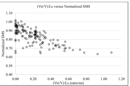
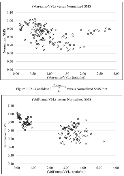
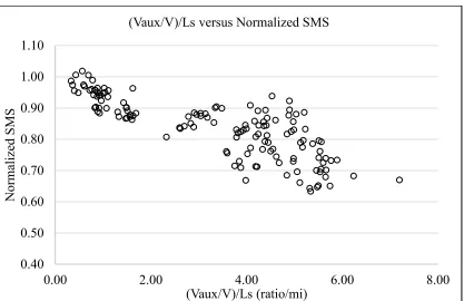
The candidate variables in SIW were tested based on the trend analyses that plotted each
variable against the normalized space mean speed. Figure 3.3 below illustrates the demand
variable plot that was used in this trend analysis. Figure 3.4 to Figure 3.24 below show the plots
of candidate variables in hypotheses 1, 2 and 3.
Figure 3.3 shows that has a relative strong trend with the normalized space mean speed
though the variance of the speed trendline increase with . It implies that the demand impacts
the segment average space mean speed, but there are also other potential factors influence the
speed drop which causes the observed variance. Figure 3.5 shows that most candidate 1 variables
do not have strong or moderate trend with speed changes except and . Figure 3.12
clearly indicates that the length of the segment is impacting the significance of the weaving
turbulence. The variables including , , , and , clearly shows a
relationship with speed changes. Interestingly, the variable plot shows that the speed drops
significantly when the ramp to ramp over segment length ratio is high. It signifies that the ramp
to ramp flow is influencing the segment average speed especially for the short segment. At last,
based on the observation of Figure 3.19,
( ), ( ), ( ), and ( ) are
proved that they have relationship with segment average speed changes. And again, the
( ) variable plot shows a very strong contribution to the speed drops.
Overall, the variables that have moderate to strong trends with space mean speed changes
are , , , , ,
non-correlated variables are then combined with each other to form multiple candidate model
forms that are shown in the next section.
Figure 3.3 - versus Normalized SMS Plot 0.40
0.50 0.60 0.70 0.80 0.90 1.00 1.10
0.00 0.20 0.40 0.60 0.80
N
or
m
al
iz
ed
S
M
S
(
O
bs
er
ve
d
sp
ee
d
/ F
FS
)
V/Cb
Figure 3.4 - Candidate 1 versus Normalized SMS Plot
Figure 3.5 - Candidate 1 versus Normalized SMS Plot 0.40
0.50 0.60 0.70 0.80 0.90 1.00 1.10
0.00 0.10 0.20 0.30 0.40 0.50 0.60 0.70
N
or
m
al
iz
ed
S
M
S
Vrf/V
Vrf/V versus Normalized SMS
0.40 0.50 0.60 0.70 0.80 0.90 1.00 1.10
0.00 0.10 0.20 0.30 0.40
N
or
m
al
iz
ed
S
M
S
Vfr/V
Figure 3.6 - Candidate 1 versus Normalized SMS Plot
Figure 3.7 - Candidate 1 VR versus Normalized SMS Plot 0.40
0.50 0.60 0.70 0.80 0.90 1.00 1.10
0.00 0.02 0.04 0.06 0.08
N
or
m
al
iz
ed
S
M
S
Vrr/V
Vrr/V versus Normalized SMS
0.40 0.50 0.60 0.70 0.80 0.90 1.00 1.10
0.00 0.20 0.40 0.60 0.80
N
or
m
al
iz
ed
S
M
S
VR
Figure 3.8 - Candidate 1 versus Normalized SMS Plot
Figure 3.9 - Candidate 1 versus Normalized SMS Plot 0.40
0.50 0.60 0.70 0.80 0.90 1.00 1.10
0.00 0.10 0.20 0.30 0.40 0.50 0.60 0.70
N
or
m
al
iz
ed
S
M
S
Von-ramp/V
Von-ramp/V versus Normalized SMS
0.40 0.50 0.60 0.70 0.80 0.90 1.00 1.10
0.00 0.10 0.20 0.30 0.40
N
or
m
al
iz
ed
S
M
S
Voff-ramp/V
Figure 3.10 - Candidate 1 versus Normalized SMS Plot 0.40
0.50 0.60 0.70 0.80 0.90 1.00 1.10
0.00 0.20 0.40 0.60 0.80
N
or
m
al
iz
ed
S
M
S
Vaux/V
Figure 3.11 - Candidate 2 versus Normalized SMS Plot
Figure 3.12 - Candidate 2 versus Normalized SMS Plot 0.40
0.50 0.60 0.70 0.80 0.90 1.00 1.10
0.00 0.50 1.00 1.50 2.00 2.50
N
or
m
al
iz
ed
S
M
S
Vrf/Ls (pc/hr/ft) Vrf/Ls versus Normalized SMS
0.40 0.50 0.60 0.70 0.80 0.90 1.00 1.10
0.00 1.00 2.00 3.00 4.00 5.00 6.00
T
it
le
Figure 3.13 - Candidate 2 versus Normalized SMS Plot
Figure 3.14 - Candidate 2 versus Normalized SMS Plot 0.40
0.50 0.60 0.70 0.80 0.90 1.00 1.10
0.00 0.20 0.40 0.60 0.80 1.00
N
or
m
al
iz
ed
S
M
S
Vrr/Ls (pc/hr/ft) Vrr/Ls versus Normalized SMS
0.40 0.50 0.60 0.70 0.80 0.90 1.00 1.10
0.00 1.00 2.00 3.00 4.00 5.00 6.00
N
or
m
al
iz
ed
S
M
S
Figure 3.15 - Candidate 2 versus Normalized SMS Plot
Figure 3.16 - Candidate 2 versus Normalized SMS Plot 0.40
0.50 0.60 0.70 0.80 0.90 1.00 1.10
0.00 0.50 1.00 1.50 2.00 2.50 3.00 3.50
N
or
m
al
iz
ed
S
M
S
Von-ramp/Ls (pc/hr/ft) Von-ramp/Ls versus Normalized SMS
0.40 0.50 0.60 0.70 0.80 0.90 1.00 1.10
0.00 1.00 2.00 3.00 4.00 5.00 6.00
N
or
m
al
iz
ed
S
M
S
Figure 3.17 - Candidate 2 versus Normalized SMS Plot 0.40
0.50 0.60 0.70 0.80 0.90 1.00 1.10
0.00 1.00 2.00 3.00 4.00 5.00 6.00 7.00
N
or
m
al
iz
ed
S
M
S
Vaxu/Ls
Figure 3.18 - Candidate 3 ( ) versus Normalized SMS Plot
Figure 3.19 - Candidate 3 ( ) versus Normalized SMS Plot 0.40
0.50 0.60 0.70 0.80 0.90 1.00 1.10
0.00 0.50 1.00 1.50 2.00 2.50 3.00
N
or
m
al
iz
ed
S
M
S
(Vrf/V)/Ls (ratio/mi) (Vrf/V)/Ls versus Normalized SMS
0.40 0.50 0.60 0.70 0.80 0.90 1.00 1.10
0.00 1.00 2.00 3.00 4.00 5.00 6.00
N
or
m
al
iz
ed
S
M
S
Figure 3.20 - Candidate 3 ( ) versus Normalized SMS Plot
Figure 3.21 - Candidate 3 versus Normalized SMS Plot 0.40
0.50 0.60 0.70 0.80 0.90 1.00 1.10
0.00 0.20 0.40 0.60 0.80 1.00 1.20
N
or
m
al
iz
ed
S
M
S
(Vrr/V)/Ls (ratio/mi) (Vrr/V)/Ls versus Normalized SMS
0.40 0.50 0.60 0.70 0.80 0.90 1.00 1.10
0.00 2.00 4.00 6.00 8.00
N
or
m
al
iz
ed
S
M
S
Figure 3.22 - Candidate 3 ( ) versus Normalized SMS Plot
Figure 3.23 - Candidate 3 ( ) versus Normalized SMS Plot 0.40
0.50 0.60 0.70 0.80 0.90 1.00 1.10
0.00 0.50 1.00 1.50 2.00 2.50 3.00
N
or
m
al
iz
ed
S
M
S
(Von-ramp/V)/Ls (ratio/mi) (Von-ramp/V)/Ls versus Normalized SMS
0.40 0.50 0.60 0.70 0.80 0.90 1.00 1.10
0.00 1.00 2.00 3.00 4.00 5.00 6.00
N
or
m
al
iz
ed
S
M
S
Figure 3.24 - Candidate 3 ( ) versus Normalized SMS Plot 0.40
0.50 0.60 0.70 0.80 0.90 1.00 1.10
0.00 2.00 4.00 6.00 8.00
N
or
m
al
iz
ed
S
M
S
CHAPTER 4 : MODEL RESULTS 4.1 Candidate Model Forms and Model Calibration:
Twelve candidate model forms were created during the calibration, as listed below. It
should be noted that Model 5 contained a variable that has not been explained. The term
∗
is a transformation from the volume ratio. Because several prior works have shown
that on-ramp traffic has more contribution to the speed drop, it adds a weighting factor ‘a’ for the
ramp to freeway volume. Model forms 6 to 10 were motivated by the calibration results from
Model 1 to Model 4, because either had a negative parameter that is counterintuitive or proved
to be insignificant. Model 11 and 12 were the transformation from Model 8 and Model 9 which
separate the segment length as an independent variable.
Interestingly, these model forms can conceptually fit the ramp junctions as well. For
example, when Model 1 is used to predict the speed of a merging section, the variable will
become zero and the variable will present the ratio of merging demand over acceleration lane
length. But further studies are needed to validate this conceptual approach, this paper is focusing
on ramp weaves only.
Model 1: 𝑆 = 𝑆 − 𝛼 ∗ 𝐹𝐹𝑆 ∗ ∗ ∗
Model 2: 𝑆 = 𝑆 − 𝛼 ∗ 𝐹𝐹𝑆 ∗ ∗ ∗
Model 3: 𝑆 = 𝑆 − 𝛼 ∗ 𝐹𝐹𝑆 ∗ ∗
( )
Model 4: 𝑆 = 𝑆 − 𝛼 ∗ 𝐹𝐹𝑆 ∗ ∗
Model 5: 𝑆 = 𝑆 − 𝛼 ∗ 𝐹𝐹𝑆 ∗ ∗ ∗
( )
Model 6: 𝑆 = 𝑆 − 𝛼 ∗ 𝐹𝐹𝑆 ∗ ∗
Model 7: 𝑆 = 𝑆 − 𝛼 ∗ 𝐹𝐹𝑆 ∗ ∗
Model 8: 𝑆 = 𝑆 − 𝛼 ∗ 𝐹𝐹𝑆 ∗
( ) ∗ ( )
Model 9: 𝑆 = 𝑆 − 𝛼 ∗ 𝐹𝐹𝑆 ∗
( ) ∗ ( )
Model 10: 𝑆 = 𝑆 − 𝛼 ∗ 𝐹𝐹𝑆 ∗ ∗
( )
Model 11: 𝑆 = 𝑆 − 𝛼 ∗ 𝐹𝐹𝑆 ∗ ∗ ∗ 𝐿 (𝑖𝑛 𝑚𝑖𝑙𝑒𝑠)
Model 12: 𝑆 = 𝑆 − 𝛼 ∗ 𝐹𝐹𝑆 ∗ ∗ ∗ 𝐿 (𝑖𝑛 𝑚𝑖𝑙𝑒𝑠)
All the model forms above were then transformed into linearized forms, was shown in
Equation (9). The parameters were calibrated using linear regression. However, due to the fact
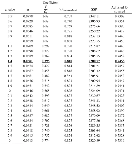
that the Model 5 was still non-linear after transformation, a different approach was applied to it.
The ‘a’ value was tested within a range of values from 0.5 to 3.0. The linear regression analysis
was applied for each ‘a’ value assigned model. The optimal ‘a’ value was determined by
comparing the best goodness of fit among the models. The detailed model calibration result for
different ‘a’ value assigned to Model 5 is shown in Table 4.1. It should be noted that for the ‘a’
value from 0.5 to 1, the was not significant in the model, so there is no coefficient that can be
the best adjusted R-squared value and the lowest sum of squared residual. Table 4.2 below shows
the parameter calibration result for all candidate models
Table 4.1
Parameter Calibration Result and Goodness of Fit for Different ‘a’ Value Models
Coefficient
a value α V
𝐶 VR SSR
Adjusted R-squared
0.5 0.0778 NA 0.707 2347.11 0.7308
0.6 0.0729 NA 0.740 2306.93 0.7354
0.7 0.0685 NA 0.769 2275.66 0.7390
0.8 0.0646 NA 0.795 2250.22 0.7419
0.9 0.0611 NA 0.818 2232.13 0.7440
1 0.0579 NA 0.838 2223.55 0.7450
1.1 0.0709 0.292 0.790 2215.87 0.7440
1.2 0.0698 0.327 0.798 2208.62 0.7448
1.3 0.0689 0.362 0.804 2205.55 0.7452
1.4 0.0681 0.395 0.810 2200.77 0.7458
1.5 0.0674 0.427 0.814 2201.21 0.7457
1.6 0.0667 0.458 0.818 2203.32 0.7455
1.7 0.0661 0.487 0.82 1 2205.91 0.7452
1.8 0.0656 0.515 0.823 2209.94 0.7447
1.9 0.0651 0.542 0.825 2214.89 0.7441
2 0.0646 0.568 0.826 2224.09 0.7431
2.1 0.0642 0.593 0.827 2230.67 0.7423
2.2 0.0638 0.617 0.827 2241.33 0.7411
2.3 0.0634 0.640 0.828 2248.52 0.7402
2.4 0.0631 0.661 0.827 2258.92 0.7390
2.5 0.0627 0.682 0.827 2270.09 0.7377
2.6 0.0624 0.702 0.827 2277.80 0.7368
2.7 0.0621 0.721 0.826 2289.25 0.7355
2.8 0.0618 0.740 0.825 2301.64 0.7341
2.9 0.0615 0.757 0.824 2312.62 0.7328
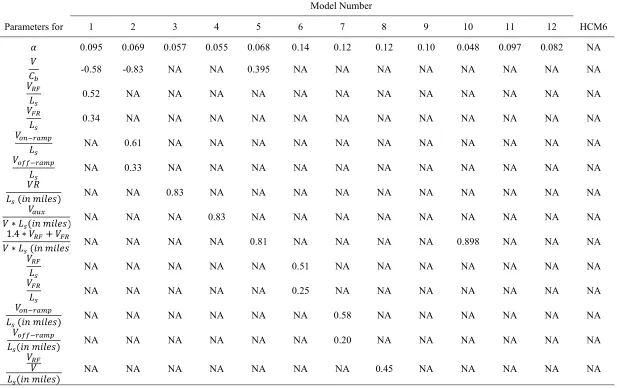
Table 4.2
Model Calibration Results and Goodness of Fit Comparison Between Candidate Models and HCM6
Model Number
Parameters for 1 2 3 4 5 6 7 8 9 10 11 12 HCM6
𝛼 0.095 0.069 0.057 0.055 0.068 0.14 0.12 0.12 0.10 0.048 0.097 0.082 NA
𝑉
𝐶 -0.58 -0.83 NA NA 0.395 NA NA NA NA NA NA NA NA
𝑉
𝐿 0.52 NA NA NA NA NA NA NA NA NA NA NA NA
𝑉
𝐿 0.34 NA NA NA NA NA NA NA NA NA NA NA NA
𝑉
𝐿 NA 0.61 NA NA NA NA NA NA NA NA NA NA NA
𝑉
𝐿 NA 0.33 NA NA NA NA NA NA NA NA NA NA NA
𝑉𝑅
𝐿 (𝑖𝑛 𝑚𝑖𝑙𝑒𝑠) NA NA 0.83 NA NA NA NA NA NA NA NA NA NA 𝑉
𝑉 ∗ 𝐿 (𝑖𝑛 𝑚𝑖𝑙𝑒𝑠) NA NA NA 0.83 NA NA NA NA NA NA NA NA NA 1.4 ∗ 𝑉 + 𝑉
𝑉 ∗ 𝐿 (𝑖𝑛 𝑚𝑖𝑙𝑒𝑠) NA NA NA NA 0.81 NA NA NA NA 0.898 NA NA NA 𝑉
𝐿 NA NA NA NA NA 0.51 NA NA NA NA NA NA NA
𝑉
𝐿 NA NA NA NA NA 0.25 NA NA NA NA NA NA NA
𝑉
𝐿 (𝑖𝑛 𝑚𝑖𝑙𝑒𝑠) NA NA NA NA NA NA 0.58 NA NA NA NA NA NA 𝑉
𝐿 (𝑖𝑛 𝑚𝑖𝑙𝑒𝑠) NA NA NA NA NA NA 0.20 NA NA NA NA NA NA 𝑉
𝑉
Table 4.2
Model Calibration Results and Goodness of Fit Comparison Between Candidate Models and HCM6 (Continued)
Model Number
Parameters for 1 2 3 4 5 6 7 8 9 10 11 12 HCM6
𝑉 𝑉
𝐿 (𝑖𝑛 𝑚𝑖𝑙𝑒𝑠) NA NA NA NA NA NA NA 0.40 NA NA NA NA NA 𝑉
𝑉 𝐿 (𝑖𝑛 𝑚𝑖𝑙𝑒𝑠)
NA NA NA NA NA NA NA NA 0.51 NA NA NA NA
𝑉 𝑉 𝐿 (𝑖𝑛 𝑚𝑖𝑙𝑒𝑠)
NA NA NA NA NA NA NA NA 0.37 NA NA NA NA
𝑉
𝑉 NA NA NA NA NA NA NA NA NA NA 0.45 NA NA
𝑉
𝑉 NA NA NA NA NA NA NA NA NA NA 0.35 NA NA
𝑉
𝑉 NA NA NA NA NA NA NA NA NA NA NA 0.51 NA
𝑉
𝑉 NA NA NA NA NA NA NA NA NA NA NA 0.30 NA
𝐿 NA NA NA NA NA NA NA NA NA NA -0.91 -0.94 NA
SSR 2242 1835 2224 2064 2201 2359 2126 1923 1663 2241 1893 1637 8727
SST 8847 8847 8847 8847 8847 8847 8847 8847 8847 8847 8847 8847 8847
Adjusted
R-squared 0.747 0.793 0.749 0.767 0.751 0.733 0.760 0.783 0.812 0.743 0.780 0.809 0.013
AICc 794.91 765.86 788.52 778.07 789.17 798.88 784.32 770.28 749.98 789.59 770.18 749.88 977.89
By applying the results of the analysis to the model formula, the final models with
significant variables and calibrated parameters are listed below:
Model 1: 𝑆 = 𝑆 − 0.0952 ∗ 𝐹𝐹𝑆 ∗ . ∗ . ∗ .
Model 2: 𝑆 = 𝑆 − 0.0699 ∗ 𝐹𝐹𝑆 ∗ . ∗ . ∗ .
Model 3: 𝑆 = 𝑆 − 0.0579 ∗ 𝐹𝐹𝑆 ∗
( ) .
Model 4: 𝑆 = 𝑆 − 0.0555 ∗ 𝐹𝐹𝑆 ∗
∗ ( ) .
Model 5: 𝑆 = 𝑆 − 0.0681 ∗ 𝐹𝐹𝑆 ∗ . ∗ . ∗
∗ ( ) .
Model 6: 𝑆 = 𝑆 − 0.140 ∗ 𝐹𝐹𝑆 ∗ . ∗ .
Model 7: 𝑆 = 𝑆 − 0.124 ∗ 𝐹𝐹𝑆 ∗
( ) .
∗
( )
.
Model 8: 𝑆 = 𝑆 − 0.125 ∗ 𝐹𝐹𝑆 ∗
( )
. ∗
( )
.
Model 9: 𝑆 = 𝑆 − 0.109 ∗ 𝐹𝐹𝑆 ∗
( )
. ∗
( )
.
Model 10: 𝑆 = 𝑆 − 0.0481 ∗ 𝐹𝐹𝑆 ∗ . ∗
∗ ( ) .
Model 11: 𝑆 = 𝑆 − 0.0975 ∗ 𝐹𝐹𝑆 ∗ . ∗ . ∗ (𝐿 (𝑚𝑖𝑙𝑒𝑠)) .
Model 12: 𝑆 = 𝑆 − 0.0824 ∗ 𝐹𝐹𝑆 ∗ . ∗ . ∗ (𝐿 (𝑚𝑖𝑙𝑒𝑠)) .