Scholarship at UWindsor
Scholarship at UWindsor
Electronic Theses and Dissertations Theses, Dissertations, and Major Papers
2013
Comparative Study of Sampling Methods for Online Social
Comparative Study of Sampling Methods for Online Social
Networks
Networks
Hao Wang
University of Windsor
Follow this and additional works at: https://scholar.uwindsor.ca/etd
Recommended Citation Recommended Citation
Wang, Hao, "Comparative Study of Sampling Methods for Online Social Networks" (2013). Electronic Theses and Dissertations. 4871.
https://scholar.uwindsor.ca/etd/4871
This online database contains the full-text of PhD dissertations and Masters’ theses of University of Windsor students from 1954 forward. These documents are made available for personal study and research purposes only, in accordance with the Canadian Copyright Act and the Creative Commons license—CC BY-NC-ND (Attribution, Non-Commercial, No Derivative Works). Under this license, works must always be attributed to the copyright holder (original author), cannot be used for any commercial purposes, and may not be altered. Any other use would require the permission of the copyright holder. Students may inquire about withdrawing their dissertation and/or thesis from this database. For additional inquiries, please contact the repository administrator via email
Comparative Study of Sampling
Methods for Online Social Networks
by
Hao Wang
A Thesis
Submitted to the Faculty of Graduate Studies
through Computer Science
in partial fulfilment of the requirements for
the Degree of Master of Science at the
University of Windsor
Windsor, Ontario, Canada
2013
c
by
Hao Wang
APPROVED BY:
Dr. Zhiguo Hu, External Reader Department of Mathematics and Statistics
Dr. Luis Rueda, Internal Reader School of Computer Science
Dr. Jianguo Lu, Advisor School of Computer Science
Dr. Arunita Jaekel, Chair of Defense School of Computer Science
Declaration of
Co-Authorship/Previous
Publication
1. Declaration of Co-Authorship
I hereby declare that this thesis incorporates the outcome of joint research undertaken
under the supervision of Dr. Jianguo Lu. The collaboration is covered in Chapters 2,
3, 4 and 5 of the thesis. In all cases, I conducted all the experiments including data
collection and analysis.
I certify that I have properly acknowledged the contribution of other researchers to my
thesis, and have obtained written permission from the co-author to include the above
material(s) in my thesis.
I certify that, with the above qualification, this thesis, and the research to which it
refers, is the product of my own work.
2. Declaration of Previous Publication
This thesis includes four original papers that have been previously submitted to the
journal and conference, as follows:
I certify that I have obtained written permission from the copyright owner(s) to
in-clude the above published material(s) in my thesis. I certify that the above material
describes work completed during my registration as graduate student at the University
of Windsor.
I declare that, to the best of my knowledge, my thesis does not infringe upon anyone‘s
copyright nor violate any proprietary rights and that any ideas, techniques, quotations,
or any other material from the work of other people included in my thesis are fully
acknowledged. Furthermore, to the extent that I have included copyrighted material
that surpasses the bounds of fair dealing within the meaning of the Canada Copyright
2 Hao Wang, Jianguo Lu, Uniform Random Sampling on Graph: To Be or Not To Be?
Submitted to Information Process-ing and Management(IPM), 2013.
3 Hao Wang, Jianguo Lu,
Uni-form Random Sampling not Recom-mended for Size Estimation.
Submitted to Physica A: Statisti-cal Mechanics and its Applications, 2013.
4 Hao Wang, Jianguo Lu, Detect
In-flated Follower Numbers in OSN Us-ing Star SamplUs-ing.
Submitted to The 2013 IEEE/ACM International Conference on Ad-vances in Social Networks Analysis and Mining, 2013.
5 Hao Wang, Jianguo Lu, What Do
Large Networks Look Like?
Submitted to The 19th ACM
SIGKDD Conference on Knowledge, Discovery, and Data Mining, Work-shop, 2013.
Act, I certify that I have obtained a written permission from the copyright owner(s)
to include such material(s) in my thesis.
I declare that this is a true copy of my thesis, including any final revisions, as approved
by my thesis committee and the Graduate Studies office, and that this thesis has not
Abstract
The properties of online social networks are of great interests to the general public as well
as IT professionals. Often the raw data are not available and the summaries released by
the service providers are sketchy. Thus sampling is needed to reveal the hidden
proper-ties and structure of the underlying network. This thesis conducts comparative studies on
various sampling methods, including Random Node(RN), Random Walk(RW) and Random
Edge(RE) samplings. The properties to be discovered include the average degree and
popu-lation size of the network. Additionally, this thesis proposes a new sampling method called
STAR sampling and applies this method to an online social network Weibo. Furthermore,
visualization of network structure is studied to explain the impact of network structure on the
performance of sampling methods. We show that RE sampling is better than RN sampling
in general. This result is supported by over 20 real-world networks.
To my grandmother Suzhen Zhang(1927 - 2013)
for teaching me to be a honest and hard-work person.
Acknowledgements
I would like to acknowledge the important role of my thesis committee members and thank
them for their enlightening and encouraging comments and reviews.
I wish to express my great gratitude to my supervisor Dr.Jianguo Lu for his valuable assistance
and support during my thesis work, and for his persistent guidance throughout my study
during master program.
My parents’ unconditional love guide me through my life and I am grateful to my parents for
providing me with flesh and soul. A heartfelt thanks goes out to my girlfriend Shuangshuang
Dong for all your love, support and patience while we are seperated distantly.
To all who help me get through the graduate time.
Declaration of Co-Authorship/Previous Publication iii
Abstract v
Dedication vi
Acknowledgements vii
List of Figures ix
List of Tables x
1 Introduction 1
1.1 Motivation . . . 1
1.2 Average Degree Estimation . . . 2
1.3 Size Estimation . . . 3
1.4 Follower Estimation . . . 4
1.5 Visualization . . . 5
2 Uniform Random Sampling on Graph: To Be or Not To Be? 6 2.1 Introduction. . . 7
2.2 Related work . . . 9
2.3 Sampling methods and their estimators . . . 11
2.3.1 The problem . . . 11
2.3.2 RN sampling . . . 12
2.3.3 RE and RW Sampling . . . 13
2.3.4 Other estimators . . . 14
2.4 Experiments. . . 15
2.4.1 Datasets. . . 15
2.4.2 RE vs. RN sampling . . . 17
2.4.3 RW vs. RN sampling . . . 20
2.5 Conclusions . . . 22
2.6 Acknowledgements . . . 24
2.7 Appendix . . . 25
2.7.1 Proof of Theorem 1 . . . 25
2.7.2 Proof of Theorem 2 . . . 25
3 Uniform Random Sampling not Recommended for Size Estimation 27 3.1 Introduction. . . 28
3.2 Background and Related Work . . . 29
3.2.1 Random Node Sampling . . . 29
3.2.2 Sampling Nodes With Unequal Probability . . . 30
3.2.3 Evaluation of Estimation Methods . . . 32
3.2.4 Graph Sampling . . . 32
3.2.5 Other Size Estimation Approaches . . . 33
3.3 Random Node (RN) Sampling. . . 33
3.4 Random Edge (RE) Sampling . . . 36
3.5 Random Walk (RW) Sampling . . . 39
3.6 Discussions and Conclusions . . . 41
3.7 Appendix . . . 42
3.7.1 Proof of Lemma 1 . . . 42
3.7.2 Proof of Lemma 2 . . . 43
4 Detect Inflated Follower Numbers in OSN Using Star Sampling 45 4.1 introduction . . . 46
4.2 Background and Related Work . . . 47
4.2.1 OSN Access Methods . . . 47
4.2.2 Graph sampling . . . 48
4.2.2.1 Uniform Random Node Sampling . . . 48
4.2.2.2 Random edge sampling . . . 48
4.2.2.3 Random walk sampling . . . 48
4.2.3 Weibo and other OSN sampling. . . 49
4.3 Uniform ID Sampling and Size Estimation . . . 49
4.3.1 Degree and message distributions . . . 50
4.4 Star sampling and Follower Number Estimation . . . 52
4.4.1 Star sampling . . . 53
4.4.2 Pilot study on local datasets . . . 55
4.4.3 Results for Weibo data. . . 57
4.5 Discussions and Conclusions . . . 59
4.6 Acknowledgement. . . 60
4.7 Appendix . . . 60
5 What Do Large Networks Look Like? 61 5.1 Introduction. . . 62
5.2 Our method . . . 63
5.3 Community structure . . . 64
5.4 Conclusions . . . 68
Bibliography 69
Bibliography 75
2.1 A graph and three sampling methods to select six sample nodes. The three sampling methods are random node (RN), random edge (RE), and random walk (RW). Nodes can be sampled multiple times as shown in sub-figures for RE and RW samplings. . . 7
2.2 Degree distributions of 18 graphs. Plots are sorted in decreasing order of coefficient of variation γ. Graphs in the last row have small γ values because the maximal degree is small compared to the data size. For these graphs RE sampling does not have obvious advantage. Web graphs (sub-figures 3, 5, 8) do not form a straight line in the upper part of the log-log plots, indicating irregularity in the graph structure. For these graphs simple RW sampling should be avoided. . . 17
2.3 Summary of the three sampling methods on 18 graphs. (A) Comparison in terms of RRMSEs. (B) The advantage of RE grows as a linear function of γ. It shows that RRMSE of RN/RE grows almost linearly with γ. Pearson’s coefficient of correlation is 0.9354. Inset: there are four cases where RN/RE is smaller than one. These four graphs from left to right are RoadNet, Citation, Facebook-2, and Flickr. In both (A) and (B) the sample size is 400, and RRMSEs are obtained over 5000 runs except for Twitter data that has 2000 runs. . . 18
2.4 RRMSEs of RN, RE, and RW samplings as a function of sample size for 18 graphs. The dotted, dashed, and solid lines are for RN(. . .), RE(−−), and RW(–) samplings respectively. It shows that in most cases the sample size does not change the relative positions of the sampling methods. The exceptions are the web graphs 3 and 5 where RW sampling does not improve with the increase of sample size because of the random walk traps. 19
2.5 The degree distributions of the samples obtained from RE (Random Edge) samplings. n=8,000. The log-log plots in the first two rows exhibit a “V” shape, where the sampled small nodes resemble the distribution of the original graph, while the sampled large nodes have a tail pointing upwards. These plots in the first two rows indicate that both small and large nodes are well represented in the sample. The plots in the last row indicate that the sample distribution is similar to the original distribution, therefore the RRMSE of RE sampling is similar to that of RN sampling. . 19
2.6 Standard error ratio between RW and RE vs. graph conductance Φ for 18 datasets. Sample size is 400. . . 22
2.7 (Best viewed in colour) Random walks on six networks. Flickr, NotreDame and Stanford have loosely connected components while Amazon, Face-book and Youtube are well enmeshed. Each random walk contains 6×10⁴ nodes except NotreDame which has 15×104 nodes. Node colour indicates the degree of the node. Green=1; Blue=2∼9; Yellow=10∼99; Red=100+. 23
2.8 Conductance Φ(S) over |S|, the size of the the components, for six net-works. Plots are drawn using SNAP API described in [1]. . . 23
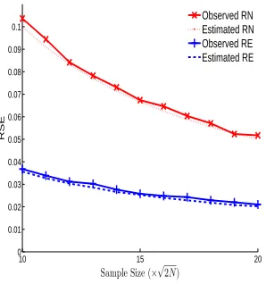
3.1 Relative standard errors of RE and RN samplings on Facebook data when sample size ranges between 10×√2N and 20×√2N, where√2N = 2423. The red lines are for RN sampling and blue lines are for RE sampling. . 35
3.2 Comparison of RE and RN in terms of standard error when the sample size of RE is √Γ times smaller than that of RN, for 18 datasets. The expectedC for both RE and RN sampling is 100. . . 35
3.3 Estimated and observed RSE of RE sampling with the growth of sample size over 18 datasets. The sample size ranges between 10×p
2N/Γ and 20×p2N/Γ, i.e., the expected collisions are between 100 and 400. . . . 36
3.4 Comparison of three sampling methods. The sample size n = √2N C
where √C = 10. It shows that for RN sampling (red solid bars), the relative standard error is equal to 1/√C = 0.1 across all the datasets. RE sampling is consistently smaller than RN sampling, and decreases with the growth of γ. RW sampling can approximate RE sampling for some datasets. For NotreDame etc. that have low conductance, RW is grossly wrong. . . 37
3.5 (Better viewed in colour) Subgraphs obtained by RW sampling from Flickr, EmailEu, Stanford and Youtube. Each subgraph contains 60,000 nodes. Node colour represents its degree in the original graph. Green=1; Blue=2 ∼9; Orange= 10∼99; Red=100∼ ∞. . . 38
3.6 The ratio of RSEs between RW and RE samplings over the conductance Φ. For the four graphs with the lowest conductance, RW is around 10 times worse than RE sampling. Sample sizen=p2N E(C) whereE(C) = 100. RSE is obtained over 3000 runs.. . . 40
4.1 Estimated number of accounts against sample size. The estimation sta-bilizes when only 20,000 random IDs are tested.. . . 51
4.2 Estimated out-degree, in-degree, and message distributions of Weibo. . . . 52
4.3 Degree estimation of six networks using star sampling. Boxplots are ob-tained from 100 repeated experiments. . . 56
4.4 Weibo followers estimation. Panel A: inflation ration over 104 top ac-counts. Panel B: the smoothed version of A. Panel C: All the accounts whose inflation ratio is higher than one. Panel D: top 500 accounts. Panel E: comparison of top 104accounts, smoothed. Panel F: difference between the claimed and estimated followers. Smoothed.. . . 58
4.5 Estimated followers vs. claimed followers. The Pearson correlation coef-ficient is 0.9797.. . . 59
5.1 Visualization of Twitter user network. . . 66
5.2 Conductance Φ(S) over |S|, the size of the the components, for six net-works. Insets: The corresponding NCP plots obtained from the subgraphs. 67
2.1 Summary of notations . . . 11
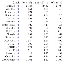
2.2 Statistics of the 18 graphs, sorted in decreasing order of the coefficient of degree variation γ. Each graph has a citation indicating where the data is from. . . 15
3.1 Statistics of the 18 real-world graphs, sorted in descending order of the coefficient of degree variation γ. Φ is the conductance. . . 34
4.1 Statistics of the 6 real-world graphs, sorted in descending order of the coefficient of degree variation γ =variance/hdi2. . . . 57
4.2 Estimation for the top 10 Weibo accounts. fi: capture frequency of the
account i; di claimed in-degree or number of followers; hcdii: estimated number of followers. . . 57
5.1 Statistics of the six networks, each has a citation indicating where the data is from. hdiis the average degree, CV stands for coefficient of variation. 65
Introduction
1.1
Motivation
The properties and structure of online social networks are of interest to a variety of
stakeholders, including the general public as well as IT professionals. With the
knowl-edge of the topology of the network, users can post their status on the network, so that
their information can diffuse more effectively. Often the raw data are not available and
the summaries released by the service providers are sketchy. Thus sampling is needed
to reveal the hidden structure of the underlying data.
Online social networks are so large that exhaustive exploration of the network is
in-feasible. In fact, we can only obtain a small sample of the network and estimate the
properties of the network using the sample.
For instance, we may want to learn the average number of followers in the network,
or the average in degree of the graph. One obvious but often impractical method is to
select randomly a set of users{U1, U2. . . , Un}, count the in-degrees{d1, . . . , dn}for each
user, and calculate the sample mean d
d= 1
n
n
X
i=1
di (1.1)
The sample mean is an unbiased estimator of the population if the users can be selected
randomly with uniform distribution. Unfortunately this is not the case in practice.
When microbloggers are selected, they are often not picked randomly due to the limited
access methods.
Average degree is just one of the many properties that are of interest. Other properties
include the order (the number of nodes), the size (the number of edges) of the graph, the
distribution of degrees, the diameter of the graph, the centralities commonly used in
so-cial network measurement such as betweenness, the closeness, the eigenvector centrality,
the clustering coefficients. All those properties can be calculated with the presence of
the complete data, even though some of the properties can not be computed efficiently.
Different sampling methods shall be employed depending on the properties we want to
reveal. On the one hand, we need to learn the macroscopic properties such as size of the
network and the average number of followers. These properties can be better discovered
using uniform sampling, i.e., every account is sampled using equal probability. On the
other hand, it is interesting to find out the top bloggers, their topological structure,
or even clusters. Those top bloggers are easier to have higher probabilities of being
sampled.
This thesis contains four papers addressing different aspects of OSNs analysis including
degree estimation, size estimation, follower estimation and visualization. The following
sections in this chapter introduce the background in general terms of four papers.
1.2
Average Degree Estimation
The norm of practice in estimating graph properties is to obtain uniform random (node)
samples whenever possible. Often uniform random node (RN) samples are hard to
obtain, henceforth the less costly simple random walk (RW) sampling is applied instead.
Chapter 2 contains our paper that tries to answer the question as for which method
is better in estimating average degree, disregarding the extra cost to obtain uniform
random samples by methods such as rejection sampling. Two basic sampling schemas
are UR(Uniform Random) sampling and PPS(Probability Proportional to Size)
sam-pling. In UR sampling, each node is sampled with equal probability, thus the sample
(dx1, dx2, . . . , dxn) is uniform at random. The arithmetic mean is applied in estimating
average degree:
c
hdiU R = 1
n
n
X
i=1
In PPS sampling a node is sampled with probability proportional to its size. The
harmonic mean is used:
c
hdiP P S =n
" n X
i=1 1
dxi
#−1
Corresponding to these two basic sampling schemes, a graph can be sampled by RN(Random
Node) and RE/RW(Random Edge/Random Walk) sampling methods. We conduct
ex-periments on 18 real-worlk large networks and evaluate the accuracy of three sampling
methods in terms of RRMSE(Relative Rooted Mean Square Error).
After comparing the results of the sampling methods, we find that when the network
is large and scale-free, RE sampling is much better than RN sampling and even if the
network is not large or not following the right distribution, we still can distinguish the
good from the bad by using the coefficient of variation of the degree.
Since RE is not practical in some real applications, we use RW sampling instead. From
the comparison, we also find that RW can be better than the costly RN in orders of
magnitude for some datasets, yet it can be worse for some other datasets, depending
on the degree variance and conductance of the graph. Furthermore, we show the ratio
between RW and RE sampling depends on the structure of the graph which we use
conductance to describe.
1.3
Size Estimation
Chapter 3 contains our paper that describes the performance of different sampling
methods in estimating the network population. Population is the very fundamental
property of the network and size estimation has been widely studied. As same as average
degree estimation, we still compare RN, RW and RE sampling methods. The estimator
for RN sampling is:
b
NN =
n
2
1
C ≈ n2
2C.
While the estimator for RW and RE sampling is:
b
NE = Γ
n
2
1
C ≈bΓ n2
2C
Based on these two estimators, we derive the variance for RN sampling and RE sampling.
We verify the estimated variance with the observed variance from the experiment and
they agree with each other very well. This gives us the confidence to further quantify
the difference between RE and RN sampling methods. The only difference between
RE and RN sampling is Γ and this suggests that with the same sample size n, RE
sampling creates Γ times more collisions. Therefore the variance of NbE is smaller by a
factor of Γ. The experiment result confirms that√Γ is the upper bound for the ratio of
RSEs(Relative Standard Error) between RE and RN sampling methods.
We also use RW sampling to approximate RE sampling since RE is rarely possible in
real applications. We find that random walk mixing time plays an important role in the
performance of size estimation. If there is no loosely connected components existing,
RW is better than RN, otherwise, RW will be increadibly bad.
1.4
Follower Estimation
Chapter 4 contains our paper which describes follower estimation by a high-efficient
sampling method called STAR sampling and this sampling method derived from simple
RW sampling. Different from simple RW sampling that takes only one sample at each
step, STAR sampling takes all the neighbours as valid samples. As a result, It is more
efficient than random walk sampling by a factor of the average degree. Moreover, STAR
sampling is a kind of PPS sampling indicating large nodes will be sampled with higher
frequency which are proportional to their degrees. We benifit from this character that
we can easily focus on the sub graphs of the top users.
We apply STAR sampling in estimating the number of followers of the top nodes who
have the most links in the graph. We first conduct experiment on six local datasets
whose ground-truth are known. The results on six networks show that our method
works very well as the empirical results according to the true values.
Then we apply our method on Weibo, the Chinese version of Twitter, whose properties
are rarely studied albeit its enormous size and inuence. Before applying star sampling,
we use ID sampling(known as Rejection-Acceptance Sampling) to estimate the size of
Weibo. The sample obtained by ID sampling is a uniform random sample, as the
by-product of the uniform random sample, the degree distribution has been plotted to give
a direct impression of Weibo. Surprisingly, we find that the average in-degree is larger
than the average out-degree.
We explain this by investigating the number of followers for the users in the network.
of followers of the top 1000 users. In general the estimated follower number is consistent
with the claimed number, but there are cases that the follower numbers are inflated by
a factor up to 132.
1.5
Visualization
Chapter 4contains our paper that uses random spanning tree to visualize large online
social networks. Since visulization could bring too much benifit to realize the topology
of large networks, many research works have been done to draw the structure of large
graphs. However, most approaches can only handle small graphs with a couple hundred
nodes and edges. To show the overall structure of OSNs with huge size, we reduce the
number of nodes and edges by producing a representative subgraph. This subgraph is
produced by simple random walk, due to its PPS character, the nodes are sampled with
probability proportional to their degrees, so that large nodes with more connections have
a higher probability of being sampled. The edges are reduced further using uniform
random spanning tree. We use NCP(Network Community Profile) plots to explain
that the subgraph produced by our method preserves the structure of original graph,
thus it is representative. Lastly, we visualize six real-world networks and explain their
Uniform Random Sampling on
Graph: To Be or Not To Be?
This paper was submitted as:
Hao Wang, Jianguo Lu, Uniform Random Sampling on Graph: To Be or Not To Be?.
Information Processing and Management(IPM), 2013, submitted.
2 2
1 6
3
3 5
3 1
4
1 1
2
1 3
5 3
4
Original graph Random Node
6 3
3 5
3
2
6 3
3 5
Random Edge Random Walk
Figure 2.1: A graph and three sampling methods to select six sample nodes. The
three sampling methods are random node (RN), random edge (RE), and random walk (RW). Nodes can be sampled multiple times as shown in sub-figures for RE and RW
samplings.
2.1
Introduction
Many datasets can be viewed as graphs, especially the Web and online social networks
such as Twitter and Facebook. These graphs are large, and sometimes are hidden behind
searchable interfaces. Thus, the direct process of the graphs is not efficient or feasible,
and sampling is the other option to reveal the hidden properties or structure of the
underlying data. In the past, extensive research was carried out to explore the profile of
search engines [2] and other data collections [3–5]. Many of them focused on obtaining
uniform random samples [6,7]. Recently the problem becomes more urgent due to the
wide spread adoption of big data, resulting in a spate of research on this topic, such as
[8–13] to name a few of them.
Two of the basic sampling methods are uniform random sampling and PPS
(Probability-Proportional-to-Size) sampling. In uniform random sampling, each item is sampled with
equal probability. In PPS sampling an item is sampled with probability proportional to
its size. Corresponding to these two basic sampling schemes a graph can be sampled by
random nodes (RN) and random edges (RE) as illustrated in Figure2.1. In random node
sampling, each node is sampled uniform randomly. In random edge sampling, two nodes
incident to a random edge are collected. Random walk (RW) sampling approximates the
A fundamental question in graph sampling is which sampling method is better. There
is no single answer to this question because it depends on the graph properties to be
revealed, and the graph structure being investigated [10]. This paper tries to answer a
narrowed-down question: which sampling method is better for estimating the average
degree of a scale-free graph? By focusing on one property, we can give a more definite
answer, and then expand the answer to other properties. Average degree itself is an
important metric for any network. Furthermore, it can lead to the discovery of other
properties such as the population size of a network [14,15], the variation of the degrees,
and even the threshold value for the occurrence of large components in message diffusion
[16]. Section 2.3.4will discuss the utilization of the average degree in the estimation of
these properties in more details.
While it is easy to understand that RN sampling does not work well for scale-free
networks due to its large variation of degrees, it is far from clear whether other sampling
methods can reduce the variance. Take Twitter and Facebook, two popular online
social networks, for example. They are both scale-free networks, yet they favour different
sampling methods. Twitter prefers RE sampling, but Facebook is the other way around.
What is more surprising is that for Twitter network, RE sampling is hundreds of times
better than RN sampling in terms of sample size. Such huge difference has a great
impact on the theory and practice of big data analysis. In practice, the selection of
the correct sampling method can save the cost in orders of magnitude. In theory, new
sampling methods need to be developed to exploit this difference. Naturally, we ponder
when RE is better than RN sampling, and how much better it can be in reality.
The main contribution of this paper is that the normalized variance of the degrees
dictates the sampling method we should use. More precisely, the ratio of the estimation
errors between RE and RN samplings can be quantified by the coefficient of variation
(γ) of the degrees of the data. Their Pearson’s correlation coefficient is as high as 0.9354 among 18 networks we studied. In theory, the variance and γ may not exist when the slope of the power law distribution is between 1 and 2. In practice, all the real networks
have a maximal degree, resulting in a bounded variance for each network. Among 18
networks we studied, most of them have γ ranging between 1 and 36. In other words, RE can be roughly 36 times better than RN sampling in terms of estimation error, or
hundreds of times better in terms of sample size. On the other hand, RN sampling can
outperform RE sampling whenγ is small, as shown by four datasets in our experiments described in Section 2.4.
This empirical result can be justified by our derivations based on the assumption of the
scale-free degree distribution. We prove that if the data satisfy Zipf’s law with exponent
of RE sampling grows logarithmically. In RE sampling, the variance of the estimator
is dependent on the variance of the reciprocals of the degrees instead of the degrees
themselves as shown in Section2.3. The variance of the reciprocals has not been studied
in literature. Our experiments on 18 real-world networks show that it is indeed smaller
or similar to the variance of the degrees.
Based on the analysis on RE and RN samplings, we extend the comparison to random
walk (RW) sampling, since RW sampling is often preferred in real applications [17,18].
RW sampling is an approximation to RE sampling in that RW also samples nodes
with probability proportional to their degrees, but only asymptotically. Because of this
difference, we show that RW sampling is always worse than RE sampling for all the
datasets. For some networks, RW sampling is very close to RE sampling, while others
are much worse. The question is when RW can approximate RE sampling.
This paper shows that the ratio of standard errors between RW and RE sampling is
dependent on the conductance of the graph. When the conductance is small, there are
loosely connected components, causing RW being trapped in a component. However, it
can be still better than RN sampling when there are no loosely connected components,
or the conductance of the graph is not very small. When there are only two options to
select from, namely RW or RN, the choice will be rather difficult because there are two
factors we need to take into consideration: γ and conductance Φ.
Our results on these basic sampling methods also shed light on the directions to devise
new sampling methods. Since RE is the best sampling method but may not be
sup-ported in real applications, what we need to do is to approximate RE sampling as much
as possible based on the provided sampling interfaces. Simple random walk is one of
the approximations [19] [17], but it may suffer from random walk traps due to loosely
connected components. To overcome this problem, simple random walk can be improved
by uniform random restart as verified in [20]. To make it closer to RE sampling, we can
select the random restart node with probability proportional to its degree, and make
the random restart more frequent. In the extreme case when random walk restarts after
every one step, the RW sampling method morphs into RE sampling.
2.2
Related work
Graph sampling has been widely studied [10,13], and finds its applications in online
so-cial networks [9,12,17,18], real social networks [21,22], web graphs [6], and search
en-gine index and deep web [7,23,24]. The typical underlying techniques include
[19] for unequal probability sampling. The norm of the practice is to use uniform
ran-dom node (RN) samples whenever possible. Only recently there are a few work on the
comparison between RN and RW sampling.
Some research compared RW sampling with MHRW sampling [17,26] instead of uniform
random samples. Although MHRW does produce uniform random samples, it incurs
additional unknown cost that is usually rather high. Therefore it is easier to observe
that RW can be better than MHRW sampling. We compare RW with uniform random
samples ignoring the cost of obtaining these random samples, thereby removed the noise
introduced by MHRW. Rasti et al. observed that random walk sampling can outperform
MHRW in the context of peer-to-peer networks [26], Gjoka et al. showed that RW (called
re-weighted random walk in their paper) and MHRW are comparable [17]. We make a
stronger claim that RW can outperform RN sampling even when the cost of uniform
random sampling is ignored.
One of the few direct comparisons between RW and RN sampling is done by Katzir
et al. [14] for the estimation of network size, not for average degree. They showed
that RW sampling could outperform RN sampling in synthesized data and several
real-world networks. We show that the result is data dependent– RW outperforms RN
sampling only when the graph does not have loosely connected components. Instead
of comparing RW and RN directly, we break it down into two subproblems, i.e., the
comparison between RN and RE, and the comparison between RW and RE.
Our earlier work on the comparison between RW and RN samplings on Twitter data
[16] motivated the studies conducted in this paper. [16] found that on Twitter data
RW sampling is much better than RN sampling. Our further study on dozens of other
datasets finds that it is not always true. We identify two orthogonal factors influencing
the sampling method: the degree variation and the conductance. High degree
vari-ation will guarantee that RE sampling works well, and the lack of loosely connected
components insures that RW sampling can approximate RE sampling.
The harmonic mean estimator was first derived and studied in depth by Salganik et al.
[21] to estimate the properties of hidden population such as drug-addicts. The degree
sampling of networks, which is the focus of this paper, has also received special attention.
Stump et al. studied the sampling of degree distribution [27] for two sampling schemes,
i.e., random sampling and the degree dependent sampling of the nodes. One result of
the paper is that in random node sampling the degree distribution still follows power law
if the original network is scale-free, with a steeper slope. For average degree estimation,
both [28] and [29] used uniform random sampling of the nodes. [28] discussed the lower
bound of the estimation. Based on this result, [29] proposed a sampling scheme that
Table 2.1: Summary of notations
Notation Meaning Properties
N population size
n sample size
di degree of nodei
τ volume of all the nodes τ =PN
1 di =Nhdi
dxj degree of the j th sampled node xj ∈ {1,2, . . . , N}
pi probability of node ibeing visited pi =di/τ,PN1 pi = 1
hdi mean degree hdi=τ /N
hd2i mean of the squared degrees hd2i=PN
1 d2i/N
σ2 variance of the degrees σ2 =hd2i − hdi2
γ2 coefficient of variation γ2 =σ2/hdi2=hd2i/hdi2−1
hdEi asymptotic mean degree of RE sampling hdEi=hd2i/hdi
The impact of sampling methods (sampling by node, edge, and random walk) on the
discovery of graph properties has also been studied in [10, 27, 30, 31]. They cover a
wide range of network properties, and focus on the properties of the derived sub-graph,
instead of the estimation of the properties of the original graph. For instance, [10]
in-vestigated several network characteristics like the distribution of connected components.
[31] showed that random node sampling performs better than random edge sampling in
approximating the clustering coefficient of the graph. There are also works to find
rep-resentative subgraphs that preserve community [32] or page rank values [33]. A related
area is the data stream algorithms [34] that use a snapshot of the data to predict overall
structural properties.
In contrast to the traditional sampling in ecology and social studies, the diversity of the
access interfaces to web data collections opens up opportunities for designing sampling
schemes that take advantages of interface specifics. For instance, [17] samples valid
Facebook IDs from an ID space of 9 digits, utilizing the Facebook implementation details
that make the number of invalid IDs not much bigger than the valid ones; [35] leverages
the prefix encoding of Youtube links; [36] depends on the negation of queries to break
down the search results; [37] deals with the return limit of the search engines.
2.3
Sampling methods and their estimators
2.3.1 The problem
Suppose that in a graph there are N number of nodes labeled from 1 to N. Node i
the mean of degrees ishdi =τ /N. The variance σ2 of the degrees in the population is defined as [38]
σ2 =hd2i − hdi2 (2.1)
where hd2i is the second moment, i.e., arithmetic mean of the square of the degrees in the total population. The coefficient of variation (CV, also denoted as γ) is defined as the standard deviation, or the square root of the variance, normalized by the mean of
the degrees:
γ2 = σ 2
hdi2 =
hd2i
hdi2 −1. (2.2)
A sample ofnelements (dx1, . . . , dxn) is taken from the population, wherexi ∈ {1,2, . . . , N} fori= 1,2, . . . , n. Our task is to estimate the average degreehdiusing the sample. There are different ways to take the samples, notably by RN, RE, and RW samplings.
Dif-ferent sampling method may require its own estimator as described in the following
subsections. Table2.1summarizes the notations used in this paper.
2.3.2 RN sampling
In random node (RN) sampling, the sample (dx1, . . . , dxn) is uniform random. The
arithmetic mean is an unbiased estimator as defined below:
c
hdiRN = 1
n
n
X
i=1
dxi (2.3)
Although it is an unbiased estimator, the problem is that its variance can be very
large for scale-free networks. The degrees of most real life networks are close to Zipf’s
distribution, inducing a large variation of the degrees. What we need is to quantify the
variance so that we know how good the estimator is. Unfortunately it is hard to predict
the variance because 1) real data does not fit exactly the Zipf’s law; 2) the exponent
and cut-off value vary from data to data.
Nonetheless, we can assume a distribution to gain some understanding of the variance.
By inspecting the degree frequency distributions of the 18 graphs, we find that most
of them can be described using Zipf-Mandelbrot law di =A/(α+iβ) [39], where A, α
and β are constants. β is the constant for the slope and we assume it is one to simplify the problem. Note that this is the rank-degree exponent, and the corresponding
is reduced to the simplified Zipf’s law, and the log-log plot turns to be straight line.
With such assumptions, we can have
Theorem 1. Suppose the degrees follow Zipf’s law with exponent one, i.e., di = αA+i.
The variance of the random node estimator is
var(hcdiRN)≈
hdi2
n N
(α+ 1) ln2N +α 1 +α
−1
−1
!
. (2.4)
Proof. See appendix.
The intuitive understanding of the theorem is that the variance grows almost linearly
with the data sizeN, in the order ofO(N/ln2N). In other words, the sample sizenneeds to be in the order of O(N/ln2N) so that satisfactory estimates can be obtained. When the data is very large, almost all the nodes need to be checked before an estimation can
be made. That is equivalent to saying that the estimation is infeasible for very large
scale-free graph using uniform random sampling.
As an illustrative example, consider the star graph that has a large node connecting
with every other node (degree=N-1), while all the remaining (N-1) nodes connect with
the large node only (degree =1). Such graph in a much larger scale is also found in real
NotreDame web graph as shown in Figure2.7. The average degree is (N−1+N−1)/N ≈
2, assuming 1/N ≈0. Most of the uniform random samples will include the small nodes only, even when the sample size is close to N. Thus most of the estimations will be 1, while occasionally there are very large estimations when the large node is sampled.
When RE sampling is used, both small and large nodes are sampled, resulting in sampled
degree sequence (1, N −1,1, N −1, . . .). For these sampled degrees, the sample mean is N/2, which over estimates grossly because a nodes is sampled with the probability proportional to its degree. Such samples need a different estimator, i.e., the harmonic
mean instead of arithmetic mean. The harmonic mean of four sample degrees is 4/(1 + 1/(N−1) + 1 + 1/(N −1))≈2. This approximates the true value very well.
2.3.3 RE and RW Sampling
In random edge (RE) sampling, each edge has an equal probability of being sampled, and
the two incident nodes of the selected edge are taken. In random walk (RW) sampling
a node is selected randomly from its current neighbourhood. In both RE and RW
sampling, nodes are sampled with probability proportional to their degrees. For this
kind of samples, arithmetic mean estimator tends to overestimate the average degree
to Size) sampling that is based on Hansen-Hurwitz estimators [40], the harmonic mean
should be used for these samples:
c
hdiRE =hcdi
RW =n
" n X
i=1 1
dxi
#−1
(2.5)
For the detailed derivation of this estimator, we refer to [21]. In the idealized case when
the degrees follow exactly Zipf’s law, we have the following theorem that can highlight
the reduced variance of the estimator:
Theorem 2. When the degrees follow Zipf’s law whose exponent is one, the variance of
the estimator is
var(hcdiRE)≈
hdi2
n
1 2ln
N+α
1 +α −1
. (2.6)
Proof. See appendix.
Comparing the estimatorshcdiRN andhcdiRE, we can see that the variance ofhcdiREgrows
logarithmically with graph size N, while hcdi
RN increases in the order of O(N/ln2N),
almost linearly withN when N is large. In other words, in order to make the variance commensurate to the real valuehdi2, the sample sizen should be in the order of N for
c
hdiRN, but merely lnN forhcdiRE.
Example 1. The sampling and estimation methods can be illustrated using Figure2.1.
The average degree of the graph is 2.7. The sample degrees taken by RN, RE, and RW
sampling methods are (1,2,3,5,3,4), (3,3,6,5,6,3), and (2,6,3,5,6,3), respectively. The
estimations for RN, RE, and RW samples are:
c
hdiRN = 1 + 2 + 3 + 5 + 3 + 4
6 = 3
c
hdiRE = 1 6
3 + 1 3 + 1 6 + 1 5 + 1 6 + 1 3
≈3.9
c
hdiRW = 1 6
2 + 1 6 + 1 3 + 1 5 + 1 6 + 1 3
≈3.5
2.3.4 Other estimators
Average degreehdi can be used to derive other properties. For instance, the coefficient of variation of the degrees can be decided by:
γ2 = hdEi
Table 2.2: Statistics of the 18 graphs, sorted in decreasing order of the coefficient of
degree variationγ. Each graph has a citation indicating where the data is from.
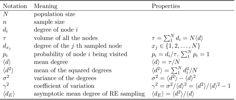
Graph # Nodes γ hdi Max degree
Twitter [41] 41,652,230 35.95 70.51 2,997,652
WikiTalk[10] 2,394,385 26.34 3.89 100,029
BerkStan[10] 685,230 14.69 19.41 84,230
EmailEu[10] 265,009 13.93 2.75 7,636
Stanford[10] 281,903 11.79 14.14 38,625
Skitter[10] 1,696,415 10.46 13.08 35,455
Youtube[42] 1,138,499 9.65 5.25 28,754
NotreDame[10] 325,729 6.40 5.25 10,721
Gowalla[10] 196,591 5.54 9.67 14,730
Epinion[10] 75,879 4.02 10.69 3,044
Google[10] 875,713 4.02 9.87 6,332
Slashdot[10] 82,168 3.35 12.27 2,552
Facebook-1[43] 2,937,612 3.14 14.27 4,356
Flickr [10] 105,936 2.65 43.43 5,425 Facebook-2 [44] 63,731 1.56 25.64 1,098
Amazon[10] 410,236 1.27 11.89 2,760
CitePatents[10] 3,774,768 1.20 8.75 793 RoadNet[10] 1,965,206 0.35 2.82 12
where hdEi is the average degree of the samples obtained by RE sampling. γ in turn
can be used to estimate the number of nodes by the following estimator [14–16]:
b
N = (γ2+ 1)n 2
2C, (2.8)
where nis the sample size, C is the number of collisions in the samples. Whenγ = 0, every node has an equal probability of being sampled and the above estimator is reduced
toNb =n2/(2C), a well-known equation in birthday paradox.
2.4
Experiments
2.4.1 Datasets
We conducted experiments on dozens of large networks we can find. Most of them are
from Stanford SNAP graph collection [10]. Due to space limitation, for some network
categories only one graph is reported if they have similar behaviour. For instance,
cita-tion graphs have similar degree distribucita-tion, similar coefficient of variacita-tion, and similar
error ratios between RN, RE, and RW sampling. For these categories, we choose only
deviates greatly from RE sampling. So we include several Web graphs, including the
Web graph on the domains of Notre Dame, Stanford, and Berkley-Stanford, to
investi-gate the cause for such deviation. Facebook data is one of the few exceptions that RE
sampling is not obviously better than RN sampling. Therefore we include two Facebook
graphs that can be found. More complete data description and programs can be found
at http://cs.uwindsor.ca/∼jlu/graph.
Altogether 18 graphs are reported and their statistics are summarized in Table2.2. They
are sorted according to γ, the coefficient of variation of the degrees. γ is proportional to the RRMSE of RN sampling, and decides whether RE is better than RN sampling.
In the last a few datasets, the maximal degrees are smaller relative to their data sizes,
causing small γ value. We highlight four datasets with italic font, whose RE sampling is not as good as RN sampling.
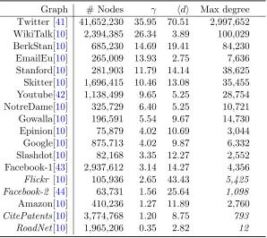
The degree distributions give an overview of the data and are shown in Figure 2.2.
Among these graphs, most of them have a long-tail distribution, resulting in large
co-efficient of variation. Graphs in the last row have small γ values because the maximal degrees are small compared to their data sizes. In particular, RoadNet graph has
max-imal degree 12. They are scale-free networks since their log-log plots obviously deviate
from straight-lines. For these graphs RE sampling does not have clear advantage. Web
graphs (sub-figures 3, 5, 8) do not form a straight line in the upper part of the
log-log plots, indicating irregularity in the graph structure. For these graphs, simple RW
sampling should be avoided.
It is interesting to note that two representative social networks Twitter and Facebook are
in the two extremes of the spectrum ofγ values, due to the way the networks are formed. Twitter allows unlimited number of followers, while Facebook has an up-limit for the
maximal number of friends. Therefore Twitter is a scale-free network with large degree
variation, while Facebook has a sharp dropping curve causing low γ value. Because of their structural difference, for Twitter data RE is hundreds of times better than RN
sampling in terms of sample size, for Facebook data RE and RN samplings are similar.
The estimators are evaluated by RRMSE (Relative Rooted MSE), which is defined as
below:
RRM SE(hcdi) =
1
hdi
v u u t
1
n
n
X
i=1
c
hdii− hdi2 (2.9)
wherehcdiis an estimator, hdiis the true average degree,hcdi
i is the estimation obtained
in the i-th run. All the RRMSE data are obtained by 5000 independent runs, except for
Twitter data that has 2000 runs due to its large size and the long computation time of
100 101 102 103 104 105 106 107
100101102103104105106107
Frequency (1)Twitter 100 101 102 103 104 105 106 107
100 101 102 103 104 105 106
(2)WikiTalk 100 101 102 103 104 105
100 101 102 103 104 105
(3)BerkStan 100 101 102 103 104 105 106
100 101 102 103 104
(4)EmailEu 100 101 102 103 104 105
100 101 102 103 104 105
(5)Stanford 100 101 102 103 104 105 106
100 101 102 103 104 105
(6)Skitter 100 101 102 103 104 105 106
100 101 102 103 104 105
Frequency (7)Youtube 100 101 102 103 104 105 106
100 101 102 103 104 105
(8)NotreDame 100 101 102 103 104 105
100 101 102 103 104 105
(9)Gowalla 100 101 102 103 104 105
100 101 102 103 104
(10)Epinion 100 101 102 103 104 105 106
100 101 102 103 104
(11)Google 100 101 102 103 104 105
100 101 102 103 104
(12)Slashdot 100 101 102 103 104 105 106 107
100 101 102 103 104
Frequency degree (13)Facebook-1 100 101 102 103 104 105
100 101 102 103 104
degree (14)Flickr 100 101 102 103 104
100 101 102 103 104
degree (15)Facebook-2 100 101 102 103 104 105
100 101 102 103 104
degree (16)Amazon 100 101 102 103 104 105 106
100 101 102 103
degree (17)Citation 100 101 102 103 104 105 106
100 101 102
degree
(18)RoadNet
Figure 2.2: Degree distributions of 18 graphs. Plots are sorted in decreasing order
of coefficient of variation γ. Graphs in the last row have small γ values because the
maximal degree is small compared to the data size. For these graphs RE sampling does not have obvious advantage. Web graphs (sub-figures 3, 5, 8) do not form a straight line in the upper part of the log-log plots, indicating irregularity in the graph structure.
For these graphs simple RW sampling should be avoided.
billions of edges that can not fit into computer memory. We use index engine Lucene
to store the data in hard drive and use search engine to mimic the random sampling
methods.
2.4.2 RE vs. RN sampling
Panel A in Figure 2.3 shows that RE outperforms RN sampling on most of the data.
The estimation error of RN sampling is proportional to γ as expected. Consequently, the figure shows that RRMSE of RN sampling grows from RoadNet up to Twitter, since
the datasets are sorted according toγ.
In contrast to the monotonic increase of RN sampling, RRMSE of RE sampling remains
mostly a constant as Theorem 2 indicates. Because of this, the RRMSE ratio between
RN and RE sampling grows almost linearly with the coefficient of variationγ as shown in panel (B) of Figure2.3. For Twitter and WikiTalk networks, RN sampling is around
15 times worse than RE sampling in terms of RRMSE. When translated into sample size,
that means 225 (= 152) times more samples are needed to produce the same confidence
interval as RE sampling.
This huge difference between RN and RE sampling will change the practice of sampling,
especially in big data. Here we are not talking about a few percentage of improvement.
(A) RRMSE of three sampling methods for 18 graphs.
0 5 10 15 20 25 30 35 40 0
5 10 15 20 25
γ
Ratio of RN and RE
0 2 4 6 8 0
1 2 3 4
(B) RRMSE ratio of RE and RN as a function ofγ.
Figure 2.3: Summary of the three sampling methods on 18 graphs. (A) Comparison
in terms of RRMSEs. (B) The advantage of RE grows as a linear function of γ. It
shows that RRMSE of RN/RE grows almost linearly withγ. Pearson’s coefficient of
correlation is 0.9354. Inset: there are four cases where RN/RE is smaller than one. These four graphs from left to right are RoadNet, Citation, Facebook-2, and Flickr. In both (A) and (B) the sample size is 400, and RRMSEs are obtained over 5000 runs
except for Twitter data that has 2000 runs.
will become even more prominent with the growth of data size. Although most data
exhibit power law distributions with similar exponent, their coefficient of variations grow
with the data size, therefore the savings of RE sampling.
There are only four datasets whose RE sampling is slightly worse than RN sampling.
Panel B in Figure2.3shows that four datasets are below the horizontal line 1. A closer
inspection on these datasets shows that they all have small degree variations as shown
in Figure2.2. RoadNetwork has maximal 12 degrees, and its degrees show a log-normal
0 2 4 6 8 RRMSE (1)Twitter 0 0.5 1 RRMSE (7)Youtube
0 500 1000 0 0.5 1 Sample Size RRMSE (13)Facebook−1 0 1 2 3 4 (2)WikiTalk 0 0.5 1 1.5 (8)NotreDame
0 500 1000 0 0.5 1 1.5 Sample Size (14)Flickr 0 0.5 1 1.5 2 2.5 (3)BerkStan 0 0.2 0.4 0.6 0.8 (9)Gowalla
0 500 1000 0 0.2 0.4 0.6 Sample Size (15)Facebook−2 0 0.5 1 1.5 2 (4)EmailEu 0 0.2 0.4 0.6 (10)Epinion
0 500 1000 0 0.1 0.2 0.3 Sample Size (16)Amazon 0 0.5 1 1.5 (5)Stanford 0 0.2 0.4 0.6 (11)Google
0 500 1000 0 0.2 0.4 0.6 Sample Size (17)Citation 0 0.5 1 1.5 (6)Skitter 0 0.2 0.4 0.6 (12)Slashdot
0 500 1000 0 0.05 0.1 0.15 Sample Size (18)RoadNet
Figure 2.4: RRMSEs of RN, RE, and RW samplings as a function of sample size for
18 graphs. The dotted, dashed, and solid lines are for RN(. . .), RE(−−), and RW(–)
samplings respectively. It shows that in most cases the sample size does not change the relative positions of the sampling methods. The exceptions are the web graphs 3 and 5 where RW sampling does not improve with the increase of sample size because of the
random walk traps.
100 105 100 102 104 (2)WikiTalk 100 105 100 101 102 103 (3)BerkStan 100 102 104 100 102 104 (4)EmailEu 100 105 100 101 102 103 (5)Stanford 100 105 100 101 102 103 (6)Skitter
100 105 100 101 102 103 Frequency (7)Youtube
100 105 100
101 102 103
(8)NotreDame
100 105 100
101 102 103
(9)Gowalla
100 102 104 100
101 102 103
(10)Epinion
100 102 104 100
101 102 103
(11)Google
100 102 104 100 101 102 103 (12)Slashdot 100 102 104 100 101 102 103 Degree Frequency (13)Facebook−1 100 102 104 100 101 102 103 Degree (14)Flickr 100 102 104 100 101 102 Degree (15)Facebook−2 100 102 104 100 102 104 Degree (16)Amazon 100 102 104 100 101 102 103 Degree (17)Citation 100 100 102 104 Degree (18)RoadNet
Figure 2.5: The degree distributions of the samples obtained from RE (Random
abnormally small compared with its size. Flickr has an irregular degree distribution that
has a large bump around degree 100.
Another perspective to understand the reduced variance of RE sampling is its sample
distributions in Figure2.5, where the sample size 8000. It shows that most of the sample
distributions have a “V” shape, indicating that the small nodes still follow power law
roughly as in the original data, while the large nodes can be sampled many times. In
other words, both small and large nodes are sampled multiple times but for different
reasons. Small nodes are sampled because there are many of them. Although each
individual small node has a very small probability of being sampled, collectively the large
number of small nodes will guarantee that some will be sampled. On the other hand,
large nodes are sampled because they have higher probability of being hit by random
edges, even though there are only a few of them. Therefore both small and large nodes
are well represented in the sample, resulting in small variance of the estimation. In RN
sampling, large nodes are included by chance, inducing a large variance in estimation.
The datasets that do not have the “V” shape in RE sampling happen to be the ones not in
favour of RE sampling. They do not have the long tail, do not have very large nodes, and
do not have large nodes that are sampled many times. Their RE sample distributions are
just similar to the original data, or to RN sample distribution. Therefore RE sampling
does not have an advantage in this kind of data.
Two of the representative online social networks are Twitter and Facebook. It is
in-teresting to see that they favour different sampling methods, one RE sampling and the
other RN sampling. Moreover, their RN/RE ratios happen to be on the two extremes of
the spectrum. Twitter has the second highest RN/RE ratio because it is scale-free and
the largest network in our experiment. Facebook-2 has the lowest RN/RE ratio because
it has a cap on the number of friends.
2.4.3 RW vs. RN sampling
In many practical situations, RE sampling is not easy to implement, while RW sampling
is supported by most real networks such as Twitter. RW sampling can be regarded as
an approximation to RE sampling in thatasymptoticallythe node sampling probability is proportional to its degree. The difference between RW and RE is dependent on the
mixing time, the steps to reach closely enough the stationary distribution. The mixing
time, in turn, is inversely proportional to the square of the conductance of the graph
V is
Φ(S) =
P
i∈S,j∈V\SAij
min(A(S), A(V\S)) (2.10)
where A is the adjacency matrix of the graph, and A(S) =P
i∈S,j∈V Aij. The
conduc-tance of the graph is
Φ =minSΦ(S). (2.11)
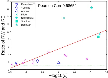
Our experiments as depicted in Figure 2.3(A) show that RW is worse than RE
consis-tently as expected. To have a detailed comparison between RW and RE samplings,
Fig-ure2.6plots the ratio of RRMSEs (RW/RE) against graph conductance for 18 datasets.
The sample size for both RN and RW samplings is 400, and each RRMSE is obtained
from 2000 runs. It shows that all the ratios are above the dashed green line for the value
of one, indicating RE is always better than RW. When the conductance is not very small
(the left section of the plot), overall RW can approximate RE sampling well, thereby
outperforms RN sampling. When the conductance is small, indicating the existence
of loosely connected components, RW can be dramatically worse than RE. The ratio
RW/RE can be as large as that of RN/RE, thereby offsets the advantage gained by PPS
(probability proportional to size) sampling, making RW and RN incomparable. Taking
NotreDame and Flickr are example, their RW samplings are around 15 times worse than
RE sampling in terms of RRMSE. When measured in sample size, they can be 152 = 225
times worse. This reveals the reason why there are mixed results for the comparison
between RW and RN samplings. Both RN and RW can be 10 times worse than RE,
but for different reasons. RN is worse because of the large degree variance, while RW is
because of the existence of loosely connected component indicated by small conducatnce
Φ. It is remarkable that both degree variance and loosely connect component can be
the dominant factor.
To find out the reason for the poor performance of RW sampling for some datasets,
we plot the random walk traces in Figure 2.7 for six networks. Three of them (Flickr,
NotreDame, and Stanford) have low graph conductance, while three others (Facebook,
Amazon and Youtube) have high conductance as comparison. These six networks are
also highlighted in Figure 2.6 using different markers. Figure 2.8 shows the
conduc-tances over the size of the subcomponents. For the networks in the first row, their
lowest conductance are smaller than 10−3. For Flickr data, the conductance value dips
down only when the component size is large (≈ 104). This is reflected in its random
walk trace where there are two components clearly separate by a long single edge link.
1.5 2 2.5 3 3.5 4 4.5 0
2 4 6 8 10 12 14 16 18
−log10(φ)
Ratio of RW and RE
Pearson Corr:0.68652
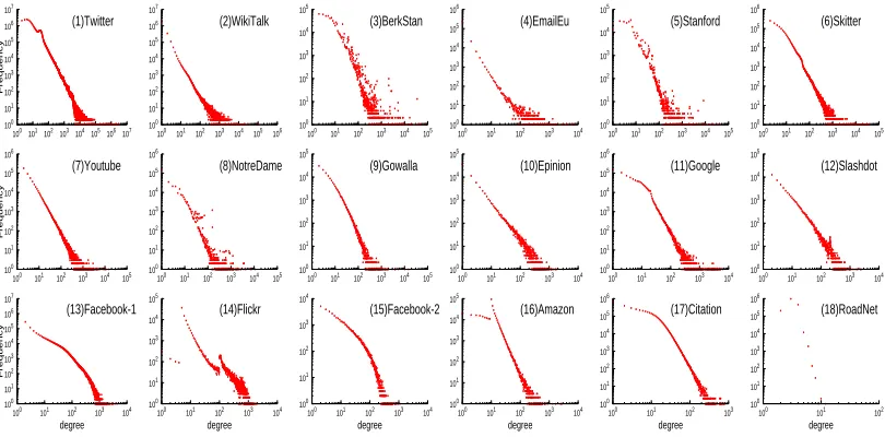
Facebbok−2 Youtube Amazon Flickr NotreDame Stanford BerkStan
Figure 2.6: Standard error ratio between RW and RE vs. graph conductance Φ for
18 datasets. Sample size is 400.
many low conductance values over a variety of component sizes. Those three networks
are in contrast to the well enmeshed networks Facebook-2 and Youtube, whose the
con-ductances are high. Amazon also has a low conductance (≈ 10−3), but reaches the
lowest point only when the component size is around 100. This small component has
less impact on the overall network structure as shown in the RW trace, and little impact
on the performance of RW as shown in Figure2.6.
2.5
Conclusions
This paper shows the importance of selecting the appropriate sampling method –the
difference between the sampling methods can be infinitely large in theory and orders
of magnitude in observed data. Such a large difference will have great impact on the
sampling practice, especially for web-based networks such as online social networks where
the sampling process is costly because of network traffic and daily quota.
It is remarkable to notice that it is uniform random node (RN) sampling that is on the
downside of the comparison. In the past, great efforts are devoted to obtain uniform
random samples using methods such as Metropolis-Hasting Random Walk [7]. During
the sampling process many nodes are visited, examined, and rejected. In the end these
precious uniform random samples can be much worse than the samples obtained using
low cost simple random walk that are supported by many online data sources.
RN sampling is not always inferior to RW or RE sampling. When the data has a normal
distribution RN sampling should be the method of choice. When the network is large
Flickr NotreDame Stanford Web
100~+
∞
10~99
2~9
1
Amazon Facebook-2 Youtube
Figure 2.7: (Best viewed in colour) Random walks on six networks. Flickr,
NotreDame and Stanford have loosely connected components while Amazon, Facebook
and Youtube are well enmeshed. Each random walk contains 6×10⁴ nodes except
NotreDame which has 15×104 nodes. Node colour indicates the degree of the node.
Green=1; Blue=2∼9; Yellow=10∼99; Red=100+.
10-4 10-3 10-2 10-1 100
100 101 102 103 104 105
Conductance
Number of nodes in the cluster Flickr 10-5 10-4 10-3 10-2 10-1 100
100 101 102 103 104 105 106
Conductance
Number of nodes in the cluster NotreDame 10-5 10-4 10-3 10-2 10-1 100
100 101 102 103 104 105 106
Conductance
Number of nodes in the cluster Stanford 10-4 10-3 10-2 10-1 100
100 101 102 103 104 105 106
Conductance
Number of nodes in the cluster Amazon
10-2 10-1 100
100 101 102 103 104 105
Conductance
Number of nodes in the cluster Facebook-2
10-3 10-2 10-1 100
100 101 102 103 104 105 106
Conductance
Number of nodes in the cluster Youtube
Figure 2.8: Conductance Φ(S) over |S|, the size of the the components, for six
For data not following some distribution exactly, we suggest to useγ, the coefficient of variation of the degrees, to select the sampling method. While it is easy to understand
that uniform random sampling has large estimation error for data with large variance,
it is not straightforward to see whether RE sampling can reduce the variance for data of
various distributions. We show that the estimation error of RE sampling varies slightly
across all the data we examined.
Although we have a clear answer for the selection of sampling methods between RN
and RE samplings, RE sampling may not be supported in some real applications. RW
sampling is a more practical method that can approximate RE sampling in that both
methods sample nodes with probability proportional to its size. The difference is that
in RW sampling this is true only asymptotically. Thus the performance of RW sampling
differs from data to data. Our experiments show that in general RW sampling performs
a little bit below RE sampling as expected, but sometimes it can be much worse, even
worse than RN sampling when there are loosely connected components in the graph
characterized by graph conductance.
This paper focuses on average degree estimation so that the detailed analysis and
com-parison could be done. It is the first building block on top of which other properties
could be derived. For instance, population size estimation is built on top of average
degree estimation as shown in Section 2.3.4. In addition to the degrees sampled, size
estimation depends on the collisions observed. This additional dimension of variation
makes the evaluation of the sampling methods not so straightforward.
Overall, we study the most basic sampling methods for the simplest property of a graph
so that we can draw conclusive results. Based on this result, we can develop more
advanced sampling methods for more complex properties. For sampling methods, with
the understanding that RE sampling is the best for scale-free networks, we can design
a sampling method that can approximate RE sampling as much as possible, such as
random walk with restart. For graph properties to be estimated, we can also discover
friends of friends and Gini coefficient in addition to population size [16], and we expect
that RE sampling would be better for some other structural graph properties such as
clustering coefficient.
2.6
Acknowledgements
This research is supported by NSERC (Natural Sciences and Engineering Research
2.7
Appendix
Both Theorem 1 and Theorem 2 assume that the degrees follow the Zipf’s-Mandelbrot
law [39] which states that if the degrees di are sorted in descending order, then
di=
A
α+i, (2.12)
whereα and A are constants. αN. All the degrees sum up toτ, i.e.,
N
X
1
di ≈
Z N
1
A
α+xdx≈Aln( α+N
α+ 1) =AlnB =τ, (2.13)
where we useB = (α+N)/(α+1) to make our derivations more concise. The normalizing constantA=τ /lnB. Besides,PN
1 d2i can be approximated by the following since N is
a very large number:
N
X
i=1
d2i ≈
Z N
1
A2
(α+x)2dx≈
A2
α+ 1. (2.14)
2.7.1 Proof of Theorem 1
Proof. Based on Equations 2.13 and 2.14, the variance of all the degrees is
σ2 =hd2i − hdi2=hdi2
"
N
PN
1 d2i
(PN
1 di)2
−1
#
≈ hdi2
N
(α+ 1) ln2B −1
. (2.15)
Using central limit theorem,
var(hcdi
RN) =
σ2 n =
hdi2
n
N
(α+ 1) ln2B −1
. (2.16)
2.7.2 Proof of Theorem 2
Proof. When nodes are sampled with simple random walk, the asymptotic probability
of the node i being visited is pi =di/ τ. When n nodes (x1, x2, . . . , xn) are sampled,
N is [38]:
b
NH =
1 n n X i=1 1
pxi
= τ n n X 1 1
dxi
, (2.17)
and the variance of NdH is [38]:
var(NdH) =
1 n N X i=1 pi 1 pi −N 2 . (2.18)
Replacing pi with di/τ and expandingdi with A/(α+i), we have
var(NdH) =
1 n τ A N X 1
i−N2
! ≈ N 2 n lnB
2 −1
. (2.19)
The Taylor expansion of hcdi
RE aroundN is
c
hdiRE = τ
d
NH
=τ 1
N −
d
NH−N
N2 +. . .
!
. (2.20)
By the Delta method, the variance ofhcdi
RE is
var(hcdiRE) =τ2
var(NdH)
N4 =
hdi2
n
lnB
2 −1
Uniform Random Sampling not
Recommended for Size
Estimation
This paper was submitted as:
Hao Wang, Jianguo Lu,Uniform Random Sampling not Recommended for Size
Estima-tion. Physica A: Statistical Mechanics and its Applications, 2013, submitted.