ARJUN, VINOD. A Database Level Implementation To Enforce Fine Grained Access Control. (Under the direction of Dr. Ting Yu).
by Vinod Arjun
A thesis submitted to the Graduate Faculty of North Carolina State University
in partial fullfillment of the requirements for the Degree of
Master of Science
Computer Science
Raleigh, North Carolina
2008
APPROVED BY:
Dr. Peng Ning Dr. Rada Chirkova
Dr. Ting Yu
DEDICATION
BIOGRAPHY
ACKNOWLEDGMENTS
I would like to sincerely thank my advisor Dr. Ting Yu for his guidance. I thoroughly enjoyed working with him on this thesis topic. I cannot thank him enough for his constant motivation and support. His comments and suggestions were invaluable in improving the content of this thesis. I would also like to thank Dr. Rada Chirkova and Dr. Peng Ning for taking time off from their busy schedule and agreeing to serve on my thesis committee.
TABLE OF CONTENTS
LIST OF FIGURES . . . vi
1 Introduction . . . 1
1.1 Enforcing Fine Grained Access Control . . . 1
1.2 Our Contribution . . . 4
2 Related Work . . . 6
2.1 Basic Concepts of Access Control . . . 6
2.2 Specification of Privacy Policies . . . 10
2.3 Enforcement of Privacy Policies . . . 13
3 A Sound and Secure Query Evaluation Algorithm to Enforce Fine Grained Access Control . . . 18
3.1 Correctness Criteria . . . 18
3.1.1 Sound . . . 19
3.1.2 Secure . . . 20
3.1.3 Maximal . . . 22
3.2 A Labeling Mechanism for Masking a Database . . . 22
3.3 A Sound and Secure Approach to Query Evaluation . . . 25
4 A Database Level Implementation to Enforce Fine Grained Access Con-trol . . . 29
4.1 Assigning Modes of Evaluation to Sub-Queries . . . 30
4.2 Implementing Aggressive and Conservative Minus . . . 31
4.2.1 Straightforward Approach to Implement Aggressive and Conservative Minus . . . 32
4.2.2 An Indexed Approach to Implement Aggressive and Conservative Minus 32 5 Experimental Results and Analysis . . . 49
5.1 Experimental Setup . . . 50
5.2 Results and Analysis . . . 51
5.3 Discussion . . . 61
6 Conclusions and Future Work . . . 63
6.1 Conclusions . . . 63
6.2 Future Work . . . 64
LIST OF FIGURES
Figure 1.1 Application Level Access Control [1] . . . 2
Figure 1.2 Database Level Access Control [1]. . . 2
Figure 2.1 Trojan Horse Attack [3] . . . 7
Figure 2.2 MAC preventing Trojan Horse Attack [3] . . . 8
Figure 2.3 Access Control Matrix [3] . . . 9
Figure 2.4 Access Control List [3] . . . 9
Figure 2.5 Capability List [3] . . . 10
Figure 2.6 Fine Grained Restriction Syntax [15] . . . 12
Figure 2.7 Oracle’s Virtual Private Database Approach [10] . . . 14
Figure 3.1 Example to illustrate why existing approaches are not sound . . . 20
Figure 3.2 Example to illustrate labeling mechanism . . . 24
Figure 3.3 Sound and Secure Query Evaluation Algorithm [5] . . . 26
Figure 3.4 Query Modification Approach [5] . . . 28
Figure 4.1 Generic Form of the ”Bucket” structure . . . 35
Figure 4.2 Example to demonstrate building of ”Bucket” structure . . . 37
Figure 4.3 Example to illustrate computation of aggressive minus . . . 39
Figure 4.4 Logical View of ”Bucket” Structure in disk . . . 43
Figure 4.5 Example illustrating storage of ”Bucket” structure in disk . . . 44
Figure 4.6 Example to illustrate performance of on-demand and prefetching schemes . . 47
Figure 5.2 Comparison of SoundDB, SoundQM and Unmodified approaches. Other pa-rameters: Range = 1000, Sensitivity = 2, Disclosure Probability = 75% . . . 52
Figure 5.3 Break up of SoundDB into index building and query evaluation. Other pa-rameters: Range = 1000, Sensitivity = 2, Disclosure Probability = 75% . . . 52
Figure 5.4 Behavior of SoundQM with varying Range. Other parameters: Sensitivity = 2, Disclosure Probability = 75% . . . 53
Figure 5.5 Behavior of SoundDB with varying Range. Other parameters: Sensitivity = 2, Disclosure Probability = 75% . . . 54
Figure 5.6 Behavior of SoundQM with varying Disclosure Probability. Other parameters: Sensitivity = 2, Table Size = 100000, Range = 1000 . . . 55
Figure 5.7 Behavior of SoundDB with varying Disclosure Probability. Other parameters: Sensitivity = 2, Table Size = 100000, Range = 1000 . . . 55
Figure 5.8 Number of Tuples inT1 having a match in sub-buckets corresponding to the NULL bucket in the ”‘Bucket”’ structure of T2 vs Disclosure Probability. Other parameters: Sensitivity = 2, Table Size = 100000, Range = 1000 . . . 56
Figure 5.9 Comparison of prefetching and ondemand schemes of SoundDB approach. Other parameters: Sensitivity = 1, Disclosure Probability = 0%, Sensitive Attribute = VA, Range = 1000 . . . 57
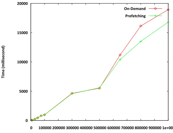
Figure 5.10 Comparison of prefetching and ondemand schemes of SoundDB approach. Other parameters: Sensitivity = 1, Table Size = 1000000, Sensitive Attribute = VA, Range = 1000. . . 59
Figure 5.11Performance difference between prefetching and ondemand schemes of SoundDB approach. Other parameters: Sensitivity = 1, Table Size = 1000000, Sensitive At-tribute = VA, Range = 1000 . . . 59
Figure 5.12Performance of SoundDB prefetching scheme with varying amounts of system memory. Other parameters: Sensitivity = 2, Disclosure Probability = 75%, Table Size = 1000000, Range = 1000 . . . 60
Chapter 1
Introduction
As privacy protection has gained significant importance, organizations have been forced to protect individual preferences and comply with many enacted privacy laws. This has been a strong driving force for access control in databases. For example, in a typical bank setting, the bank database would contain the account information of many customers. When one customer tries to view his account details it is imperative that he view only his account information and not of any other customers’. The primary means of achieving this requirement is by enforcing appropriate access control.
Much work has been done on the specification of database access control policies [13, 15, 16]. Traditional policies treat tables or columns as the basic access control unit. Re-cently, security policy models have emerged to specify row-level or cell-level access control. Conceptually, with fine-grained access control, a policy defines for each cell whether it can be accessed by a user. In this thesis we focus on enforcing access control policies while evaluating a query issued by the user. We assume that the access control policies for each user are already in place. Hence, we do not focus on the specification of such policies.
1.1
Enforcing Fine Grained Access Control
cells are accessed by the query, thus enforcing the access policies for that user. The rewritten queryQ0 is passed on to the DBMS for execution.
User Issues Query Q
Middleware Rewrites Query Q
to Query Q’ Enforcing Access
DBMS Executes Query Q’
Q y Q g
Control Query Q
Figure 1.1: Application Level Access Control [1]
In this approach the underlying DBMS need not be changed. It is required only to write the middleware between the user and the DBMS in order to rewrite the query to enforce access control. It is easy to deploy in existing systems. On the other hand, the rewritten queries can be too expensive to execute. In addition, if the user has direct access to relations in the DBMS then he can bypass the middleware that rewrites the query, in which case the access policies do not get enforced [5].
In the second approach, access control is placed at the database level, as shown in Fig-ure 1.2. In this approach, the query Q that the user issues does not get rewritten by a middleware as in the first approach. Instead, the DBMS receives and executes the queryQ taking into account the access control policies formulated for the issuer of the query.
User Issues
Query Q Middleware
DBMS Executes Query Q Taking into Account the Access Control P li i S ifi d Policies Specified
for the User
Figure 1.2: Database Level Access Control [1]
when they get integrated into the DBMS. The major drawback with this approach is that the underlying DBMS would have to be changed to support access control [5].
Some of the existing approaches to enforce fine grained access control include Oracle’s Virtual Private Database [7], query modification in INGRES [8], access control in DB2 [9], and work in Hippocratic Databases [6]. How do we actually know that the results obtained by these query evaluation algorithms enforcing access control are indeed correct? Recently, Wang et al. [5] have proposed three correctness criteria that an ideal query evaluation algorithm enforcing fine grained access control should possess, namely, sound, secure and maximal. The algorithm is sound if the answer returned by it is consistent with the answer when there is no fine-grained access control. The algorithm is secure if the returned answer does not leak information not allowed by the policy. The algorithm is maximal if it returns as much information as possible, while satisfying the first two properties. In addition to the above stated three properties, the algorithm should be scalable, i.e. be able to handle databases of arbitrary size.
Unfortunately, none of the existing approaches satisfy all the correctness criteria proposed by Wang et al [5]. They argue that the existing approaches do not strive to achieve the maximal property. To appreciate this argument let us assume that there are two tables that are linked through an attributeA. IfAis considered sensitive, then the existing approaches replace the cells inAwith NULL value. As a result, it becomes impossible to maintain the association between the two tables. They also argue that the exisiting approaches violate the soundness property. They attribute this to the way in which existing approaches evaluate the SQL set difference operation. We encourage the readers to see the example in Section 3.1.1 to appreciate this argument.
for queries involving SQLset difference operation, which have been discussed in Section 3.3. They have implemented their algorithm using a query modification approach.
Though their query evaluation algorithm was novel, Wang et al. were not able to show good performance through their query modification approach. For moderately sized tables having 50000 and 100000 records, their approach takes about 8 and 32 seconds to evaluate queries involving SQLset difference operation. For time critical applications this is not fast enough. Also, their approach does not scale well with tables of larger sizes. Thus, there is scope for further research in this area and this has precisely been the motivating factor for this thesis.
1.2
Our Contribution
• We have implemented a query evaluation algorithm that enforces fine grained access control at the database level. We have chosen to modify the query evaluation en-gine of POSTGRESQL, which is an open source database management system, to incorporate the access control features. In this way, the overhead that is involved in query rewriting is overcome. Though the task of incorporating access control into the DBMS is difficult, the performance increase compared to the query rewriting approach is substantial, as can be observed from the graphs in chapter 5.
• We have come up with a few optimizations to improve the performance of the database level implementation. We have used an index structure, which has been discussed in chapter 4, to efficiently evaluate queries involving SQLset difference operation.
• Another challenging issue that we have addressed is that of scalability. When relations of arbitrarily large sizes are used in queries, then memory management becomes an important issue. The main memory might not be sufficient enough to hold the entire relation, in which case we might have to turn to the secondary disk as an alternative. Our implementation tries to make use of the main memory in an adaptive fashion, i.e. try to use as much main memory as available. We have also tried out a few optimizations in this regard, which are discussed in chapter 4.
Wang et al. [5]. The experimental results, which are presented in chapter 5, conclu-sively show that our database-level implementation to enforce access control presented in this thesis performs substantially better compared with the query modification ap-proach. In fact, the results presented in chapter 5 show that the performance of the DBMS with access control implemented within it is comparable to the original imple-mentation of the DBMS that has no access control features. This implies that it is not too expensive to incorporate access control within DBMSs and hence is practical.
Chapter 2
Related Work
The work presented in this thesis is related to access control, privacy policy specifi-cation and access control enforcement. We first discuss the basic concepts of access control. Towards this end, we first discuss the modeling of access policies and then elaborate on modeling the system state that is relevant to access control. We then discuss the existing work with regard to specification of access control policies in DBMS. Finally, we discuss some of the most relevant work in enforcing access control policies in DBMS.
2.1
Basic Concepts of Access Control
Two major ways to model access control policies include Discretionary Access Control (DAC) and Mandatory Access Control (MAC).
file into a new file called ”chapter1.doc” and gives his friend Carol read and write accesses to the file. Thus, Carol, who isn’t registered for the CSC574 class, gets access to the file that she isn’t supposed to. For this reason, the DAC scheme is subject to Trojan Horse attacks. Figure 2.1 illustrates the typical way a Trojan Horse attack is carried out.
File F Principal A
executes A: r
ACL
Software Game Trojan Horse
File F
read A: w
B File G
write B: r
A: w
Figure 2.1: Trojan Horse Attack [3]
In the scenario depicted in Figure 2.1, user B wants to know the contents of file F for which she does not have read access. User A has read and write access to file F. In this situation, B embeds a Trojan Horse program into a program that A trusts, like a software game, and entices A into executing it. Also, B creates another file G, gives read access to herself and write access to A. When A plays the game thus executing it, the Trojan Horse program embedded within the game can access the contents of file F since it is running on behalf of A. Now, it copies the contents of file F into file G due to the permissions granted to A on file G. Hence, B can now read the contents of file F that has been copied into file G. Clearly, the DAC scheme has a weakness against Trojan Horse attacks. The MAC scheme, which is discussed subsequently, is designed to overcome this drawback.
In the MAC scheme, access control policies are formulated centrally by system adminis-trators. The access of subjects to objects is restricted through the introduction of security labels. The data objects are assigned classification levels such as Top Secret, Secret, Un-classified etc., and each user is assigned a clearance level. The following two restrictions for access control are adopted in the MAC scheme [4].
• Star Property: Subject S can write object O only if the security label of O dominates the clearance level of S. Intuitively, this restriction vouches for ”no write down”.
The Star Property stated above enables the MAC scheme to overcome the Trojan Horse attacks, as elaborated in Figure 2.2.
File F Principal A
executes A: r
ACL
Software Game Trojan Horse
File F
read A: w
B File G
write B: rA: w
Figure 2.2: MAC preventing Trojan Horse Attack [3]
As shown in Figure 2.2, when principal A executes the program containing the Trojan Horse, the program can read the contents of file F since the program, executing on behalf of A, has the required permissions to do so. The program is prevented from writing the contents of file F into file G as this would otherwise violate the Star Property. Hence the Trojan Horse attack is thwarted. The MAC scheme is used for highly secure systems such as military applications, but turns out to be inappropriate when it comes to governmental and industrial environments where a lot if information is unclassified, but sensitive. Role-Based Access Control (RBAC), which is discussed subsequently, is used in such environments.
In the RBAC scheme [2], the system administrator assigns permissions to roles. When a user assumes a particular role, she would inherit the permissions that go with that role. Roles in an organization would fall into a neat hierarchy. Often, roles within the organiza-tions remain fixed, but, the role that a user assumes varies from time to time depending on what job the user has to accomplish. Generally, the principle of least privilege has to be followed while assigning roles to the user. It is required that the user be given no higher privilege than what is needed to perform the job.
System state relevant to access control can be modeled as a matrix as shown in Figure 2.3. The rows of the matrix correspond to the various subjects. Subjects can be principals, or programs executing on behalf of the principals. The column of the matrix represents objects. Objects are anything on which subjects can perform operations, such as file, directory, memory segments etc., or they can be subjects too with operations like kill, suspend etc. The cells specify the access of the subject to the object.
Objects (and Subjects)
r w r
U
F G
Objects (and Subjects)
S
u r w
own
r
r w
U V u b j e c own V t s
Figure 2.3: Access Control Matrix [3]
Access Control Matrices are not efficient to represent system state pertaining to access control. This is because, very often, they are sparsely populated, as a result of which too much space gets wasted. There are two alternatives to the matrix modeling, namely, Access Control List (ACL) and Capability List.
U: r U: w U: own F U: r V: r V: w G V: own
Figure 2.4: Access Control List [3]
all the subjects that have access rights on a given object, and is also easy to revoke all the subject’s access rights on a given object, but, it is hard to revoke all the access rights of a given subject. This is because, to revoke all the access rights of a given subject, it is required to scan the ACLs of all the objects.
F/r, F/w, F/own, G/r U
G/r G/w G/own V G/r, G/w, G/own V
Figure 2.5: Capability List [3]
In Capability Lists, each row of the access matrix is stored along with the access permis-sions to objects appearing in that row. Figure 2.5 shows the Capability Lists of two subjects U and V. It indicates that the subject U has read permissions on both objects F and G. In addition, U has write and own privileges on object F. Subject V has read, write and own privileges on object G. Capabilities provide for superior access review on a per-subject basis, but, it is hard to revoke all the access permissions on a particular object [3].
2.2
Specification of Privacy Policies
The GRANT command in SQL [13] can be used to specify access restrictions at the table or relation level. When a user creates a new table, then he is entirely responsible for that table, and he can give privileges to whomever he wishes to. The privileges that the user can grant on a table include the ability to use that table in a query (READ), and ability to perform INSERTs, UPDATEs and DELETEs on the table. The syntax for the GRANT command is as follows.
GRANT {All Rights/<privileges>/All but<privileges>} ON <table> TO<user-list> [WITH GRANT-OPTION]
grant their privileges on the table to other users. For example, let’s suppose that user Alice creates a table named ”ExamSchedule” to maintain the semester exam schedules. She, being helpful, decides to give her friend Bob the privilege to read from the table so that he too can benefit from it. In addition, she decides to give Bob the privilege to grant to other students hoping that other students too would make use of it. In order to accomplish this task, she issues the following GRANT statement.
Alice: GRANT READ ON EXAMSCHEDULE TO Bob WITH GRANT-OPTION
Griffiths et al. [14] extended this approach to handle conflicts that could possibly arise when multiple users grant conflicting privileges on a table to other users. They have done significant work in handling privilege revocations. One major observation to be made here is that the GRANT command of SQL allows a user to grant privileges at the table or relation level. However, this approach isn’t sufficient enough to handle very complex privacy policies that are prevalent these days. There is a necessity for a scheme to specify access control policies at a more fine-grained level.
In their work on Hippocratic databases, Agarwal et al. [16] have specified access control in a ”table-format”. Their approach can be used to specify access control policies easily at the column level. For each purpose and for each attribute (column) accessed for that purpose, they identify the external recipients (whom the information can be given out to), the retention period (how long the information is stored), and the authorized users (those who can access this information). This is captured in two tables, namely, privacy-policies and privacy-authorizations. The schemas for the two tables are as follows.
Privacy-Policies (purpose, table, attribute, external recipients, retention)
Privacy Authorizations (purpose, table, attribute, authorized users)
Agarwal et al. [15] have provided access control constructs to specify access restrictions at the column level, row level and cell level. Figure 2.6 depicts the syntax, as defined by Agarwal et al., for specifying access restrictions. It states that those belonging to auth-name-1 list, but not belonging to auth-name-2 list, have restricted access on table-x. The restrictions can be specified at the column level by providing the list of columns to which the restriction applies, or at the row level by providing some search-condition in the WHERE clause or at the cell level by combining the restrictions at the row and column level. The syntax also allows the specification of a purpose, which determines the way the query result is going to be used, and recipient, which determines the users who would be using the query result. The restriction can be applied to any or all of select, insert, update and delete statements. Agarwal et al. have provided means to combine multiple restrictions that may be defined for a single user on a single table. In such a scenario, multiple restrictions can be combined using intersection or union operation. In the intersection approach, the user is allowed to access data that is defined by the intersection of the restrictions, thus reducing the user’s access when more restrictions are added. In the union approach, the user is allowed to access data that is defined by the union of all the applicable restrictions, thus giving the user more access when restrictions are added.
create restrictionrestriction-name
ontable x
ontable-x
forauth-name-1 [exceptauth-name-2] ( ( (to columnscolumn-name-list)
| (to rows[wheresearch-condition])
| (to cells(column-name-list [wheresearch-condition])+) )
[for purposepurpose-list] [for recipientrecipient-list] )+
command restriction command restriction
Figure 2.6: Fine Grained Restriction Syntax [15]
or location. In spite of these limitations, this method can be very effective in restricting access to data at column, row or cell level.
2.3
Enforcement of Privacy Policies
Traditionally privacy policies were enforced in relational databases through views. Let’s suppose there exists a relation named ”Student” with attributes Student Id, Name, Date of Birth, and CGPA, and the privacy policy states that every student is allowed to view his details alone and should not be able to view records corresponding to any other students’. In this scenario, the system administrator would have to create views for each of the students. For example, if we assume that the ”Student” relation contains a record corresponding to Student-Id 1001, then the view would be manually created as follows.
CREATE VIEW Student1001 as SELECT Student Id, Name, Date of Birth, CGPA from Student WHERE Student Id = 1001;
The same thing would have to be repeated for each student, replacing the view name and the student id present in the WHERE clause. Once the views have been created, the system administrator would have to grant permissions for each user to access his view. One major drawback is that this approach isn’t scalable with the increase in number of users. Also, minor modifications in privacy policies would lead to the manual creation of a number of additional views. These limitations make the trivial view based approach unsuitable for enforcing access control policies.
algorithm fails to specify clearly the manner in which operators such as set difference need to be handled, which apparently requires special treatment. If while handling the set difference operator, the algorithm treats the ”incomplete” or ”hidden” information as ”NULL”, then it fails to obey the soundness property. This has been explained with example in chapter 3.
Oracle’s Virtual Private Database (VPD) approach [10], which is yet another query mod-ification approach, overcomes the drawbacks of the trivial view based approach by dynam-ically modifying the queries issued by the users in order to enforce access control as shown in Figure 2.7. In the scenario depicted in Figure 2.7, two users, one with an id of ’10’ and another with an id of ’20’, try to access the ”ORDERS” relation. The privacy policies formulated by the database administrator allows the user with id ’10’ to access his record alone, but does not allow the user with id ’20’ to access the relation. Now, when the user with id ’10’ issues a select query over the ”ORDERS” relation, the Oracle server dynami-cally generates a predicate, that is a ’where’ clause and appends it to the user query, thus modifying the query transparently to the user. When the modified query is issued against the relation, the result contains the record pertaining to the issuer of the query. In the sec-ond case, when the user with id ’20’ issues the select query, the server, as before, appends the predicate generated to the query. Since the issuer does not have access to the relation, as reflected by the predicate generated, the result returned is NULL.
SELECT * FROM
where terr_id = 10;
Oracle 9i ORDERS;
where terr_id = 20;
Figure 2.7: Oracle’s Virtual Private Database Approach [10]
information is used by the policy functions to generate predicates for different users. One major drawback with this dynamic query modification approach is that the predicates that are appended to the user issued query can be complex, for example, they can be sub-queries by themselves. In that case, the execution time of the modified query can greatly increase.
The column level VPD [7] allows one to enforce row-level security when a column that is considered sensitive is used in a query. It has two modes of operation, one is a default behavior and the other is a column masking behavior. In the default behavior, the number of rows returned as result is restricted. In the masking behavior, all rows are displayed, but the sensitive columns are replaced with NULL values. As pointed out by Wang et al. [5], the default behavior violates the ”maximality” criteria, and the column masking behavior violates the ”soundness” property, both of which have been briefly discussed about in chapter 1. It is explained in detail with an example in chapter 3 as to why the soundness property is violated when incomplete data is treated as ”NULL” value. A more formal definition of the correctness criteria can be found in chapter 3.
In addition to the above listed drawbacks of Oracles’ VPD approach, as pointed out by Rizvi et al. [11], quite often the results returned by this approach can be misleading to the user. For example, if a student issues a query to a ”Student” relation to obtain the average grade for a particular course, and the privacy policy allows the student to access only his own record, then the average grade returned would be the student’s grade itself. Thus, the student is misled into believing that his grade is the average grade of the class in that particular course.
CREATE AUTHORIZATION VIEW MyRecord as SELECT StudentId, Name, CGPA from Student WHERE StudentId = $userid;
$userid appears as a parameter in this view definition. Thus, this single view definition would suffice for all the students. Based on the privacy policies established, multiple au-thorization views could possibly be defined for each user. Rizvi et al. try to validate the query before actually executing it. In order to do so, they determine if the issued query can be answered based on the authorization views associated with the issuer. If it’s possible to do so, then they execute the query unmodified over the appropriate authorization view and return the result, else they reject the query. By rejecting the query, they violate the ”maximality” criteria [5].
Bond et al. [9] used a label based approach to enforce access control in DB2. The concept of security label is central to the label based access control scheme. As defined in IBM’s document [12], a security label component is defined as ”a database object that represents a criterion you want to use to determine if a user should access a piece of data”. For example, in order to view the grades of all students in a course, the criterion could be that the user is an instructor or a teaching assistant for that course. A security policy describes the criteria that will be used to decide who has access to what data. When the security policy is in place, security labels, which are a collection of security label components, can be associated with cells in a relation to protect it. If the user needs to access data in a particular cell, then he must obtain the appropriate security label from the database administrator, which is also called a credential. When a user tries to access protected data, that user’s security label is compared to the security label protecting the data. If the user has no access to that column, then an error message is flagged. If the user has no access to the row in which the data is present, then those rows are hidden from the user, violating ”soundness” and ”maximality” principle.
Chapter 3
A Sound and Secure Query
Evaluation Algorithm to Enforce
Fine Grained Access Control
In this chapter we discuss the correctness criteria for query evaluation algorithms enforcing fine grained access control proposed by Wang et al. [5]. We then introduce some important concepts that lead to a sound and secure query evaluation algorithm to enforce fine grained access control, also proposed by Wang et al. These play a significant role in enabling the readers understand our contribution.
3.1
Correctness Criteria
question by formulating three correctness criteria, which seem to be very intuitive. Their three correctness criteria are as follows.
3.1.1 Sound
Let S be the algorithm that evaluates a query Q over a database D when there is no access control. The result returned in this scenario is S(D, Q). Now, the soundness criterion requires that A(D, P, Q)⊆S(D, Q). The intuition behind this is that, the policy P actually limits information from Dthat can be used to answer Q. The information that could be used to answerQ, when there is fine grained access control, would be a portion of the entire relation that would be used to answerQ, when there is no access control. Thus, the result obtained while enforcing access control is a portion of the result that is obtained without access control. Wang et al. formalize this criterion as follows.
∀P∀Q∀DA(D, P, Q)vS(D, Q)
Now, let us look into an example that illustrates why the approach that treats hidden information as simply NULLs is unsound. The example is similar to the one that Wang et al. [5] have used to illustrate the idea.
Let us consider a relation titled ”Student” with schema Student(Student ID, Name, DEPT, CGPA), which is shown in Figure 3.1(a). Cells marked as ”(Y)” are allowed by the policy and cells marked as ”(N)” are not allowed by the policy, when answering a query Q.
Consider the queryQ= ”SELECT Student ID, Name FROM Student EXCEPT SELECT Student ID, Name FROM Student WHERE CGPA≥3.00”. The query is of the formQ= Q1 - Q2, whereQ1 = ”SELECT Student ID, Name FROM Student” andQ2 = ”SELECT
Student ID Name DEPT CGPA 1011 (Y) John (Y) Computer
Science (Y)
3.56 (Y)
1012 (Y) Linda (Y) Physics (N) 3 15 (N)
Student ID Name
1011 John
1012 (Y) Linda (Y) Physics (N) 3.15 (N)
1013 (Y) Megan (Y) Chemistry (N)
3.40 (Y)
1014 (Y) Andrew (Y) Computer 2.90 (Y)
1012 Linda 1013 Megan 1014 Andrew Science (N) (a) 1014 Andrew (b)
S d ID N S d ID N
Student ID Name 1011 John 1013 Megan Student ID Name 1012 Linda 1014 Andrew Student ID Name 1014 Andrew
(c) (d) (e)
Figure 3.1: Example to illustrate why existing approaches are not sound
treats unauthorized cells as simply NULLs and use the fact that N U LL 6= N U LL, and N U LL6=c, where c is a constant, are unsound.
3.1.2 Secure
Wang et al. [5] argue that ”a policy P defines an equivalence relation, represented as≡P, among database states”. They claim that two database statesDandD0 are equiva-lent, i.e. D≡P D0, if on applying policy P to bothD andD0 results in disclosing the same information in order to answer a queryQ. This ensures that the user, by issuing a queryQ and analyzing the result returned by the query evaluation engine, cannot determine if the database state is Dor D0. More formally, they claim that a query evaluation algorithm is secure if and only if the following condition holds.
∀P∀Q∀D∀D0(D≡P D0)→(A(D, P, Q) =A(D0, P, Q))
More formally they argue that, if the policies for the colluding users are P1, P2, P3· · ·Pn and the two database states D and D0 are equivalent under each of these policies, then it should not be possible for the colluding users to differentiateD fromD0.
Wang et al. [5] model the notion of strong security using an adversary argument as follows. The adversary knows that the database is either in stateDorD0. He tries to identify which of the two is the current state of the database by issuing queries on behalf of the colluding users. Upon issuing queries and collecting the query results, he computes a functionf based on the results, and tries to use this function to identify whether the current state is either DorD0. If it is ensured that the adversary fails always regardless of what queries he issue or what function he computes, then strong security has been achieved. Wang et al. define the notion of strong security more formally as follows.
∀i∈[1,n](D≡PiD
0)
→ ∀f∈F(f(A(D, P1, Q1),· · · , A(D, Pn, Qn))
=f(A(D0, P1, Q1),· · ·, A(D0, Pn, Qn)))
where F is the set of all possible functions the adversary can compute; Q1, Q2· · ·Qn are the queries that the adversary issues on behalf of the colluding users, and the policies P1, P2· · ·Pnare the policies, corresponding to each of the n queries, that restricts access to data.
Wang et al. have proved that weak security is equivalent to strong security and hence weak security is a sufficient condition upon satisfying which an algorithm can be considered secure. The proof is summarized below.
It is quite obvious that on substituting n= 1 and f(R) = R in the condition for strong security, we arrive at the condition of weak security, which means an algorithm has the weak security property if it possesses the strong security property. To prove the other way round, we make use of the condition for weak security yet again. Wang et al. argue that an algorithm satisfies weak security requirement if and only if
Now, since D≡Pi D0, we have A(D, Pi, Qi) =A(D0, Pi, Qi).
This further means that
∀i∈[1,n]A(D, Pi, Qi) =A(D0, Pi, Qi)
At this juncture, it is easy to observe that, in the condition for strong security, the inputs to the functionf on both sides of equality are the same, which means thatf gives the same output, and hence the equality holds. Thus, weak security implies strong security. It is sufficient for an algorithm to possess weak security to be considered secure.
3.1.3 Maximal
This criterion requires that the query evaluation algorithm returns as much infor-mation as possible while satisfying the sound and secure criteria. Wang et al. [5] argue that an algorithm that returns no information still preserves soundness and security, but is certainly not a useful answer. They however point out that it is difficult to achieve the maximal criterion. Let us consider the Student relation shown in Figure 3.1(a). Let the query issued be ”SELECT Student ID, Name from Student where CGPA≥3.0 AND CGPA
≤ 3.0”. Though Linda’s CGPA is not to be disclosed, it doesn’t hurt to include Linda in the result since the Where clause is a tautology. As pointed out by Wang et al. there are some clauses that involve integer multiplication and equality that have been proved to be undecidable [17].
3.2
A Labeling Mechanism for Masking a Database
We have seen that by replacing unauthorized values by NULL the resulting query evaluation algorithm would become unsound, and thus produce incorrect results. In addition , as Wang et al. point out, replacing unauthorized values by NULL would lead to information loss. For example, let us suppose we have the following two relation schemas.
Employee (EmpID, Name, Age, Salary)
EmpID is used to link the two relations Employee and Department. Let us assume that an employee considers his EmpID to be sensitive, but does not mind letting others know his manager and the department he is working for. In this scenario, by replacing EmpID with NULL, the linking between the Employee and the Department relations would be lost, as a result of which it is not possible to find out the manager and the department name for a given employee, which is not considered to be sensitive information. Thus, we need an alternative approach to represent unauthorized information. Wang et al. have introduced two different kinds of variables, which they call ”type-1” and ”type-2”, in order to represent unauthorized cells.
A type-1 variable is represented by an alphabet. If v1 and v2 are two different type-1
variables, they claim that ”v1 =v1” is true, but it is not known if ”v1 =v2” and ”v1 =c”
are true, where c is any constant. A type-2 variable is represented as a pair (α, d), where α is the name of the variable anddis the domain of the variable. If α,β are two different alphabets and d1, d2 are two different doamins, they claim that ”(α, d1) = (α, d1)” and
”(α, d1) 6= (β, d1)” are true, but ”(α, d1) = (β, d2)”, ”(α, d1) = v1” and ”(α, d1) = c” are
not known, where v1 is a type-1 variable and c is any constant. Using these two kinds
of variables, Wang et al. [5] have proposed a two-pass labeling algorithm to mask the unauthorized cells in a database.
In the first pass, two different cases are considered. The first case considers all those tablesT in the database that are either not linked with any other table, or the tables that have been linked with T have not yet been masked. Let attribute A be the primary key of T, and let the linking between T and other tables be through attribute A. In such a scenario, all the unauthorized cells of the attributeA are replaced by new type-2 variables of the same domain. The second case considers all those tablesT in the database that are linked to any tableT1,T1 has already been masked, which means that the attributeAover
which the linking takes place has already been masked inT1. In such a scenario, for every
cell in T1 of attribute A, replace the corresponding cell of A in T using the same type-2
variable. Upon doing this, if there still exist cells of A in T1 that are not yet but need to
The second pass deals with attributes declared as foreign keys. For all tables T in the database, for each attributeB inT that has been declared as a foreign key pointing to the primary key A of T1, Wang et al. suggest that the cells in B of T that are unauthorized
be replaced by the same type-2 variable that was used in the corresponding cell of AinT1.
Also, all the unauthorized cells of the remaining attributes are replaced with new type-1 variables.
An example similar to the one provided by Wang et al. [5], based on the two pass labeling mechanism, is shown in Figure 3.2. As can be observed from Figure 3.2, the EmpID attribute that has been used to link the Employee and Department relations has been replaced by type-2 variables. As a result, the linking between the two relations is still preserved in spite of hiding the unauthorized cells. The unauthorized cells in other attributes such as Age and Salary have been replaced by new type-1 variables.
EmpID Name Age Salary
1011 (N)
John (Y) 35 (Y) 90000 (Y)
1012 Linda 50 (N) 100000
EmpID DeptName Manager
1011 (N) Sales (Y) Arnold (Y) 1012 (N) Linda (Y) 50 (N) 100000 (N) 1013 (N) Megan (Y) 21 (N) 85000 (N)
d ( )
1012 (N) Research (Y) Stephen (Y) 1013 (N) Production (Y) Ashley (Y) 1014 (N) Andrew (Y) 28 (Y) 90000
(Y) 1014 (N) Sales (Y) John (Y)
(a) (b)
EmpID Name Age Salary
(α, d1) John 35 90000
(β, d1) Linda v1 v3
EmpID DeptName Manager
(α, d1) Sales Arnold
(β, d1) Research Stephen
(γ, d1) Megan v2 v4
(δ, d1) Andrew 28 90000
(γ, d1) Production Ashley
(δ, d1) Sales John
(c) (d)
(c) (d)
Figure 3.2: Example to illustrate labeling mechanism
come up with such a masked version of a database.
3.3
A Sound and Secure Approach to Query Evaluation
LetQbe a single query, i.e. a query with no sub-queries within it. LetQbe issued over the masked version of the database D, say mask(D). Wang et al. [5] argue that for query evaluation algorithm to be sound,Qmust return only those tuples that are definitely correct, for which the unauthorized cells are treated in a conservative fashion. They term this as low evaluation of Q, represented as Q−. If on the other hand Q is of the form
Q =Q1 −Q2, then for the whole query Q to be sound, it is required that Q2 return not
only those tuples that are definitely correct, but also those that are possibly correct. Wang et al. term this as high evaluation of Q2, represented asQ−2. Before analyzing howpossibly correct tuples arise, let us briefly discuss about tuple compatibility.
Let t1 = (x1, x2· · ·xn) andt2 = (y1, y2· · ·yn) be two tuples of the same schema. Wang et al. claim that the tuplest1 andt2 are not compatible if either,xi andyi are two different constants, or xi and yi are both different type-2 varibales of the same domain. The other possibilities are listed below.
• xi is a type-1 variable and yi is a constant or vice versa • xi and yi are different type-1 variables
• xi is a type-2 variable and yi is a type-1 variable or vice versa • xi is a type-2 variable and yi is a constant or vice versa • xi and yi are both type-2 variables of different domains
In all the above cases, the comparison betweenxi andyiwould lead to an unknown result. IfQ=Q1−Q2 is to be evaluated in low-mode, then we do not include those tuples
in the result that would involve the above listed comparisons, which lead to an unknown value, thus returning only definitely correct tuples. If on the other hand Q = Q1−Q2 is
The sound and secure query evaluation algorithm proposed by Wang et al. is shown in Figure 3.3. Wang et al. define a function IsU n(x), which return T RU E ifx evaluates to an unkown value. We would like to refer the readers to [20] for the proof of soundness and security of the algorithm in Figure 3.3.
Given a queryQ:
• ifQ=R, whereRis a relation in a database, thenQ−=Q−=R0, where
R0 is the masked version ofR.
• ifQ=σcQ0, thenQ−=σcQ0− andQ−=σc∨IsUn(c)Q0−
• ifQ=πa1,...,anQ
0, thenQ
− =πa1,...,anQ
0
− andQ−=πa1,...,anQ
0−.
• ifQ=Q1×Q2, then Q− =Q1−×Q2− andQ−=Q1−×Q2−.
• ifQ=Q1∪Q2, thenQ−=Q1−∪Q2− andQ− =Q1−∪Q2−.
• if Q = Q1−Q2, then Q− contains all tuples t ∈ Q1− such that there
exists no tuple in Q2− that is compatible with t (we call the operation
to compute Q− aggressive minus, denoted as −a), and Q− contains all
tuplest∈Q1− such that t6∈Q2− (we call the operation to computeQ−
conservative minus, denoted as−c).
Figure 3.3: Sound and Secure Query Evaluation Algorithm [5]
As pointed out in chapter 1, there are two approaches to implement access control in re-lational databases, namely query modification approach and query evaluation engine modi-fication approach. Wang et al. have opted for a query modimodi-fication approach to implement the algorithm outlined in Figure 3.3. Their approach is outlined in Figure 3.4. Since existing DBMSs do not have provisions for type-1 and type-2 variables, the unauthorized cells are masked using NULLs. As a result, it might not be possible to return the maximal result, but it is possible to guarantee soundness and security of the algorithm.
of the form Q=Q1−Q2 on tables of varying sizes. Experimental results, which have been
Input: a queryQ
Output: Q−, i.e. the low evaluation ofQ
• CaseQ=T, whereT is a table:
Q−=Q− =mask(T)
where mask(T) replaces unauthorized cells inT with NULL.
• CaseQ= “SELECTa1,· · ·, an FROMQ1,· · ·, QmWHEREconds”:
Q− = SELECTa1,· · · , an FROMQ1−,· · ·, Qm− WHEREconds
Q− = SELECTa1,· · · , an FROMQ−1,· · · , Q−m WHEREaddN ull(conds)
where addN ull(conds) adds “IS NULL” predicates to selection condition conds. For
in-stance, let conds = “Age≥25 AND Salary<80000”. We have,addN ull(conds) = “(Age
≥25 OR Age IS NULL) AND (Salary<80000 OR Salary IS NULL)”.
• CaseQ= “Q1 MINUSQ2”, whereQ1andQ2 select attributesa1,· · ·, an:
Q−=Q−1 MINUSQc
where Qc = SELECT T1.a1,· · ·, T1.an FROM Q1− T1, Q2− T2 WHERE (T1.a1 = T2.a1)
AND· · · AND (T1.an=T2.an)
Q− =Q1− MINUSQa
where Qa is as follow
SELECT T1.a1,· · ·, T1.an FROM Q1−T1,Q2−T2WHERE ((T1.a1=T2.a1) OR (T1.a1IS
NULL) OR (T2.a1IS NULL)) AND · · · AND ((T1.an=T2.an) OR (T1.anIS NULL) OR
(T2.anIS NULL))
Chapter 4
A Database Level Implementation
to Enforce Fine Grained Access
Control
In this chapter we discuss the various algorithms, data structures, and optimiza-tions that we have introduced to implement the sound and secure query evaluation algorithm outlined in Figure 3.3 to efficiently enforce fine grained access control at the database level. We would like to reiterate the fact that we have replaced unauthorized cells using the NULL value since existing DBMSs do not have the provisions to use type-1 and type-2 variables. In order to overcome this limitation of the DBMSs we use the following two rules.
• To compute definitely correct tuples, we use the rule that NULL matches any value, i.e. N U LL=N U LL and N U LL=c for any constant c
• To compute possibly correct tuples, we use the rule that NULL does not macth any value, i.e. N U LL6=N U LL andN U LL6=c for any constant c
DBMSs to incorporate the semantics of aggressive and conservative minus. Since the mod-ifications have to be made at the database level, we opt for POSTGRESQL, which is an open source DBMS. However, the algorithms that we present in this chapter are generic to all DBMSs. POSTGRESQL does not provide a minus operator as such, but the except
operator that it provides is similar to what the minus operator does in Oracle. The terms
except and minus are used interchangeably and mean set difference.
4.1
Assigning Modes of Evaluation to Sub-Queries
As discussed earlier, when the query Q is of the form Q1 −Q2, then we would
need to evaluateQ1 in low mode (Q1−) andQ2 in high mode (Q−2) in order to ensure that
we evaluate Q in a sound fashion. Now, the query Q can be as complex as (Q1 −(Q2−
(Q3SQ4))). To evaluateQ in a sound fashion, we would have to evaluate the sub-query Q1 in low mode (Q1−) and the sub-query Q2 −(Q3SQ4) in high mode, which further
requires that we evaluate Q2 in high mode (Q−2) and the sub-queryQ3SQ4 in low mode
(Q3−SQ4−). Thus, it is required to parse the input query Q to differentiate sub-queries
that need to be evaluated in low mode from those that need to be evaluated in high mode. For those sub-queries that need to be evaluated in high mode, we add predicate(s) to its WHERE clause in order to include those tuples in the result that are possibly correct. We accomplish this task by modifying the query parser of the DBMS, as shown in Algorithm 1.
Suppose Q is the query issued by the user, the initial call to the rewriteSelectStmt pro-cedure would pass the parse tree ofQand 0 (or low mode) as the parameters. This ensures that the queryQis evaluated in low mode and thus the result returned is sound. When the operator is a minus, the left sub-query is evaluated in the same mode as its parent query, and the right sub-query is evaluated in the alternative mode. For other operators, both left and right sub-queries are evaluated in the same mode as their parent query. It can be observed that if the mode of a sub-query is found to be 1 (or high mode), predicate(s) is added to include those tuples in the result that are possibly correct. We would also like to point out to the readers that while we assign modes of evaluation to sub-queries, we also determine whether theexcept present in the query needs to be treatedaggressively or
Algorithm 1 rewriteSelectStmt(stmt, mode): Takes as input the parse tree of SELECT query (SelectStmt∗stmt)and mode (integer) of evaluation and outputs modified parse tree
if stmt→op=M IN U S then
rewriteSelectStmt(stmt→larg,mode)
stmt→mode=mode
rewriteSelectStmt(stmt→rarg, 1−mode)
else if (stmt→op=U N ION) OR (stmt→op=IN T ERSECT) OR . . . then rewriteSelectStmt(stmt→larg,mode)
rewriteSelectStmt(stmt→rarg,mode)
else if mode= 0then return
else
rewritestmtto include tuples that arepossibly correct
return
end if
Having assigned modes of evaluation to queries while parsing them, the next step is to redefine the semantics of the minus operator to implement aggressive and conservative minus.
4.2
Implementing Aggressive and Conservative Minus
For the convenience of the readers, we restate the definition of aggressive and conservative minus, which has already been provided in Figure 3.3. Let the query Q be of the form Q =Q1 −Q2. Aggressive minus, which is the operation to compute Q− and
represented asQ1−aQ2, contains all tuplest∈Q1− such that there exists no tuple inQ−2
that is compatible witht. Conservative minus, which is the operation to compute Q− and represented asQ1−cQ2, contains all tuples t∈Q−1 such thatt6∈Q2− [5].
In today’s DBMS, a query Q1 −Q2 is typically handled through a process similar to
respec-tively, but has been found experimentally to be inefficient. Hence we have implemented the aggressive and conservative minus in an efficient way by using an index structure, which has been discussed in detail in section 4.2.2.
4.2.1 Straightforward Approach to Implement Aggressive and Conserva-tive Minus
From Algorithm 2 and Algorithm 3 it can be observed that the straightforward approach involves scanning all tuples in the result of Q2 for every tuple in the result of of Q1. While computing aggressive minus, if we encounter tuplesT1 in the result ofQ1andT2
in the result ofQ2, with one having a NULL value in attributeiand another with a NULL
or constant value in the same attribute, then we do not includeT1in the result, provided the
same situation occurs corresponding to all other attributes or values in the corresponding attributes are the same constants. On the other hand, while computing conservative minus, we includeT1 in the result if the value in any attribute ofT1 is NULL or if we cannot find
any compatible tupleT2 in the result ofQ2 using the same procedure that we used to check
for compatibility while computing aggressive minus.
Experimental results suggest that this straightforward approach is not efficient. Hence we need a better approach to compute aggressive and conservative minus.
We can clearly observe that checking for compatibility to compute aggressive and con-servative minus is almost the same, except for the difference in the way we treat NULL value in each case. Thus, it is easy to comprehend that performing the tuple compatibility check is the major operation while computing aggressive and conservative minus. In the next section we have introduced a data structure, which we call the ”Bucket” structure to perform this tuple compatibility check in an efficient manner.
4.2.2 An Indexed Approach to Implement Aggressive and Conservative Minus
Algorithm 2 aggressiveExcept(Q1, Q2): Input is a query of the form Q=Q1−Q2, and
output isQ−, which is the low evaluation ofQ
RESU LT =N U LL
foreach tupleT1 in the result ofQ1do
foreach tupleT2in the result ofQ2 do
compatible=F ALSE
fori= 1 to number of columns in the schemado xi = value at columniin T1
yi = value at columniin T2
if (xi=N U LL) OR (yi=N U LL) OR (xi=yi)then if iis the last column in the schemathen
compatible=T RU E
break
end if end if end for
if compatible=T RU E then break
end if end for
if compatible=F ALSE then
AddT1 toRESU LT
Algorithm 3conservativeExcept(Q1,Q2): Input is a query of the formQ=Q1−Q2, and
output isQ−, which is the high evaluation ofQ
RESU LT =N U LL
foreach tupleT1 in the result ofQ1do
foreach tupleT2in the result ofQ2 do
compatible=F ALSE
fori= 1 to number of columns in the schemado xi = value at columniin T1
yi = value at columniin T2
if (xi=N U LL)then break
end if
if xi=yi then
if iis the last column in the schemathen compatible=T RU E
break
end if end if end for
if compatible=T RU E then break
end if end for
if compatible=F ALSE then
AddT1 toRESU LT
Figure 4.1 we can observe that each level of the structure corresponds to an attribute of the relation for which the ”Bucket” structure is built. We discuss subsequently, in detail, how we build this index structure for a given relation and how we make use of this to efficiently compute aggressive and conservative minus.
a1,1 a2,1 … aw,1 Level 0 – Attribute 1
a1,2 … ae,2 ae+1, 2 … ak,2 … as,2 … ay,2
Level 0 – Attribute 2
a1,n … ac,n ai,n … ak,n … as,n … az,n
………
Level n-1 – Attribute n
1,n c,n … i,n k,n … s,n z,n
Figure 4.1: Generic Form of the ”Bucket” structure
Let the query under consideration be of the form Q=Q1−Q2. LetT1 correspond to the
result of Q1 and T2 correspond to the result of Q2. To implement the tuple compatibility
check more efficiently we build the ”Bucket” structure corresponding toT2. The algorithm
for building the ”Bucket” structure is outlined in Algorithm 4.
The ”struct Bucket”, which we refer to as simply bucket, holds the value of a cell in a given column and points to an array of buckets associated with this bucket. This bucket forms the building block for the ”Bucket” structure that we intend building. The way in which we build the ”Bucket” structure is as follows. The initial call to the buildIndex procedure would passT2 (table for which the ”Bucket” structure is to be built) and 1 (indicating that
we start with first column). We first group the tuples of the table based on the values in attribute 1. LetR1, R2· · ·Rnbe the resulting groups. All tuples within a given group, say
Algorithm 4 buildIndex(R, colNumber): Takes as input sorted RelationR for which the ”Bucket” structure is to be built and a columnN umber that is initially 1, and the output is the ”Bucket” structure for relationR
struct Bucket
{
intvalue;
struct Bucket∗subBuckets;
};
Group tuples of R into R1, R2· · ·Rn such that all tuples within eachRi (∀i ∈ [1..n]) have the
same value atcolumnN umber
Initialize Bucket array,Buckets[n]buckets
Initializeindex= 0
foreach group of tuplesS inR1, R2· · ·Rn do
buckets[index].value= value atcolumnN umberin tuples ofS {All tuples inS have the same
value in column columnN umber}
if columnN umberis the last column in the schemathen buckets[index].subBuckets=N U LL
else
buckets[index].subBuckets=buildIndex(S, columnN umber+ 1)
index=index+ 1
The example shown in Figure 4.2 illustrates Algorithm 4 clearly. Figure 4.2(a) shows the unsorted table for which we intend to build the ”Bucket” structure. Figure 4.2(b) shows the ”Bucket” structure corresponding to the sorted version of the table shown in Figure 4.2(a) that was built using the algorithm outlined in Algorithm 4. From Figure 4.2(b) it is clear that there are 4 buckets corresponding to the columnV Awith values NULL, 1, 2 and 3. By bucket, we mean the (value, sub−buckets) pair. There is only 1 sub-bucket corresponding toV A=N U LL that has a value V B= 2, which in turn has only 1 sub-bucket with value V C =N U LL. Now, there are 2 sub-buckets corresponding toV A= 1. The values in both these sub-buckets are N U LL (which in turn has 2 sub-buckets with values V C = N U LL and V C = 1) and 3 (which has only 1 sub-bucket with value V C = 2). The remainder of the ”Bucket” structure is to be interpretted in a similar fashion.
VA VB VC
1 3 2
2 2 NULL
NULL 1 2 3
1 NULL NULL
3 2 2
2 1 2
2 NULL 3 1 2 1 2
3 1 NULL
3 2 1
NULL 2 NULL
1 NULL 1
NULL
NULL 1 2
2 NULL
NULL 1 1 2
1 NULL 1
3 1 1
(a) (b)
Figure 4.2: Example to demonstrate building of ”Bucket” structure
Having discussed the algorithm to build the ”Bucket” structure, we now present and dis-cuss algorithms to compute aggressive and conservative minus using the ”Bucket” structure.
Upon encountering a query with a SQL set difference operation we invoke Algorithm 5. The inputs to Algorithm 5 include the queryQof the formQ1−aQ2 orQ1−cQ2, and the
mode in which queryQ has to be evaluated. The mode of evaluation of queryQis decided by the query parser, as shown in Algorithm 1. Algorithm 5 invokes Algorithm 4 to build the ”Bucket” structure for the result of Q2, after sorting it. Then, depending on whether the
adds the tupleT to the result of queryQ.
Algorithm 5 except(Q1, Q2, mode): Takes as input query Q = Q1 −Q2 and mode of
except, whether aggressive or conservative, and then invokes Algorithm 6 or Algorithm 7 accordingly
Let relationRbe the result of executingQ2
Sort the tuples ofR by each column
Bucket[]buckets=buildIndex(R,0)
RESU LT =N U LL
if modeisaggressive then
foreach tupleT in the result ofQ1 do
if aggressiveExcept(T,0, buckets) returnsF ALSE then
addT toRESU LT
end if end for
else if modeisconservative then foreach tupleT in the result ofQ1 do
if conservativeExcept(T,0, buckets) returns F ALSE then
addT toRESU LT
end if end for end if
having value same as the value in tuple T in the ith attribute. If the search is successful, we proceed to the next level (attribute). If the search is unsuccessful we declare that there is no tuple in the ”Bucket” structure compatible to tuple T. We begin this entire process with attribute 1 of tupleT.
We now elaborate, through the use of an example, the way in which aggressive minus is computed using Algorithm 6. Let T1 be the table shown in Figure 4.3(a). Let T2 be the
table shown in Figure 4.3(b). LetQ1 be ”Select * fromT1;” andQ2 be ”Select * fromT2;”.
We are interested in computing Q1−aQ2.
VA VB VC
NULL NULL 2
NULL 3 2
1 1 1
B0
NULL 1 2 3
2 NULL 3 1 2 1 2
1 1 1
2 1 2
(a) B1 B
2 B3 B4
2
NULL
NULL 3 1 2
2 NULL
1 2
VA VB VC
1 3 2
2 2 NULL
1 NULL NULL B5
B6 B7
B8 B9
B10 B11
NULL 1 2 NULL 1 1 2
1 NULL NULL
3 2 2
2 1 2
3 1 NULL
(c)
6 7 10 11
3 1 NULL
3 2 1
NULL 2 NULL
1 NULL 1
3 1 1
(b)
Figure 4.3: Example to illustrate computation of aggressive minus
We first sort the tuples of T2 and build the ”Bucket” structure, which is shown in
Fig-ure 4.3(c). For convenience, we have labeled each node of the ”Bucket” structFig-ure. We now consider the first tuple ofT1, call it t1. We can see that the value in attribute V A int1 is
NULL. SinceN U LLmatches any value, we should search in the sub-buckets corresponding to every bucket in B0, which includes B1 through B4, before we can declare that t1 has
to be included in the result. We begin with B1. The value in t1 in attribute V B is also N U LL. So we search the sub-bucket B5. We can see that there is only one bucket in B5
Algorithm 6 aggressiveExcept(T,columnN umber, buckets): Takes as input the tuple T from the result of Q1, the column number, and the ”Bucket” structure for the result ofQ2,
and returnsT RU E ifT is in the result of Q1−aQ2 x= value at columnN umberin tupleT
if x=N U LLthen
if columnN umberis the last column in the schemathen returnT RU E
else
foreachbucketin bucketsdo
aggressiveExcept(T, columnN umber+ 1, bucket.subBuckets)
end for end if end if
if buckets[0].value=N U LLthen
if columnN umberis the last column in the schemathen returnT RU E
else
aggressiveExcept(T, columnN umber+ 1, buckets[0].subBuckets)
end if end if
perform binary search to search forxinbuckets[0].value, buckets[1].value· · ·buckets[n].valueand
store the return value inindex
if index=−1then returnF ALSE
else
if columnN umberis the last column in the schemathen return TRUE
else
aggressiveExcept(T, columnN umber+ 1, buckets[index].subBuckets)
T2 fort1. Thus, we returnT RU E fort1.
We now consider the second tuple in T1, call it t2. Since value in t2 in attribute V A is N U LL, we would have to search the sub-buckets of every bucket in B0. This includes B1
through B4. The value in t2 in attributeV B is 3. We can observe that the search in B1
is not fruitful. Now we retract to B0 and search in the sub-bucketsB2 of the bucket inB0
with value 1. InB2 there is a bucket with valueN U LL. So we search in its sub-bucketB6. B6 has a bucket with valueN U LL, which allows us to stop the search and declare that we
have found a tuple inT2 compatible to t2.
We now proceed to the third tuple of T1, let’s call it t3. Since there is a bucket in B0
with value N U LL, we search in its sub-buckets, i.e. B1, though value in t3 in attribute V A is 3. This is because, N U LL macthes any value. The value in t3 in attribute V B is
1. We can observe that the search inB1 is not fruitful. Thus, we retract toB0. Now, we
perform a binary search inB0 and arrive at the bucket with value 1. Now, we search in its
sub-buckets B2. In B2 there is a bucket with valueN U LL. So we search in its sub-bucket B6. B6has a bucket with valueN U LL, which allows us to stop the search and declare that
we have found a tuple inT2 compatible to t3.
We now proceed to the fourth tuple ofT1, let’s call itt4. Value int4in attributeV A is 2.
As int3, search in the sub-bucketsB1 of the bucket with valueN U LLinB0 is not fruitful.
So we perform a binary search in B0 and arrive at the bucket with value 2. So we proceed
with the search in its sub-buckets, i.e. B3. The value int4 in attributeV Bis 1. InB3 there
is no bucket with N U LLvalue. So performing a binary search leads us to the bucket with value 1. So we continue the search in its sub-buckets, i.e. B8. The value in t4 in attribute V C is 2. InB8 there is no bucket with N U LLvalue. So performing a binary search leads
us to the bucket with value 2, which apparently is the only bucket inB8. SinceV C is the
last attribute and we have found a match in it, we declare that t4 has a compatible tuple
in T2. Thus, we find that there is some tuple in T2 that is compatible with every tuple in T1. Hence, the result contains 0 rows.
the readers that, while computing conservative minus, N U LL does not match any value, i.e. N U LL 6= N U LL and N U LL 6= c for any constant c. Algorithm 7 shows the way we compute conservative minus using the ”Bucket” structure. The inputs to Algorithm 7 include the tuple T, for which a decision has to be made whether or not include it in the result of the evaluation of conservative minus, the column number that is initially 0 and the ”Bucket” structure. For a given column number (or attribute) iwe look at the buckets at leveli−1. If the value of tuple T in theith attribute (column) isN U LL, then we stop our search and declare that T has no compatible tuple in the ”Bucket” structure. If the value of tupleT in theith attribute is notN U LL, then we search in the buckets in level i−1 to find a bucket having value same as the value in tupleT in theith attribute. If the search is successful, we proceed to the next level (attribute). If the search is unsuccessful we declare that there is no tuple in the ”Bucket” structure compatible to tupleT. We begin this entire process with attribute 1 of tuple T. Since Algorithm 7 to compute conservative minus is quite similar to the Algorithm 6 to compute aggressive minus, we believe that the readers would be able to comprehend it without an example.
Algorithm 7 conservativeExcept(T, columnN umber,buckets): Takes as input the tuple T from the result ofQ1, the column number, and the ”Bucket” structure for the result of Q2, and returnsT RU E ifT is in the result ofQ1−cQ2
x= value at columnN umberin tupleT
if x=N U LLthen returnF ALSE
end if
perform binary search to search forxinbuckets[0].value, buckets[1].value· · ·buckets[n].valueand
store the return value inindex
if index=−1then returnF ALSE
else
if columnN umberis the last column in the schemathen return TRUE
else
conservativeExcept(T, columnN umber+ 1, buckets[index].subBuckets)
So far we have assumed that the entire ”Bucket” structure that we build fits into the main memory. This may well not be the case for large tables. In this scenario we need to find a way to build the ”Bucket” structure in disk and find efficient ways to retrieve it while computing aggressive and conservative minus. The way we build the ”Bucket” structure in the disk is pretty much similar to what we do in main memory, except that we flush the buckets into the disk when there is no more space in the main memory. Also, we ensure that each disk block contains buckets of a single attribute (column). In addition, buckets corresponding to a given column may span multiple blocks. The logical view of the ”Bucket” structure in disk is shown in Figure 4.4. As in the ”Bucket” structure in memory, the ”Bucket” structure in disk has the buckets corresponding to each attribute in a separate level, with the buckets corresponding to the first attribute at the root. If the buckets of an attribute cannot be fit into a single disk block, we pack the extra buckets into an overflow block and make it accessible from the original disk block. This is the reason for the ”links” among blocks at the same level in Figure 4.4.
a1,1 … ap,1 ap+1,1 … aq,1 … as,1 … aw,1 Level 0 – Attribute 1
Level 1 – Attribute 2
a1,2 … ac,2 ac+1,2 … ad,2 … ae,2 … af,2 af+1,2 … ag,2 … ………..
a1,n … ak,n ak+1,n … al,n …
au,n … ay,n ay+1,n … az,n … Level n-1 – Attribute n
Figure 4.4: Logical View of ”Bucket” Structure in disk
4 NULL 1 Block 0 1 2 2 Block 1 1 NULL -1 Block 2 2 NULL 4 Block 3 2 NULL -1 Block 4 1 2 -1 Block 5 2 1 7 Block 6 1 3 2 6 3
-1 -1 3
5 -1 1 -1 -1 -1 2 8 -1 3 9 -1 1 2 -1 Block 7 1 NULL -1 Block 8 2 1 10 Block 9 2 NULL -1 Block 10 2 1 -1 Block 11 -1 -1 -1 -1 10 2 11 -1 -1 1 -1 -1 -1 2 -1 -1
Figure 4.5: Example illustrating storage of ”Bucket” structure in disk
In Figure 4.5 the block numbers are used to identify each block of the ”Bucket” structure. This is a number that we assign for our reference. All the buckets corresponding to the attributeV A are written in Block 0. The first integer in each block represents the number of buckets stored in that block. The number of buckets corresponding to the attribute V A is 4, and hence the first integer in Block 0 is 4. The same holds true for other blocks too. Following the number of buckets are (value, block-number) pairs. The value represents the value in the bucket and the block-number represents the block number in which its sub-buckets can be found. For example, in Block 0, (N U LL,1) means that the value in that bucket is NULL and its sub-buckets can be found in Block 1. Suppose in a bucket, the block-number in the (value, block-number) pair is −1, it means that there are no sub-buckets associated with this bucket. This is usually true for sub-buckets corresponding to the last column. The last integer in any block, say blocki, is used to represent the block number in which the buckets that overflow from blockiare stored. The overflow occurs due to the limitation of the block size in disk, which is usually 1 KB or 2 KB or 4 KB. If the last integer in the block is −1, then it means that there are no overflow buckets, as in this example.