DEVELOPMENT OF A MALAYSIAN OCEAN WAVE DATABASE AND
MODELS FOR ENGINEERING PURPOSES
(PEMBANGUNAN PANGKALAN DATA OMBAK LAUT DI MALAYSIA DAN
MODEL BAGI KEGUNAAN KEJURUTERAAN)
OMAR BIN YAAKOB
FAKULTI KEJURUTERAAN MEKANIKAL
UNIVERSITI TEKNOLOGI MALAYSIA
UNIVERSITI TEKNOLOGI MALAYSIA
BORANG PENGESAHAN LAPORAN AKHIR PENYELIDIKAN
TAJUK PROJEK : DEVELOPMENT OF A MALAYSIAN OCEAN WAVE DATABASE
AND MODELS FOR ENGINEERING PURPOSES
Saya ________________OMAR BIN YAAKOB____________________________
(HURUF BESAR)
Mengaku membenarkan Laporan Akhir Penyelidikan ini disimpan di Perpustakaan Universiti Teknologi Malaysia dengan syarat-syarat kegunaan seperti berikut :
1. Laporan Akhir Penyelidikan ini adalah hakmilik Universiti Teknologi Malaysia.
2. Perpustakaan Universiti Teknologi Malaysia dibenarkan membuat salinan untuk tujuan rujukan sahaja.
3. Perpustakaan dibenarkan membuat penjualan salinan Laporan Akhir
Penyelidikan ini bagi kategori TIDAK TERHAD.
4. * Sila tandakan ( / )
SULIT (Mengandungi maklumat yang berdarjah keselamatan atau
Kepentingan Malaysia seperti yang termaktub di dalam
AKTA RAHSIA RASMI 1972).
TERHAD (Mengandungi maklumat TERHAD yang telah ditentukan oleh
Organisasi/badan di mana penyelidikan dijalankan).
TIDAK
TERHAD
TANDATANGAN KETUA PENYELIDIK
Nama & Cop Ketua Penyelidik
Tarikh : _14 MAC 2007___
CATATAN : * Jika Laporan Akhir Penyelidikan ini SULIT atau TERHAD, sila lampirkan surat daripada pihak
DEVELOPMENT OF A MALAYSIAN OCEAN WAVE DATABASE AND
MODELS FOR ENGINEERING PURPOSES
(PEMBANGUNAN PANGKALAN DATA OMBAK LAUT DI MALAYSIA
DAN MODEL BAGI KEGUNAAN KEJURUTERAAN)
OMAR BIN YAAKOB
RESEARCH VOTE NO:
74238
Fakulti Kejuruteraan Mekanikal
Universiti Teknologi Malaysia
ACKNOWLEDGEMENT
The researchers wish to thank National Oceanographic Directorate and MOSTI who supported the project under the IRPA programme. Special thanks are
due to Division of Marine Meteorology and Oceanography, Malaysian
Meteorological Service AND Petronas Research and Scientific Services Sdn. Bhd.
(PRSS) for their support and assistance. We are also grateful to the support given
ABSTRACT
Correct wave data is a very important input to predict the performances of the marine vehicles and structures at preliminary design stages particularly regarding safety, effectiveness and comfort of passengers and crews. Presently, available wave data in Malaysian seas are based on visual observations from ships, oil platforms and limited wave buoys whose accuracy, reliability and comprehensiveness are often questioned. This study presents an effort to derive a more reliable and comprehensive wave database for Malaysian sea areas using satellite altimetry. Significant wave height, wind speed and sigma0 data is extracted from oceanographic satellite TOPEX/Poseidon for selected area. Results are presented in the form of probability distribution functions and compared to data from Global Wave Statistics (GWS), Malaysian Meteorological Service (MMS), Petronas Research Scientific Services (PRSS) and United State National Data Buoy Center (NDBC). This project has shown that the data provided by TOPEX/Poseidon satellite can be used to derive wave periods and the results indicate that the Hwang Method was the best approach to derive wave period for Malaysian ocean data
Key researchers :
Prof. Madya Dr. Omar Bin Yaakob (Head) Norazimar Binti Zainudin
Prof. Madya Dr. Adi Maimun Bin Haji Abdul Malik Haji Yahya Bin Samian
Robiahtul Adawiah Binti Palaraman
E-mail : [email protected]
Tel. No. : 07-5535700
ABSTRAK
Data bacaan ombak yang tepat adalah input yang paling penting untuk menjangka prestasi kenderaan di air and struktur marin pada tahap awal bagi reka bentuk dengan mengambil kira keselamatan, kecekapan dan keselesaan penumpang dan pekerja kapal. Pada masa ini, data ombak yang terdapat di Malaysia adalah berasaskan kepada penilaian mata kasar terhadap ketinggian ombak yang dilakukan daripada kapal, pelantar minyak dan boya ombak yang terhad di mana ketepatan, kebolehkepercayaan dan penyeluruhannya selalu di ragui. Kajian ini menunjukkan usaha untuk membangunkan satu pangkalan data yang lebih dipercayai keupayaannya dan lebih menyeluruh dengan menggunakan satelit altimeter. Ketinggian ombak yang signifikan, kelajuan angin dan nilai sigma0 diekstrak daripada satelit oseanografi TOPEX/Poseidon untuk beberapa kawasan yang terpilih. Keputusannya akan dipamerkan dalam bentuk Fungsi Taburan Kebarangkalian dan kemudian dibandingkan dengan data daripada Statistik Ombak Dunia (GWS), Perkhidmatan Kaji Cuaca (MMS), Pusat Khidmat Penyelidikan dan Saintifik Petronas (PRSS) dan Pusat Data Boya Kebangsaan Amerika Syarikat. Projek ini menunjukkan data yang diperolehi daripada Satelit TOPEX/Poseidon boleh digunakan untuk menerbitkan nilai tempoh ombak dan keputusan menunjukkan yang pendekatan Hwang adalah yang terbaik bagi data laut Malaysia.
Key researchers :
Prof. Madya Dr. Omar Bin Yaakob (Head) Norazimar Binti Zainudin
Prof. Madya Dr. Adi Maimun Bin Haji Abdul Malik Haji Yahya Bin Samian
Robiahtul Adawiah Binti Palaraman
E-mail : [email protected]
Tel. No. : 07-5535700
TABLE OF CONTENTS
CHAPTER TITLE PAGE
DECLARATION ii
DEDICATION iv
ACKNOWLEGDEMENT v
ABSTRACT vi
ABSTRAK vii
TABLE OF CONTENTS viii
LIST OF TABLES xii
LIST OF FIGURES xiii
LIST OF ABBREVIATIONS xv
AND SYMBOLS
LIST OF APPENDICES xvii
1 INTRODUCTION
1.1 Background 1
1.2 Objective 3
2 LITERATURE REVIEW
2.1 Introduction 4
2.2 Wave in Marine Engineering 4
2.2.1 Coastal Engineering 5
2.2.2 Seakeeping 6
2.2.3 Offshore Engineering 9
2.2.4 Wave Power 10
2.3 Wave Data Source 11
2.3.1 Instrumentals Measurement 12
2.3.2 Visual Observations 15
2.3.3 Wave Hindcasting 20
2.3.4 Remote Sensing in Wave 23
2.4 Currently Available Wave Data 34
Collection
2.5 Summary 36
3 SATELLITE ALTIMETRY
3.1 Introduction 37
3.2 Past and Present Satellite Altimeter 37
3.3 Altimeter Principles and Techniques 39
3.4 Altimeter Estimation 43
3.4.1 Significant Wave Height (SWH) 43
3.4.2 Wind Speed 45
3.4.3 Derivation Wave Period 47
3.5 The Accuracy of Satellite Wave Data 48
3.5.1 Validation with Instrumental 49
Measurement
3.5.2 Validation with Wave Model/ 50
Hindcast Data
3.5.3 Validation with Crossover 52
3.5.4 Validation with Visual 53 Observation
3.6 Application and Present Study of 54
Satellite Altimeter
4 METHODOLOGY
4.1 Introduction 60
4.2 Downloading Data from Internet 61
4.3 Sorting Data for Malaysian Ocean 63
4.4 Calculating the Probability 64
Distribution of Significant
Wave Height
4.5 Derivation of the Wave Periods from 64
Satellite Altimeter Data
4.6 Calculate the Joint Probability 67
Distribution Function of Hs-Tz and Tabulate in Scatter Diagram Format
4.7 Development of Computer Program 69
5 RESULTS AND DISCUSSIONS
5.1 Introduction 72
5.1.1 Validation of T/P with MMS 72
5.1.2 Validation of T/P with GWS 73
5.1.3 Validation of T/P with PRSS 73
5.2 Wave Heights Data 74
5.2.1 Comparison between T/P and 74
MMS
5.2.2 Comparison between T/P and 79
5.2.3 Comparison between T/P and 81 PRSS
5.3 Derivation Satellite Wave Period Data 83
5.3.1 Comparison between T/P and 83
NDBC
5.3.2 Joint Probability Data 85
5.4 Overall Discussion 90
6 CONCLUSIONS AND 92
RECOMMENDATIONS
REFERENCES 95
LIST OF TABLES
TABLE NO. TITLE PAGE
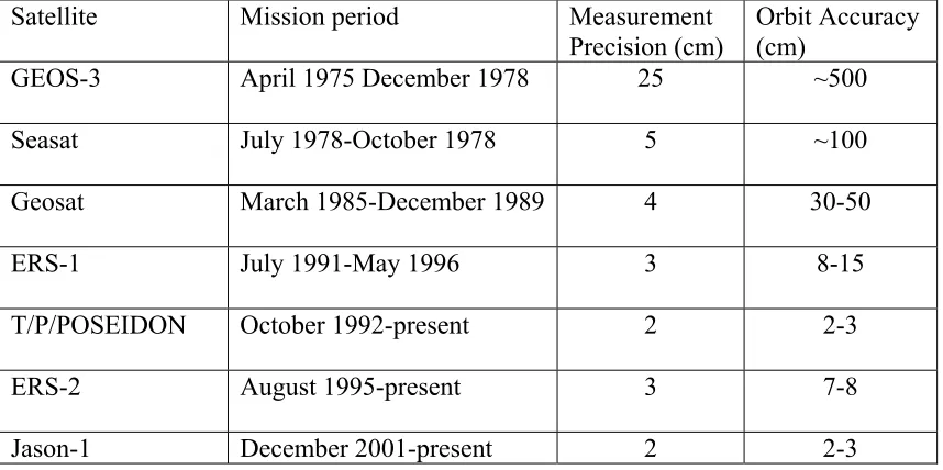
3.1 Summary of Satellite Altimeter Measurement 41
Precisions and orbit Accuracies
5 .1 Comparison of means wave height from MMS 76
and T/P for area A2, B3, C5, D6 and E7.
5.2 Comparison of marginal probability occurrence 79
of wave height between T/P and GWS
5.3 Weibull Parameters for Wave Height Exceedance 80
Cumulative Probabilities
5.4 Comparison of marginal probability occurrence of 82
wave height between T/P and PRSS
5.5 Comparison of marginal probability occurrence of 84 wave height from T/P data with NDBC buoys data.
5.6 PRSS Measured data 87
5.7 Davies Method 87
5.8 Gommenginger Method 88
5.9 Hwang Method 88
5.10 Comparison of marginal probability occurrence of 89
LIST OF FIGURES
FIGURE NO. TITLE PAGE
2.1 Joint probability distribution function diagram 16
(scatter diagram) for area 62, (BMT 1986)
2.2 A microwave Doppler radar looks at small patch of 26
the sea surface (Tucker, 1991).
2.3 A measured H.F radar backscatter spectrum 28
(Tucker, 1991)
2.4 How corner-cube reflection works for H.F. radar. 29
(Tucker, 1991)
2.5 The satellite borne precision altimeter used for 32
measuring wave height (Tucker, 1991)
2.6 SAR image of waves diffracting (Tucker, 1991) 33
2.7 GWS data area for Southeast and North Australian. 35
Sea (BMT, 1986)
3.1 Interaction of an altimeter radar pulse with a 39
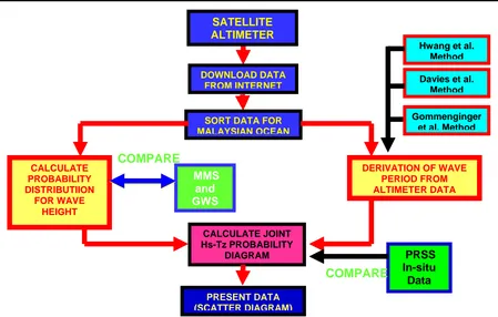
4.1 The flowchart of procedure to develop Malaysian 61 ocean wave database using satellite altimetry
4.2 TOPEX/Poseidon text data containing the date, 62
location, SWH and etc.
4.3 The 2º x 2º for latitude and longitude separation for 63
Malaysia ocean area.
4.4 Flow chart for the computer program 71
5.1 Location of selected area for comparison 74
5.2 Comparison of average wave height from MMS 76
and T/P for area A2.
5.3 Comparison of average wave height from MMS 77
and T/P for area B3.
5.4 Comparison of average wave height from MMS 77
and T/P for area C5.
5.5 Comparison of average wave height from MMS 78
and T/P for area D6.
5.6 Comparison of average wave height from MMS 78
and T/P for area E7.
5.7 Comparison of marginal probability of occurrence 79
of wave height between T/P and GWS
5.8 Probability distribution of wave exceedance 80
5.9 Comparison of marginal probability occurrence of 82
5.10 Location of selected buoy 42039 (black box area) 83
5.11 Comparison of marginal probability occurrence of 85
wave period from T/P data with NDBC buoy data
5.12 Comparison of marginal probability occurrence of 89
wave period between T/P, PRSS and GWS data for area
LIST OF ABBREVIATIONS AND SYMBOLS
BMT - British Maritime Technology
CEOS - Committee on Earth Observation Satellite
CNES - Centre Nationale d’Etudes Spatial
CODAR - Coastal Oceans Dynamics Application
ECMWF - European Centre for Medium Range Weather Forecasts
Envisat RA2 - Environmental Satellite Radar Altimetry 2
ERS - European Remote Sensing
ESA - European Space Agency
Geosat - Geodatic Satellite
GFO - Geosat Follow-on
GWS - Global Wave Statistic
H - Wave height
H.F. - High Frequency
Hs - Significant wave height
Hv - Visual wave height
JPL - Jet Propulsion Laboratory
JWA - Japan Weather Association
MGDR - Merged Geophysical Data Record (MGDR)
MMS - Malaysian Meteorological Services
NASA - National Aeronautic and Space Agency
NCEP - National Centers for Environmental Prediction
NDBC - National Data Buoy Centre
NESDIS - National Environmental Satellite, Data and Environment
Service
NOAA - National Oceanographic and Atmospheric Administration
ODAP - Oceanographic Data Acquisition Project
OSCR - Ocean Surface Current Radar
R - Range between satellite and ocean surface
R.M.S - Root Mean Square
S - Satellite orbit
SAR - Synthetic Aperture Radar
Seasat - Sea Satellite
SGOWM - Spectral Global Ocean Wave Model
SSH - Sea surface height
SWH - Significant wave height
T - Wave period
Tz - Zero-crossing wave period
T/P - TOPEX/Poseidon
U - Altimeter windspeed
WAM - Wave Model
WRB - Wave Rider Buoy
WWA - World Wave Atlas
η2 - Surface elevation
σs - Shape of return pulse
LIST OF APPENDICES
APPENDIX TITLE PAGES
A Advantages and disadvantages among the wave 104
measurement methods.
B Several methods for wave measurement 105
C Example of Monthly Summary of Marine 106
Meteorological observation, 1996 from MMS
CHAPTER 1
INTRODUCTION
1.1 Background
Ships are built for the purpose of carrying men, material or weapon upon the sea. In order to accomplish its mission, ship must posses several basic characteristics. It must float in a stable upright position, move with sufficient speed, be able to manoeuvre at sea and in restricted waters, and be strong enough to withstand the rigors of heavy weather and wave impact. To design a ship with these features, naval architects must have an understanding of ship dynamics.
With a simple knowledge of hydrostatics a naval architect can produce a ship that will float upright in calm waters. However, ships rarely sail in calm waters. Waves, which are the main source of ship motions in a seaway, affect the performance of a ship considerably and the success of a ship design depends ultimately on its performance in a seaway.
safety and survivability of the ship, increased demands on powering, or the severity of the motion-induced accelerations, which prevent the ship’s crew, equipment and systems from functioning effectively. More often then not, we end up with ships and boats that fail to perform in rough weather condition.
Since the end of the 1950’s new analytical methods were developed to predict the response from definition of the wetted surface of the hull and some simple
measure of mass distribution. Throughout this performance assessment process, a good and reliable wave data is required. For example, Hoffman and Fitzgerald (1978) emphasized the importance of the simulating operation of crane vessel in realistic waves. Their earlier work shown that errors up to 100% in magnitude of motion may occur arising from the use of inadequate wave data. Data is required regarding the probability of occurrence of wave heights and period in Malaysian waters. This data are presently available based on publications by periods in Marine Meteorology and Oceanography, Malaysian Meteorological Service, example MMS (1996). Also, sometimes data published by BMT (1986) is used. Although there is some problem in accuracy of data based on voluntary reporting, for time being we have to rely on these for probability of occurrence of wave heights and periods.
Since the available wave data for Malaysian ocean are not reliable and comprehensive, new effort to collect wave data must be made. Ocean wave
measurement from satellite combined with global wave and atmospheric numerical models are dramatically changing our way of obtaining ocean wave data for
engineering purposes. Satellite observations are now at the point of providing reliable global long-term wave statistics. Thus, the aim of this project is to develop Malaysian ocean wave database using satellite in the mission to provide the reliable wave data for Malaysia.
altimeter reflects from the wave crest, later from the wave troughs. The reflection stretches the altimeter pulse in time, and the stretching in measured to calculate wave height. The travel time of this pulse is then recorded. The significant wave height is derived from the stand up characteristic of a pulse waveform reflected from the sea surface, crests and troughs on that occasion. The wave data measured by one satellite called TOPEX/Poseidon is available free online given by Jet Propulsion Laboratory (JPL). By verifying the accuracy of the satellite altimeter data, continuous
measurement of the wave data of Malaysian ocean can be done at much effective and inexpensive way.
1.2 Objective of the Study
To derive Malaysian ocean waves data using satellite altimetry and present it in a form suitable for engineering purposes.
1.3 Scopes of the Study
This study involves the use of satellite data, processing it using certain techniques and presenting in formats useful for engineering purpose. The study is limited by the following boundaries:
i. The study will only involve TOPEX/Poseidon satellite.
ii. Only wave data from the satellite and relevant associated data will be
analysed.
iii. The case study will involve a portion of sea areas; however the method will
CHAPTER 2
LITERATURE REVIEW
2.1 Introduction
This chapter is giving an overview of the requirement of wave data, the wave data source and currently available wave data collection.
2.2 Wave in Marine Engineering
Knowledge of ocean waves is essential for any activity connected with the
seas.The largest forces on ships, as well as on offshore rigs and coastal defences,
To provide efficient advice for these activities not only significant wave height (SWH) but also measurements of the mean wave length and the mean wave direction are necessary. These integral wave parameters are available from a few stations and from ships measuring on opportunity. Certainly, more valuable is the knowledge of the entire wave spectrum, which describes the frequency-direction distribution of the wave energy density.
2.2.1 Coastal Engineering
Waves, generated primarily by the wind, propagate from the ocean to the shoreline across the continental shelves. These waves undergo many processes before they dissipate in the surf zone; refraction, diffraction, shoaling, and breaking. The energy and momentum associated with the waves arriving at the surf zone used to create longshore and cross-shore currents. Wave not only damage breakwaters, but also move the sand comprising beaches and deposit them somewhere else. Taken over long periods for this sand transported away from the site than toward it, this becomes the ‘long-shore drift’, which is an important geological phenomenon. Beside that waves can also be generated by submarine earth quake, volcanic eruption and tides.
other side of this coin, many researches are being conducted worldwide to develop predictive models of this erosion process.
Numerous devices have been devised to stop the erosion process. These can be divided into two basic types which is the hard and soft structures. Hard structures have been the traditional tool of the coastal engineers. These include groins
(structures oriented perpendicular to the shoreline to slow the transport of sand along a shoreline), jetties (placed at inlets to keep sand from the navigational channel), breakwaters (to reduce wave action in harbours), and sea walls (to prevent the erosion of the upland). The soft structures are those that are more natural. The
primary example is beach nourishment, which is the placement of sand on an eroding beach. Nourishment is a short-term measure, as it does not fix the cause of the
erosion; however, it is the only method that involves adding sand to the coastal system. Mangrove is also one of the natural coastal protections and believed to have reduced the damage caused by the recent Tsunami in December 2004.
2.2.2 Seakeeping
Seakeeping calculations are important in assessing the performance of a floating structure. It is particularly the operability aspect, and critical for small crafts such as patrol boats. Unlike most large ships, which use the oceans only as a
As the descriptive tool for seakeeping events, one way considered being the most useful for direct calculation of many valuable statistics is uses the energy spectrum. The pioneering work of Denis and Pierson (1953) on the application of superposition and spectral analysis techniques to seakeeping studies revolutionized seakeeping analytical studies. The energy spectrum is simply a presentation of the squared amplitudes of the frequency component of the sample records. This type of presentation, which indicates an estimate of the true spectrum, permits the treatment of ship behavior in the frequency domain so that ship performance can be related to the frequency response characteristics of the ship. Resultant responses of the ship can be estimated from the sum of responses of the ship to a train of individual regular waves of known frequencies (Omar Yaakob et al., 2003).
The wave incidents on the vessel are assumed to be long-crested. For such waves, the way in which the energy of the sea distributed at various encounter frequencies is given by the sea spectrum Sζ (ωe). By the principle of linear superposition, the sea spectrum can be related to the motion spectrum through the transfer function or response amplitude operator, RAO. If the motion RAO per unit wave amplitude or the transfer function at various encounter frequencies are
designated H (ωe), the spectral response of the selected response is Sr (ωe) then the particular seaway is given by:
Sr(ωe) = Sζ(ωe) x │H(ωe)│² (2.1)
The above method is normally used to predict motion responses of floating vessels. The sea spectra in this case are either actual sea-spectra measured at sea or idealized theoretical approximation such as Bretschneider, Pierson-Moskowitz or ITTC spectral formulations (Bhattacharya, 1978).
Equation (2.1) is also useful in full-scale experimental studies. If the time series of the waves heights incident on the vessel and the associated vessel motion response can be measured, Sζ(ωe), Sr(ωe) and hence H(ωe) can be calculated. This method is indeed useful, because it will enable us to derive the transfer function and hence RAO from the response spectrum of the vessel under test using
The transfer functions obtained in this manner can be used for comparison with RAOs from theoretical studies. Also, they can be used to estimating the response of the vessel in other seaways for which spectrum can be defined.
In absence of actual sea spectra, theoretical sea spectra are used. There are various theoretical representations of the sea spectra. Standard textbooks on waves mechanics or seakeeping refer to these spectra representation with various names such ITTC, ISSC, Breitschneider, Pierson-Moskowitz, and JONSWAP etc., see for example Bhattacharya (1978). Most of these belong to a general class of spectra referred to as the gamma-spectra. The gamma-spectrum has the standard form:
S(ω) = Dω-1 exp –Bω-n (2.3) The four parameters D, B, l and n control the shape of the spectra. The parameter l determines asymptotic behavior of the high frequency tail of the spectrum. Parameter
B is scale parameter of the frequency linked to the peak frequency, Ω through:
B = 1/n Ωn (2.4)
Parameter D determines the overall level of the spectral density and does thus indicate the general severity of the sea state. D is normally considered a universal
constant D=αg² where α is Philips constant equal to 0.0081. The frequently used
gamma spectrum is Pierson-Moskowitz spectrum. It has the form:
S(ω)=0.0081g²/ω5 exp -5/4(ω/Ω)-4 (2.5) i.e. the values of l and n are 5 and 4 respectively.
For not fully developed sea, the spectrum has distinct peaks and to take these into account, peak-enhanced Pierson-Moskowitz spectrum is proposed and renamed as JONSWAP spectrum:
S(ω)=0.0081g²/ω5 exp -5/4(ω/Ω)-4 +exp -1(ω-Ω)² /2(σω)² ln γ } (2.6) In this case γ is the peak enhancement factor, the effect of which is to increase the peak of the spectrum.
tailored to the local eave conditions should be used. Hoffman and Fitzgerald (1978) emphasized the importance of simulating the operation of crane vessel in realistic waves. Their earlier work has shown that errors up to 100% in magnitude of motion may occur arising from the use of inadequate wave data. Soares and Trovao (1992) investigated sensitivity of seakeeping prediction to spectral models and concluded that short-term responses are sensitive to the type of spectral model used while for long-term predictions only Pierson-Moskowitz model could be used.
Thus, it is important to have an accurate knowledge on the characteristics of the ocean waves when estimating the seakeeping performance of ships at sea (Ogawa et al., 1997). The wave used for the design ship is long-term data in all condition. Therefore, there is a need to establish the method of continuous wave data collection (Sakuno et al., 2003).
2.2.3 Offshore Engineering
Waves are generally the most important environmental factor producing forces on offshore structures. The design of offshore structures used for oil and gas present problems, due to environmental hazards from wind and current forces and the weight of the structure. In traditional design techniques the structure is first designed to withstand the most severe conditions which it is likely to meet in 50 or 100 years. Thus, as well as an estimate of extreme wave conditions; the statistics of all waves throughout the year have to be specified. The system for reliability techniques has been developed. In these, the probability distributions of the loads are calculated and compared with the ability of the structure to withstand these loads, also on a
In relation to the development of offshore oil and gas production at the offshore sea, there was a big push to gain enough knowledge to ensure the safety of the offshore structures in relation to the environmental forces. Oil price rises caused by high oil demand in the 1970s has prompted offshore development throughout the world in order to be self sufficient. However, there is plenty left to do as more sophisticated methods of design are introduced by engineers. An example is that designers now wish to take advantage of the low probability that the adverse extreme environmental factors will all occur simultaneously, but oceanographers cannot yet provide them with the necessary information on joint probabilities of occurrence (Tucker, 1991).
2.2.4 Wave Power
The power is very variable, of course, so that there must be alternative methods of generation available. This means that the cost of the power has to
compete with the cost of the fuel saved and not with the total generating costs. While solar radiation and winds are distributed over the planet’s entire surface, wave energy is concentrated along coastlines, which total about 336,000 km in length. At a global renewable rate of 1012 to 1013 watts, the average wave energy flux worldwide is of the order of several to a few tens of kilowatts per meter of shoreline (kW/m). Thus the energy density of ocean waves is at least an order of magnitude greater than the natural processes that generate them.
countries with only few ideals that show promises in its ability to capture and convert wave energy effectively. During 1970s, an increased interest on wave energy
conversion was seen due to the dramatic increase in oil prices especially in Europe. The greatest efforts were concentrated in United Kingdom, Norway and Japan. Efforts by others European nations and countries such as Sweden, Portugal, Denmark, India, China, Australia and United States also contributed to the advancement of wave energy conversion techniques and devices (Pin, 2005).
After a series of research into the possibilities, it soon became apparent that the available wave data were inadequate both to assess the resource and for design of the wave energy converters. Directional information is needed, and the techniques for routine directional measurement were only just being developed. It was therefore necessary to develop techniques to provide a long term measurement of the wave and this opportunity seen in the remote sensing technique. What the designers required was a set of directional wave spectra representative of the long-term wave climate, which they could use in model basins to test the overall performance of their devices. Some clever and ingenious devices to harness the power were designed and tested at model scales. In the end, none seemed capable of development into economic
systems where the competition was large mainland fossil-fuelled generating stations. However, where the competition is relatively small diesel generators, which is typical of the situation on islands, then the economics look more promising, and developments of this type are under way at the present time (Tucker, 1991).
2.3 Wave Data Sources
Based on the variety of the requirement for wave data, there are also various categories of wave data available such as instrumental measurement, visual
origin of data (see Appendix A). For example, whether the visual observation is the most useful data for wave data requirement, the probability of wave height of the ship report is thought to be smaller than other data sources because ships tend to try to avoid the storm seas. On the other hand, buoy measurement is considered to be one of the best sources of information since it measures wave mechanically, however it has a disadvantage of limited number of deployments for vast area of the oceans (Ogawa et al., 1997). Although there are many types of sensor working under remote sensing method and it seem all of them had accuracy and derivation algorithm problem, but the satellite altimeter data seems to be one of those fields where optimist feel that the promise is great. The information below briefly explain about this wave data available in sort of the principles and how its work.
2.3.1 Instrumentals Measurement
Wave instrumentals measurement or direct observation was the most accurate way to measure the wave height concerning the area of each particular study. But this method needs a highest cost, expose to the vandalism and unfortunately scarce
limitary point data in the fields of wide areas. For example, Draper et al. (1965, 1967, and 1970) presented statistics from measurements performed with a Tucker wavemeter at some Ocean Weather Stations (OWS), during a period of 3-4 years, but the total number of measurements of each station corresponds roughly to only one year of complete data. This is too short length of time to allow the statistical confidence necessary to long-term predictions (Gonzalez et al., 1991). Thus this measured wave data can only be used to calibrate the others measurement. There are four main categories of instruments to measuring the wave, which are known as wave staff, sub-surface sensor, buoys and shipborne systems (See Appendix B).
special structure. The output can be recorded on site, telemeter to shore, or sent along a cable. One problem, which is often quite serious, is that they need to be mounted well away from any sizeable structural members: 10 diameters away. The examples for this wave staffs are stepped-contact staffs, resistance-wire staffs, capacitance-wire gauges and the Baylor wave gauge.
Generally sub-surface sensors are mounted on or near the seabed and are either self-contained and therefore have to be recovered and replaced at regular intervals, or connected to shore via a cable. A snag with the former is that a malfunction may result in a considerable length of data being lost before it is
downloaded. In the case of the latter, the cable route must avoid areas where trawlers operate or ships anchor. The examples for this measuring system are pressure
sensors, inverted echo sounders and particle velocity meters.
Apart from remote sensing devices, the only way of satisfying this
requirement is to use sensors, which are in buoy or small vessels. There are many offshore buoys deployed in the oceans mainly by meteorological agencies, and it has been found that a wave-recording buoy can gives results, which are not influenced by proximity of a structure. They are considered to be unbiased and the most reliable gathering wave information since they measure waves by mechanical or electronic instruments. Despite with these advantages, the buoy has a reduced area of coverage and the limited availability, which is often due to commercial restrictions (Gonzalez et al., 1991).
A small buoy floating on the sea surface moves up and down with the waves. Its vertical acceleration can be measured, this can be integrated twice to give the vertical displacement. Although the concept is simple, there are a number of
A number of devices have been devised which rely on the attenuation of waves with depth, in effect using the deep still water as a reference. Although some of these have been used successfully for short periods, they have largely fallen into disuse following the successful development of accelerometer buoys. Most buoys telemeter the wave data to a platform or to a shore station, though some also record on board to improve the data return for historical data. Direct radio telemeters can be used for short range. For longer ranges, buoys have been designed which telemeter via satellites. In this case some data compression is required to reduce the number of bits to the capacity of the satellite channel. Gonzalez et al. (1991) describes a system in which a Wave Buoy transmits by radio to a nearby ‘mother’ buoy that is enough to contain adequate battery supplies and which is retransmits the data via
GEO/METEOSAT satellite. This has a larger data capacity. The examples for buoys are Pitch-roll-heave buoys, ‘Clover-leaf’ buoys and Particle-following buoys.
The Shipborne Wave Recorder (SBWR) was the first device capable of recording waves on the deep sea during a storm. Although not very accurate by modern standards, its cheapness to run and high data return have led to its extensive use. Mounted symmetrically on each side of whether ship and light vessels. Each contains a vertical accelerometer mounted on a critically damped short period pendulum, and a pressure sensor connected to the sea through a hole in the side of the ship. The accelerometer outputs are integrated twice and added to pressure signals, giving in each case the surface elevation relative to a fixed horizontal plane. These concepts are very simplified of what actually happens in practice. The
2.3.2 Visual Observations
There is a huge volume of observations of waves from ships in normal service all over the world, and these are held in data banks of various meteorological offices. A major source of visual wave data is the compilation made by Hogben and Lumb (1967), which cover most of the ship routes to and from Europe. The Pacific Ocean is not so well documented but this can be supplemented with the data from Yamanouchi and Ogawa (1970), which covers that ocean in detail. Another important compilation is due to Walden (1964), containing visual observations performed in the North Atlantic Ocean Weather Stations (OWS), during a period of 10 years.
As the wave statistical data, generally, are often shown in the form of occurrence frequency diagram, correlation table, of significant wave height and average wave period. However, Global Wave Statistics atlas, Hogben et al. (1986) (GWS) (see Figure 2.1) wave data presented in terms of joint probability distribution of significant wave heights and zero-crossing wave period for the global selection of 104 sea areas. The data represent an updated and corrected version of the Hogben and Lumb (1967) data. The observations are divided into subsets for each
Figure 2.1: Joint probability distribution function diagram (scatter diagram) for area 62, (BMT 1986)
The format of its standard scatter diagram is derived by a rounded number of one thousandth (1/1000) for its print out version and accuracy of 0.000001/1000 for its PC version. The wind observations were used to improve the reliability of the wave statistics. Unfortunately, many of the voluntary observing ships do not have anemometer installed but determine the wind speed via visual estimation by relating simultaneous visual estimates of wind strength on the Beaufort scale, wave height and wave direction. These are analysed on both a seasonal and an annual basis (Tilo and Stephan, 2000).
There are the advantages and disadvantages on the visual observation method to derived wave data. According to Soares (1986), it has three important properties of wave data from voluntary observation ships that make it unique. The first and
probably most important aspect is that it already incorporates the effects of bad weather avoidance. By avoiding the very large storms due to early meteorological information the probability of failure of ship structures are from high sea states can be much reduced. Because avoidance measures are the result of subjective
the use of data from voluntary observation ship appears as the possibility of representing the effect and this makes the data of voluntary observing ships preferable for the analysis of ship structures. However it is inappropriate to the analysis of fixed structures such as platforms. In this case the data from the Ocean Weather Stations is more appropriate. Another advantage of the data from transiting ships is that it is collected along trade routes used by merchant ships, where the need for information is greatest. A third advantage is that the estimates of mean values are likely to have no bias. Because the observations are made in many different ship types and sizes, they show reasons supports the hypothesis of systematic differences between measurements made in different geographical areas. Although the
assessment properties of the sea states by visual observations involves a significant degree of estimation variability, but it is possible to collect large samples of data, which may compensate for the variability because it is relatively inexpensive procedure.
On the other hand, because of the visual data usually come from ship reports which is an important part of them are concentrating on the main shipping routs, these data bring up some shortcomings due to observation itself. Firstly, the wave height was reported in adverse climatic conditions tend to be overestimated by the observer and secondly, more ships sail in good weather conditions consequently samples are biased toward lower wave height values. The result is that this sample does not fit accurately of the lognormal model, which is usually appropriate for wave study, when the observations reported as calms are included in the sample (Gonzalez et al., 1991).
The visual observation also shows a large correlation coefficient and
tend to underestimate wave height from weather ship. Firstly, it was the larger size of the voluntary ships which would lead the observers to make the lower estimates. Secondly, voluntary ships can dodge some of the rough while the weather ships are always on station.
Not surprisingly, discrepancy between the Global Wave Statistics (GWS) and instrumental data is observed. For the considered locations, the GWS data both underestimate as well as overestimate significant wave height while the zero-crossing wave period (Tz) mean value is systematically overestimated for low Hs while it is underestimated for large Hs. The opposite effect is observed for the standard deviation of Tz. The marginal empirical cumulative distributions of Tz, indicate also that the GWS data may underestimate the extreme wave periods. However, the instrumental database applied in the study is too limited to draw general conclusion as well as to specify a regression of the instrumental data on the GWS data. The GWS data represent the average conditions for each of the 104 ocean zones, while the instrumental data used in the analysis are representative for specific locations only (Bitner-Gregersen and Cramer, 1994).
Some of the research had also shown that the GWS have a different quality at the different ocean areas. For example, Chen & Thayamballi (1991) had compared the effect of use of the GWS data contra hindcast data in ship response analysis. For some ocean zones the GWS data have led to higher responses and slightly higher fatigue damage. However, that was not the case for other ocean zones. Therefore it was concluded that two sets of wave data were not quite consistent and should be used with care. It is also show by Bitner-Gregersen et al. (1993), which had
compared the GWS data with the Wave Rider Bouy (WRB) and Oceanographic Data Acquisition Project (ODAP) buoy wave data, which was accepted as the standard wave measurements for design work at sea. The 20 years extreme values were evaluated based on the GWS data deviated from extremes obtained by use of the instrumental wave buoy data. It was indicated that the GWS data might
wave height. It was also indicated that the uncertainty involved in use of the GWS data contra the instrumental data might be larger than the variation in wave induced loads and fatigue damage, between the different ocean areas (Bitner-Gregersen and Cramer, 1994).
The bias of wave period mean value and standard deviation in GWS is smaller for the North Atlantic than for the other locations considered. Comparison of the GWS and instrumental empirical probability densities of Hs and Tz, presented by Andrews et al. (1983), confirms also that accuracy of the North Atlantic GWS data seems to be satisfactory. The North Atlantic area has a high density of traffic, resulting in a larger database for this area, and a better agreement with the instrumental data for this area is therefore also to be expected.
While the quality of individual observations is questionable and the other type of wave data is now available, visual observations of wave height are still the main source of statistical information of waves during the last twenty years, that covers most of the oceans areas for the prediction of extreme wave conditions to be used in the design of ship structures. Generally, when using ship observation, data have to be carefully checked and evaluated (Tilo and Stephan, 2000). The usefulness of these visual observations depends, however, on a proper calibration with the accurate measurements of the wave characteristics. For example, Hogben et al. (1986) compared the GWS marginal distributions for wave height and periods, for which statistics was given, corresponded to be necessary to apply any correction factors, usually used for estimating significant wave heights from visual wave height observations. From the different regression equations available, the one have been recommended by the International Ship Structures Congress are the ones due to Hogben and Lumb (1967):
Hs = 2.55 + 0.66 Hv (2.7)
height. It is not too large, being of the same order of magnitude of other uncertainty sources in the calculations of wave loads. However, accuracy of the data is still questioned in the literature (Gonzalez et al., 1991)
2.3.3 Wave Hindcasting
Hindcast wave data could be an alternative to visual wave observation. Compared with data from instrumental measurements, hincast data cover a much wider sea area and do not miss storms because of instrument malfunction. Hindcast techniques use records of wind speed to estimate corresponding wave conditions. This is achieved by modeling the process of generation and propagation of waves by wind (Gonzalez et al., 1991). The hindcast data as a good means of interpolating wave statistics between instrumental sites, they give data over longer periods and also give directional information, which is available from very few instrumental sites. The models described here are basically for deep water of intermediate depths. The final run-up to the coast or over shallow banks is a complicated matter.
This method has been carried out for many years, but the modern
development was triggered by Second World War, when in all theatres of war the Allies had to make landings on enemyheld beaches. An ability to predict the wave conditions was vital. Early methods were largely concerned with predicting the wave height and period from the local wind, taking account of the distance over which the wind was blowing its ‘fetch’ and the time for which the wind had been blowing at a more-or-less constant speed its ‘duration’. Such methods are still useful in certain circumstances. As the speed and capacity of computers develop, it became
The second generation of finite-difference model resulted from a clearer understanding of the energy transfer processes, in particular the third-order
processes, but had to simplify the representation of these because of the limitations of computer power at that time. Second-generation models have been in routine use for many years and large data sets have been built up. What usually stored is
sometimes known as ‘nowcast’ data: that is, the estimate of the wave field at the time of calculation taking into account the most recently available wind data. A preferred method to gain long-term wave statistics is to run wave forecasting models on historic wind data a process known as ‘hindcasting’. The historical wind information is more reliable then the real-time estimates of wind fields, partly because a
considerable quantity of late information can be incorporated. In hindcast model, it is usual to run the model for most severe to run it for a long continuous period (Tucker, 1991).
Increases in computer power and improvements to the algorithms for computing third-order wave-wave interactions have made it possible to develop a ‘third generation’ model in which the spectrum is developed step-by-step, using the full energy balance equation. Develop in recent year, the hindcasting are prepared using numerical wave models with the hindcast wind as input and using the physics of wave growth, transmission and decay (Carter et al., 1989). This has the advantage of not having to make priori assumptions about the spectral shape, and should therefore give better results in complicated conditions such as hurricanes.
Recently, wave data collection using hindcast method was generated by Japan Weather Association for global wave database. The database is the simulated wave data (wave height, wave period, wave direction and wind velocity) using JWA3G model, 1985-1999 (15 years). Time and grid intervals are 6 hours and 2.5 degree (about 250 km mesh) (Tilo and Stephan, 2000). Also, there is a Wave Model (WAM) [WAMDI Group (1988)], which was operated routinely at the European Centre for Medium-range Weather Forecasts (ECMWF) (Staabs and Bauer, 1998). Modelled Hs are provided from WAM (cycle 4) with global 3º x 3º grid and with forcing by
ECMWF 6-hourly wind fields. The modelled Hs fields are stored every 6 hours. The major improvement of WAM cycle 4 with respect to WAM cycle 3 is the dynamic coupling between the wave-induced stress and the atmospheric stress (Komen et al., 1994).
However, substantial uncertainty can be obtained from calibrations of hindcast methods. On the other hand, the hindcasting methods are not very accurate and considerably improved if the models are initiated and updated with others sources observations of wave height and period (Carter et al., 1989). In the last decade, the performance of wave models has significantly improved, due to improved accuracy in the wind forcing fields, and to the assimilation of altimeter data (total energy of waves). It has been shown that the assimilation of altimeter data in wave model improves the forecast of the Hs (Lefevere et al., 2003). For example, errors in wave modeling using WAM are caused mainly by incorrect wind forcing and less by insufficient resolutions. Since August 16, 1993, Hs from the European Remote Sensing (ERS) altimeter have been assimilated into the WAM model at ECMWF (Staabs and Bauer, 1998).
these major hindcast programs concern ocean areas which are already reasonably well documented by various types of wave data. Therefore they do not fill the gaps of the visual wave data and cannot be considered yet as a real alternative (Soares , 1986).
2.3.4 Remote Sensing in Wave
Remote sensing is one of the indirect observations and it is defined as making measurement by using electromagnetic waves, so that no mechanical disturbance of the sea-surface is caused. This indirect observation is not so sensitive comparing with the direct observation but we can get the data easily and cheaply in wide areas with the same instrument in short time of period. Remote sensing is widely applied to research of the ocean. At present the space-borne radars allow us to realize a global overview of the state upper layer of the ocean surface and to obtain information on its characteristics, such as significant wave height (altimeter), and wind speed (altimeter and scatterometer). This information is necessary for the solution of a broad list of problem in oceanology, meteorology, navigation and ocean safety engineering. Electronic wave scattered by the ocean surface contain the information on its characteristics. A wide range of electromagnetic wavelengths has been
successfully used, from infrared pulsed lasers to high frequency (H.F) radio waves travelling horizontally over the sea surface and being reflected back by sea waves of half their wavelength.
interpretation. Large amounts of effort have been put in these systems, but they are still not very accurate quantitative tools. The example of this type sensor is Synthetic Aperture Radar (SAR), H.F radar and Plan Position Indicator (P.P.I) ground based radar. There are various type of radar based on the position of the sensors transmit the electromagnetic such as Ground-based Radars, Airborne sensors and Satellite-borne sensors.
2.3.4.1 Ground-based Radars
a) Vertical Radar
b) Plan Position Indicator (P.P.I) Radar
P.P.I. radar is also ground base radar. Conventional high-resolution short-range ships radars are suitable for this application, with minor modifications. One complete sweep of the radar is photographed at suitable intervals. The gain is set so that the ‘sea clutter’, that is, the echoes from the sea-surface, is clearly visible. The height of the radar is fairly critical. As the height is raised, so the reflection of signals from distant waves increases, but at too great height the contrast is lost and the image of
the wave disappears. A height giving a grazing angle of about 0.5o at extreme range
seems to be about right. The precise physical mechanism at work in producing the backscatter pattern are not too clear, though in some cases it seems likely that reflections from the crest are being seen with the wave trough being shadow. Such installations are comparatively cheap and simple. They give the predominant direction of the waves, and this is very useful, in conjunction with a point wave recorder, for coastal engineering problems. Working further offshore in a depth sufficiently great so that changes in the phase velocity of the waves are negligible over the area of a radar image, navigation radar mounted on a ship or other suitable platform can be used with a more sophisticated system of analysis.
c) Microwave Doppler Radar
The third type of the ground base based radar is the Microwave Doppler radar. In concept, these shine a narrow microwave beam to illuminate a small patch of the sea surface, and measure the Doppler shift of the echo due to the very short Bragg-resonant waves being carried back and forth by the surface particle velocity due to the longer waves. If the wave system is considered as the linear superposition of many components, then for each component (in deep water) the particles travel in circular orbits. If all the wave components were travelling towards the radar, then the statistics of the particle velocities seen by the radar would be the same as the
statistics of the vertical velocities. When integrated, they would then give a
displacement time-history whose spectrum and statistics would be the same as those of a vertical displacement record. Note that this is not true when wave are nonlinear, so such radars cannot be used to measure the shape of extreme waves. However, they do measure the horizontal component of surface particle velocity correctly in
nonlinear waves, and this is a very useful measurement.
d) High Frequency (H.F) Radar
The H.F radar is now established as a powerful tool for measuring the patte of surface currents over an area out to a range about 30 km, with an accuracy of about ± 3 cm/s in all conditions. Much has been claimed for its potential for measuring directional wave spectra out to ranges of perhaps 150 km, but development of this still had a rather limited success. Three main practic
rn
the al versions f H.F. radar have been developed. The first was the CODAR (coastal oceans ynamics applications radar) intended for measuring both waves and current, and develop
tch ,
and one negatively Doppler shifted from the transmitter frequency. These lines
corresponded to echoes from the Bragg resonant waves travelling towards and away from radar. With no current, the Doppler shifts are equal to the frequency of the Bragg resonant wave, and therefore in the range 0.1 to 0.6 Hz approximately. If a component of the surface current is following towards the radar, it will increase the Doppler shift of the approaching wave and decrease that of the receding wave. o
d
by Barrick and Lipa (1979). The second was the Ocean Surface Current Radar (OSCR) developed by King et al. (1984) specifically for current measurement. The third is longer wavelength H.F. radar developed at the University of
Birmingham by Shearman et al., (1987) mainly for wave measurement.
Figure 2.3 : A measured H.F radar backscatter spectrum (Tucker, 1991).
For wave measurement, more complex second-order mechanism of
backscatter is therefore used. Hasselman (1971) and Barrick (1972) established this technique as the foundation. Because the hydrodynamic equations are nonlinear, two wave trains of different frequency and direction interact to form two further
The second mechanism works rather like a corner-cube reflector (See Figure 2.4). If two sea wave trains of suitable wavelengths are travelling at right angles to one another, then the radar waves can be reflected first from one and then from the other back to the receiver. In each case the Bragg resonant condition must be met at the angle of incidence, which will in general be different for each of the two wave trains. Thus, again, a signal will be received which covers a spectrum of Doppler
frequencies. The process is most effective when the two waves are travelling at 45o
to the axis of radar beam, giving another peak at a frequency of 23/4 fB. Other small
peaks can sometimes be seen corresponding to the third and fourth harmonics, but these are not considered in the analysis.
2.3.4.2Airborne Sensor
a) Radar Altimeter
Many attempts have been made to measure waves by using a narrow-beam vertical radar altimeter mounted in an aircraft flying low over the sea, so that the illuminated patch is small compared to the sea wavelengths of interest. These have
instrumental difficulties, partly to the cost and ther problems of flying aircraft, both during development and operationally, but
ore fundamentally because of the difficultly of interpreting the resulting records. The air
le to
cross the track of the aircraft and in sections of 1024 cells along the track. The resolution is 1.4o across the track and 1o along the track, with 15cm in surface elevation. The aircraft was flown at heights of
m across the track and about 5
along the track. The system is corrected for the roll of the aircraft, and for the oppler shifts in the wave spectrum due to the drift and forward speed of the aircraft. Ambig
s all been unsuccessful partly owing to
o m
craft is flying faster than the phase velocity of the waves, but there will be some component wavelengths and directions for which the resulting frequency as seen by the aircraft is near zero, and such waves are not measured. It is impossib keep an aircraft at exactly constant altitude, so that low-frequency noise is also introduced. In practice, this noise has seriously contaminated the results, even when a vertical accelerometer was used to measure the vertical motion of the aircraft and to compensate for it.
b) Surface Countering Radar
Walsh et al. (1985) describe an airborne surface contouring radar which measures the directional spectrum of the waves. This is across-track scanning radar, which contours the sea-surface in 51 cells a
200 and 400 m, giving surface resolution of 3 to 5 m
m D
of this system with other surface sensors gave very encouraging results. The system seems more suited to one-off experiments than for routine measurements, no
because of the costs of flying an aircraft routinely, but also because it seems un that the aircraft could fly at the low altitude required in the extreme conditions when routine measurements are most important.
c) Radar Ocean Wave Spectrometer (ROWS)
t only likely
his concept has been implemented from aircraft, but is in principle suitable r satellites. The short-pulse radar is directed at the sea surface at a relatively steep m the vertical for the proposed satellite instrument). The pulse is backscattered from the sea surface, and the time history of the
backscattered energy is analysed. The pulse is short enough to resolve the sea n the range direction, but the width of the illuminated patch several wavelengths, thus averaging wave travelling across the range direction and iving directionality. The returns from successive pulses are averaged in range bins fixed re
sure the shape of the Earth’s surface, and this has shown ome fascinating results. The microwave radar altimeter is conceptually the simplest f the active remote sensing instruments, and, after nearly two decades of spaceborne
T fo
angle of incidence (10o to 13o fro
wavelengths of interest i is
g
lative to the sea surface. The aerial is rotated to look at the sea successively in all directions. It is assumed that the law relating the backscattering cross-section σ0 to
the wave characteristics is known, so that the Fourier transform from each directional look can be related to the directional spectrum in a known way (Tucker, 1991).
2.3.4.3Satellite Borne Sensors
a) Radar Altimeter
A number of altimeters of the same general type have been flown. Their main application has been to mea
operation, it has become a well-developed and documented tool. The primary
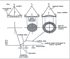
purpose for the development of the spaceborne altimetry was oceanic physics, where altimeters were proposed for the measurement of mean sea level and sea state. In addition to oceanographic applications, the satellite altimeter has proven to be a useful tool for studying the continental ice sheet of Greenland and Antarctica. The satellite altimeter is a nadir-pointing instrument designed to measure the precise time it takes a radiated pulse to travel to the surface and back again. If the orbital position of the satellite is known relative to a reference surface, then the measured time converted to range can be used to derive the elevation of the reflecting surface (See Figure 2.5) (Davis, 1992).
Figure 2.5: The satellite borne precision altimeter used for measuring wave height (Tucker, 1991).
b) Synthetic Aperture Radar
he Synthetic Aperture Radar (SAR) produces an image of the sea surface
(See Figure 2.6) the
T
image. However, the SAR image spectrum has turned out to be far from the actual wave spectrum and rather complicated post-processing is necessary for extracting quantitative wave information. The core of the methodology is Hasselmann’s non-linear ocean-SAR spectral transform develop in the early nineties. Despite intensive research over several years, there is still quite some way to go before the SAR-ocean
rsi ned from the
altimeter.
inve on reaches the accuracy for the significant wave height obtai
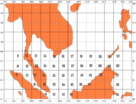
2.4 Currently Available Wave Data Collection in Malaysia
Presently, sources for wave data especially on wave height and wave period available in Malaysia for engineering purposes are limited. Researchers ha
on the visual observation data and the wave spectrum, which are based on we sea conditions and parameters for engineer
ve to rely stern ing applications. A brief information and ummary on the status of available wave data collection in Malaysia is presented here.
ritish Maritime Technology (BMT) provides the data that contains statistics of ocean wave climate for whole globe generally known as Global Wave Statistics atlas, Hogben et al. (1986). The data are presented in terms of probability
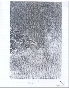
distributions of wave heights, periods and directions for global selection of sea areas. The data have been derived by a quality enhancing analysis of a massive number of visual observations of both waves and winds reported from ships in normal service all over the world, using computer program called NMIMET (Tucker, 1991). However, there are disadvantages on this data, which is based on visual observation from ship. As ships will try to avoid stormy areas, fewer reports are available from stormy area. Secondly, the whole of South China Sea, Straits of Malacca and the G
inaccurate data for particular area. And thirdly, there is no data for certain critical areas for example Indonesian, Southern Philippines and North Australian sea areas (See Fi
ccuracy is s
B
ulf of Siam are lumped into one area, which is area 62, and hence this will provide
gure 2.7).
questionable. Also, it is based on voluntary reporting and thus, no data were available for some areas.
6).
isadvantage on these two devices. For example, the buoy was located in the atoll structure in Layang-layang region at Sabah. The waves thus measured are near th
al range data
eld.
ave Figure 2.7: GWS data area for Southeast and North Australian Sea (BMT, 198
MMS also provides the forecasting wave data and buoy data but there are advantage and d
e atoll instead of the open sea. This in-situ reference also suffers from the relatively small number of data sets and the incomplete coverage of the natur of variations of Hs. MMS also uses a wave-forecasting model called WAM. The provided by the MMS is presented on monthly charts with individual values in
squares of 2o latitude by 2o longitude and with forcing by MMS 6-hourly wind fi
Errors in wave modeling using WAM are caused mainly by incorrect wind forcing and less by insufficient resolutions (Staabs and Bauer, 1998).
database collected by Petronas Carigali Sdn. Bhd. But these wave data are not published and not easily available to the public.
2.5 Summary
Early in this chapter, the importance of the wave data to the marine
engineering field, especially seakeeping is briefly described. It is clear that in order to obtain a good and reliable wave data, the raw data collected must be subjected to the precise calculation. A reliable and efficient device will need to be deployed
besides the strong and stables s waves. This was
followed by reviewing the various methods of measurement, observation and
forecasting to get the wave data. The advantages and disadvantages of these methods are com ared
two sources of published data for wave are publicly available in Malaysia; which is Global Wave Statistics (GWS) from British Maritime
Technology Ltd., (1986) and the Monthly Summary of Marine Meteorological Observ
g to rely on
and for others requirement are not reliable and insufficient, new effort to collect wave data must be made. One method which is
bservation and collection of wave data via remote sensing seem to have great otential for development. The next chapter will describe the satellite altimetry
chnique in detail.
tructure to withstand the severe
p
Presently, only
ations from Malaysian Meteorological Service (MMS). These data were based on the visual observations covering selected areas mainly along shippin routes. Marine technologists have no viable alternatives and therefore have these for the time being. Since the available wave data for engineering design calculations for Malaysian ocean
CHAPTER 3
SATELLITE ALTIMETRY
3.1 Introduction
The previous chapter has shown that wave data is an important input to engineering design calculations. A number of sources of wave data and their respect
ter ive strengthen and weaknesses have been reviewed. One important
development in this field is satellite altimetry. This chapter introduces concept and application of satellite altimetry.
3.2 Past and Present Satellite Altimeter
The ‘proof of concept’ of a satellite radar altimeter was established by an instrument carried on SKYLAB in 1973. The United States satellite SEASAT, which was only operational for three months in 1978, was the first satellite with an altime
to give global coverage, from 72oS to 72oN. An earlier satellite of NASA, GEOS-3
it did not provide global coverage. It was not until March 1985 that another altimeter was launched, in the US Navy’s satellite GEOSAT. As indicated by its name
(GEOdetic SATellite), the satellite’s primary purpose was to measure the marine geoid with high precision. Because of the strategic value of the gravity field which is obtainable from the geoid, the data from the first 18 months of observations we classified b
re ut some data including wave height values have been released. The classified geodetic mission ended in September 1986, and during October the satellite s orbit was altered, placing it into a 17-day repeat pattern in which it operated until the satellite failed in January 1990; although there was a significant decline in data coverage from about March 1989. Thus GFO has provided, for the e of wave data (from 72oS to 72oN) (Carter et al., 1989).
fe. arth
radar
t for studying variability of sea level and associated global climate changes, but also provides excellent estimates of
SWH but only from 66oS to 66oN (Carter et al., 1989). The main instrument is the
dual fre e
vy’s
-’
first time, several years of near-global coverag
Then, the European Space Agency’s ERS-1 was launched in July 1991 into an orbit covering 82oS to 82oN, and is still working well, long after its planned li The satellite ERS-1 was designed to carry out a wide ranging programme of E remote sensing research. To achieve this, ERS-1 operates a suite of remote sensing instruments, including a radiometer, scatterometer, synthetic aperture radar and altimeter. It has operated in various repeat-orbits: 3-day, 35-day and currently 168-days. Its replacement ERS-2 was launched in March 1995; but ERS-1 also continue. The US/French satellite T/P was launched in September 1992 into a 10 day repeat orbit. Its primary task is monitoring sea surface heigh
1, in December 2001, and ENVISAT, in April 2002, five altimeters are flying together.
3.3 Altimeter Principles and Techniques
The satellite altimeter is nadir-pointing instrument designed to measure the precise time it takes a radiated pulse to travel to the surface and back again. If the orbital position of the satellite is known relative to a reference surface, then the measured time, converted to range, can be used to derive the elevation of the reflecting surface. A very narrow pulse (<10 ns) is transmitted in order to obtain a small range resolution. In addition to measuring range, the altimeter records an averaged number of return echoes (typically 100), and estimates other geophysical parameters such as ocean wave height and return pulse magnitude. A diagram altimeter pulse interaction with a flat surface and the corresponding return echo is shown
As the incident pulse strikes the surface, it illuminates a circular region that
increas of
will
f the of the
in Figure 3.1, reproduced from Davis (1992).