Multidimensional analysis of time-resolved charged
particle imaging experiments
Vincent Loriot1,2,3ID, Luis Bañares1∗ ID and Rebeca de Nalda2ID
1 Departamento de Química Física (Unidad Asociada I+D+i al CSIC), Facultad de Ciencias Químicas,
Universidad Complutense de Madrid, 28040 Madrid, Spain
2 Instituto de Química Física Rocasolano, CSIC, C/Serrano 119,28006 Madrid, Spain
3 Institut lumière matière, UMR5306 Université Lyon 1-CNRS, Université de Lyon 69622 Villeurbanne cedex,
France
1
2
3
4
5
6
7
8
9
10
11
* Correspondence:[email protected]
Abstract:Wepresentatutorialtorealizeamultidimensionalfittingprocedurecapableofextracting
alltherelevantinformationcontainedinasequenceofchargedparticleimagesacquiredasafunction
oftimeinfemtosecondpump-probeexperiments. Theimagesarereproducedusinga3Dfitting
method,whichprovidesthevelocity(orcenter-of-masskineticenergy)andangulardistributions
containedintheimagesandtheirtimeevolution.Adetailedexampleofthemethodisshownthrough
theanalysisofthetime-resolvedpredissociationdynamicsofCH3IontheB-bandorigin[Gitzinger
etal.,J.Chem.Phys.133,234313(2010)].Weshowthatthemultidimensionalapproachisessential
fortheanalysisofcompleximagesthatcontainseveraloverlappingcontributionswherereduced
dimensionalityanalysescannotprovideareliabledescriptionofthefeaturespresentintheimage
sequence.Thismethodologycanbegeneralizedtomanytypesofmultidimensionaldataanalysis.
Keywords:Femtochemistry;VMI(velocitymapimaging);Multidimensionalanalysis.
PACS:07.05.Kf,33.80.Gj,07.77.Ka 12
A broad range of experimental scientific fields have moved over the last few years from the study 13
of scalar or vectorial quantities (i.e.measurement of a magnitude or a string of data as a function of a
14
relevant variable) to the acquisition of images (i.e.2D sets of data). The broad availability of cheap
15
charge-coupled devices (CCD), the larger storage capabilities and the faster communication protocols 16
have contributed to this remarkable change. In particular, in the field of Atomic and Molecular 17
Physics, traditional methods, such as time-of-flight detection of ions or photoelectrons, are increasingly 18
being replaced by techniques like ion or photoelectron imaging, or even ion-photoelectron coincidence 19
imaging, for the study of photoionization, photodissociation, reaction dynamics or molecular alignment 20
[1–8]. The acquisition of spatially-resolved data on the final position of these particles can yield a 21
wealth of information of the process under study that was unimaginable with previous methods. In 22
the analysis of these data it has been common practice to analyze either integrated sections or cuts of 23
the images to obtain 1D information that is then analyzed with standard 0D or 1D fitting procedures 24
[9–12]. In many cases, the richness of the information that can be extracted from the data is lost. 25
Multidimensional analysis can separate certain contributions that are often the key to unravel the 26
dynamical processes. 27
In this work, we present a multidimensional fitting solution dedicated to obtain the best fit to 28
the complete set of data contained in a time sequence of a sequence of velocity map images measured 29
in femtosecond pump-probe experiments, through parameterized functionals that describe radial 30
and angular properties of the particle distribution as a function of time. As will be shown, the 31
multidimensional fit becomes essential for instance when contributions with different time behavior 32
are overlapping. Additionally, for those cases where the initial guesses for the parameters or functional 33
forms of the fit are misguided (on the number or nature of the contributions to the image, on the 34
time behavior of anisotropy, etc. . . ), discrepancies can be detected easily through the use of the 35
analysis of the residuals. It is important to note that the multidimensional nature of the fit allows the 36
discrimination of the different contributions to the images, in a manner that a reduced-dimensionality 37
analysis cannot achieve. This method has revealed its value in a number of contributions where 38
the need for discrimination of overlapping contributions in charged particle images was crucial 39
[13–18]. The method is analogous to the global 2D fit approach used in Stolow’s group [19–22] but 40
can easily be extended to extra dimensions such as the anisotropy, the temperature, the intensity 41
dependence, measurements in coincidence, etc. . . With some modifications, the method can be equally 42
applied to other problems, such as the detection of spectrally and spatially resolved X-rays from 43
high-harmonic generation [23], or temporal-spectral-spatial ultrashort pulse characterization [24–26] 44
and time-resolved time-of-flight measurements [27]. For each particular application, functional shapes 45
and dependences have to be adapted, but the strategy presented here is of general applicability to the 46
study of 2D or higher dimensionality data. We describe the procedure in a pedagogical way to adapt 47
any algorithms of optimization to a multidimensional analysis. 48
The paper is organized as follows. In Sec.1, the method to construct velocity map images and to
49
describe their time evolution is presented, including both 3D and 2D versions. The multidimensional 50
numerical fitting procedure is explained in Sec. 2, and Sec. 3is dedicated to the application of the
51
method to a case example: the femtosecond pump-probe velocity map imaging (VMI) experiment on 52
CH3I predissociation on theB-band. Sec.4closes the paper with the main conclusions.
53
1. Construction of a sequence of velocity map images and description of its time evolution 54
The first demonstration of charged-particle imaging applied to reaction dynamics was made by 55
Chandler and Houston. In their 1987 work [1], they showed how it is possible to record, at once, the 56
entire spatial distribution of fragments originating from a photodissociation event. In this way, within 57
the resolution limits, it is possible to directly measure the angular and velocity distributions of the 58
products of a chemical reaction. The technique of ion/photoelectron imaging made a giant leap a 59
decade later with the discovery by Eppink and Parker of the technique that is known as velocity map 60
imaging [2], where through the use of open-lens electrodes with appropriate voltages, it is possible to 61
work in a configuration where products of a photodissociation event with the same initial velocity 62
vector are imaged onto the same position in the detector. This implies that the observed images are 63
in fact 2D projections onto the plane of the detector of a velocity distribution on a spherical surface. 64
Inversion techniques, such as the inverse Abel transform [4,28–31], need to be implemented in order 65
to extract the true distribution from the 2D projection. Further developments of this technique led 66
to the discovery of slice imaging for ions [32–34], where the extraction and detection conditions are 67
such that only the central slice of the distribution on the sphere is detected, eliminating the need 68
for inversion procedures that invariably introduce additional noise and required the existence of 69
cylindrical symmetry in the interaction. 70
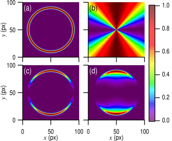
A typical image acquired in this type of experiment, either raw (through slice imaging), or, equivalently, mathematically inverted (through velocity map imaging), contains, in general, a set of “contributions” in the form of isotropic or anisotropic rings, by which we mean each of the possible processes or channels associated with a given ion or photoelectron. Typically, a “channel” is characterized by ions or photoelectrons with a given velocity (or center-of-mass kinetic energy) distribution, which, on the image, can be modeled, for instance, by a radial Gaussian function of the form
R(r) =exp "
−4 ln 2
r−rc
σc
2#
, (1)
wherercis the radial distance from the center of the image andσcis the full-width-at-half-maximum
71
(FWHM) of the contribution. Figure1a shows an example of such a contribution in the form of an
72
isotropic ring with parametersrc=40 andσc=3 in units of pixels (px) of the CCD camera, which are
73
The angular distribution (anisotropy) of charged particles for a given radius provides additional
information on the nature of the channel. In the case of inversion symmetry, the anisotropyAcan be
written as
A(α)∝1+
∑
n
β2nP2n(cosα) (2)
whereαis the angle between the polarization axis of the electric field and the considered direction and
75
ntakes maximum values of 1 and 2 for one-photon and two-photon processes, respectively. Legendre
76
polynomials,P2n(cosα), represent a complete angular basis set, which has the advantage that only few
77
terms in Eq.2are generally sufficient to describe the ring anisotropy. A 2D plot of this function using
78
β2=2 andβ2n>2=0 is shown in Fig.1b.
79
A channel can be fully described by the product of the velocity and angular distributions, 80
R(r)A(α). Figure1c shows the result of the product of the 2D radial and angular representations
81
shown in Figures1a and 1b. The corresponding raw velocity map image can be simulated by applying
100 50
0
x (px) 100
50
0
y
(px)
100 50
0
x (px) 100
50
0
y
(px)
(a)
(b)
(c)
(d)
1.0
0.8
0.6
0.4
0.2
0.0
Figure 1.2D representation of (a) the radial distribution given by Eq. (1) with parametersrc=40 px andσc=3 px, (b) the angular distribution given by Eq. (2) usingβ2=2 andβ2n>2=0, (c) the product of the radial and angular distributions shown in (a) and (b), and (d) the corresponding Abel projection of (c).
82
the Abel projection [4] and the result is shown in Figure1d. This simulation of a VMI image has been
83
obtained assuming cylindrical symmetry on the 3D distribution, for which Figure1c is the central slice.
84
Multichannel processes lead to imagesIwith a collection of contributionsCilike the one described
above. In the case that the different contributions do not interfere with each other, the experimental signal can be described by the following sum:
I=
∑
i
aiCi, (3)
whereai is the amplitude of each contribution. In the case that interferences occur, Eq. (3) would
85
include additional interference terms. 86
the case of a contribution which appears from the depopulation of an excited state (described by an exponential-type growth of the amplitude factor), the temporal behavior can be modeled as
Γ(t) =Ir(t)⊗
H(t−t0)×
1−e−
(t−t0)
τ
, (4)
whereH(t)is the Heaviside step function andIr(t)is the apparatus function, which typically depends
87
on the duration of the laser pulses. The variablet0represents the central pump-probe delay time for
88
which the contribution appears, andτis the time constant of the exponential.
89
Therefore, the complete 3D description of a contributionCi(r,α,t)can be written as
Ci(r,α,t) =Ri(r)Ai(α)Γi(t). (5)
This contribution is illustrated in Figure2.
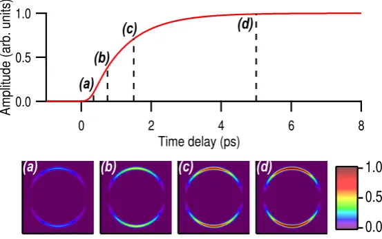
8 6
4 2
0
Time delay (ps) 1.0
0.5
0.0
Amplitude (arb. units)
(a)
(b)
(c)
(d)
(a)
(b)
(c)
(d)
1.0
0.5
0.0
Figure 2. Temporal evolution of a contribution with a temporal behavior described by Eq.4with τ=1 ps,t0=250 fs and whereIr(t)is a Gaussian function with a FWHM of 300 fs. The images shown below correspond to the contribution depicted in Figure1at selected delay times.
90
In the particular case described above, time appears completely decorrelated from the other dimensions. However, in a more general case, some parameters of the radial or angular distributions can change with time. For example, the anisotropy can relax, the central position of the ring can shift or its width can vary. Hence, the contribution can be written in a more general way as:
Ci(r,α,t) =Ri(r,t)Ai(α,t)Γi(t) (6)
where now bothRandAbecome functions that depend on time. TheΓi(t)function could be contained
91
in the functional form of Ri or Ai, but we have chosen to keep it explicitly written in Eq. 6for
92
convenience. This formalism can be generalized in a straightforward manner to any image scan as a 93
function of an arbitrary observable, such as wavelength or temperature, for example, thus extending 94
the dimensionality of the problem. 95
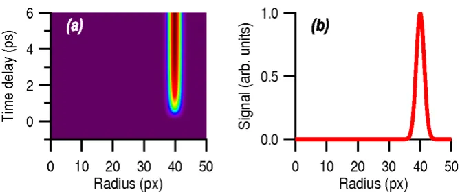
In some cases, the study of the dependence of the velocity distribution with time can be sufficient to extract all the relevant information of the pump-probe VMI experiment, with no additional insight
to be gained from the anisotropy. In this situation, Eq.6can be angularly integrated and the signal
originating from a given contribution becomes
in the case that the velocity distribution changes with time, or
C2D(r,t) =R(r)Γ(t), (8)
if it does not.
Figure 3.(a) 2D representation of the signal shown in Figure2angularly integrated as a function of radius and time. (b) Velocity distribution (in pixels of the CCD camera) extracted from (a) at a fixed delay time of 5 ps.
96
A 2D representation (angularly integrated) of the contribution considered in Figure2is displayed
in Figure3a. Figure3b shows the velocity distribution (in pixels of the CCD camera) corresponding
to a delay time of 5 ps. The amplitude and shape of the 2D and 3D representations can be directly compared through the angular integration
C2D(r,t) =
Z π
−π
r2|sin(α)|
2 C(r,α,t)dα. (9)
In the case that the non-zero anisotropy parametersβ2nare limited to the first few orders, an
alternative method to keep the 3D information consists of angularly integrating the VMI image in
steps of∆θ(10◦for example) providing a set of 2D maps as follows
Cθn
2D(r,t) =
Z θn+∆θ/2
θn−∆θ/2
r2|sin(α)|
2 C(r,α,t)dα. (10)
In that case, the 3D fitting procedure is employed using thenmaps ofCθn
2D(r,t). This last method
97
provides the same results as the direct 3D method (Eq.6) but tends to reduce the data size through the
98
integration step. This can be employed in case of slow convergence of the optimization algorithm. 99
2. Numerical fitting procedure 100
The quality of a 1D least-squares fitting procedure is related to the possibility to produce a 1D 101
vector, constructed from a parameterized functional form, to fit a 1D data vector. The most commonly 102
available fit procedures are developed for one dimension. Typically, the routine optimizes a set of 103
parameters,pm, of a user-defined functionalF(x;pm), which minimizes the global difference between
104
the fit and the data for all values of thexvariable.
105
A multidimensional fit can be performed using the same procedure by comparing each element 106
of the matrix generated by the initial guessF(x1,x2, . . . ,xn;pm)with the corresponding element in the
107
data matrix, and searching for a global minimization (in our case, the minimization algorithm employed 108
is a Levenberg-Marquardt nonlinear regression method [35–37]). In this sense, the multidimensional 109
fit method can be realized using the standard 1D procedure for which all the elements of thenD matrix
110
the use of invertible functions that convert ann-dimensional matrix into a single vector. The method 112
of choice is to construct a 1D vector that contains, in queue, all the columns of the matrix and all 113
the images of the sequence. This same conversion procedure is applied to both simulated and data 114
matrices before and after the used of the optimisation algorithm. 115
A second issue concerns the choice of coordinates. Whereas the formalism of Sec.1is written
116
in polar coordinates (r, the distance from the center, and α, the angle from the vertical axis), the
117
experimental signal is normally recorded using a widely available 2D CCD camera with pixels that are 118
well defined in cartesian coordinates. We propose to relate the polar and cartesian coordinates through 119
the advantageous complex representation: 120
reiα=i(x−c
x)−(y−cy)d (11)
where (cx,cy) are the coordinates of the center of the image anddis a distortion parameter of the image
121
(different from unity in the case that the pixels are not square). In this way,αis defined from−πto
122
πwith respect to the vertical-up semi-axis, which is taken as the origin angle. In the case that the
123
polarization axis of the laser does not match with the vertical lines of the camera but holds an angleδα
124
with it, it can be taken into account by multiplying Eq.11by exp(iδα). We choose to fixα=0 in the
125
singular case ofr=0 (i.e. cxandcyare integers). The images shown in Figures1and2are constructed
126
using this conversion from polar to cartesian coordinates. 127
As was mentioned before, it is common that VMI images are recorded as a function of an 128
experimental variable of interest. Examples of this are pump-probe time delay , laser wavelength , 129
polarization angle, temperature or sample density. This implies that a standard experiment performed 130
in this way can produce tens or hundreds of images (for instance, 640×480 pixels, with 12-bit dynamic
131
range). With the conditions above, a single experiment with 100 images produces 50 MB in a stack of 132
3D data. Since the larger the size of the data stack, the slower the convergence of the minimization 133
algorithm, it is important to find either symmetries or constraints that can reduce the number of data 134
points. For example, in the case of symmetric Abel-inverted images, it is possible to work only with a 135
square quarter of the image (corresponding to, say, 240×240 pixels). The image size can be further
136
reduced performing an (n×n) local integration, which reduces the size by a factorn2, although it can
137
only be used if the spatial resolution required is not lower thann.
138
The description of a 3D functional necessarily requires a large number of parameters. The shape 139
of each contribution along each axis and the correlations between them need to be considered. In the 140
case of a time-resolved VMI experiment, the simplest contribution requires at least 6 parameters: one 141
global amplitude, two temporal parameters (central position and time constant), two radial parameters 142
(position and width) and one angular parameter (β2in Eq.2). Indeed, the number of parameters
143
increases with the number of observed channels. However, some parameters can be common for 144
several contributions such as the origin of time which usually corresponds to the temporal overlap 145
between the pulses and the width of some of the peaks that can be related to the apparatus function. 146
Initial guesses for the parameters must be carefully chosen in order to reduce the convergence 147
time. A step by step procedure is proposed as follows. In order to find reasonable initial values for 148
the parameters and test the functionals, prospective low resolution fits are previously realized with 149
an(n×n)binning accompanied with a reduction of the number of images per time interval, so that
150
the convergence time is reduced to a few minutes. The introduction of the contributions has to be 151
performed stepwise, starting with the most intense one. A functional form for this main contribution 152
is proposed, either empirically or from theoretical arguments, using parameters that can be estimated 153
from visual inspection of a few images. Depending on the quality of the fit (looking at the residual), 154
the functional can be improved. Then the other contributions are introduced one by one using the 155
same strategy. Finally, the final adjustment is realized by removing the binning and considering all the 156
3. Case example: Analysis of a femtosecond pump-probe VMI experiment 158
In this section, we illustrate the strategy described in Secs. 1 and 2 to the analysis of an
159
experimental image sequence obtained in a femtosecond pump-probe VMI experiment. We take 160
as an example the photodissociation of CH3I in theB-band, using a 201.2 nm femtosecond pump laser
161
pulse where the appearance of the I*(2P1/2) fragment is probed by (2+1) REMPI with an ultrashort
162
305 nm laser pulse [38]. The dissociative mechanism of CH3I in theB-band is relatively simple and
163
consists of an electronic predissociation process [39–42]. The absorption of one pump photon at 164
201.2 nm excites the CH3I molecule from the electronic ground state into a bound Rydberg state in the 165
ground vibrational state (000transition). This Rydberg state is crossed by a repulsive potential energy
166
surface (PES) belonging to theA-band, which correlates with CH3and I*(2P1/2) fragments [43]. The
167
initial population in the Rydberg state can be transferred into the repulsive PES with an efficiency 168
that depends on the coupling between the two surfaces. Once the transfer is done, the dissociation 169
of the molecule occurs in tens of femtoseconds producing CH3and I*(2P1/2). When the iodine atom
170
is created, it can be resonantly ionized by the probe pulse using a (2+1) REMPI scheme. The ionized 171
fragments are accelerated by an external static electric field and focalized onto a microchannel plate 172
coupled with a phosphor screen. The VMI-image (i.e.the Abel projection of the Newton sphere) is
173
then recorded by a 12-bit Peltier cooled CCD camera. A set of images is recorded as a function of the 174
pump-probe delay time. Each image is numerically inverted using an Abel inversion procedure [28] 175
to retrieve the 3D velocity distribution of fragments as shown in Figure4a and4c. See Ref. [38] for
176
further details. 177
As usual in VMI experiments, each image contains information about the fragment velocity 178
and angular distributions. Typically, a number of well defined rings representing the velocity-angle 179
distribution of given photodissociation channels can be observed in the images. In the present case, the 180
time and anisotropy evolution of one ring is clearly observed in the sequence of images. The amplitude 181
of the signal of the ring depends on the number of iodine ions that are detected. The width of this 182
contribution directly depends on the rovibrational temperature of the initial molecule and that of the 183
CH3co-fragment, convoluted by the imaging apparatus resolution. The exact shape of the curve of
184
the velocity distribution can be quite complicated; nevertheless, it can be reasonably approximated by 185
Boltzmann, Gaussian or Lorentzian functions. In this experiment the main ring can be modeled as 186
the sum of two Gaussian functions which represents the CH3co-fragment in the ground vibrational
187
state (ν=0) and with one quantum of vibrational excitation in the symmetric stretch mode (ν1=1).
188
The temporal behavior expected for the relaxation of population can be modeled by an exponential 189
function, as shown in Eq.4. The anisotropy of a single linearly polarized photon phenomenon can
190
be described by the second Legendre polynomial, consideringβ2as the only non-zero coefficient in
191
Eq.2. The value ofβ2primarily depends on the angular nature of the transition,i.e. whether the 192
transition dipole moment is parallel or perpendicular to the dissociation axis. For the parallel case, 193
β2>0 with a maximum value ofβ2=2; for the perpendicular case,β2<0 with an extreme value of
194
β2=−1. Both theoretical calculations and experiments for CH3I have shown that the transition from
195
the electronic ground state to theB-band is of perpendicular nature. The observed final anisotropy,
196
measured through angular distributions of the fragments, can differ from the limiting cases of parallel 197
(β2 = 2) or perpendicular (β2 = −1) anisotropy, mainly because rotation of the molecule prior to
198
dissociation tends to blur the angular preference. This is especially relevant in the case of an indirect 199
dissociation process if the time scales are similar or slower than molecular rotation. 200
Inspection of a few experimental images of the sequence shows that the anisotropy does evolve in
this way [38],i.e.images taken at earlier delay times show a more pronounced anisotropy than those
of the angular parameters is a function of time. The functional form of the loss of anisotropy with time
is not known. An exponentially decreasing modulus of theβ2parameter is proposed as:
β2(t) =β20+∆β2e
−(t−t0)
τβ2 , (12)
where β20 is the asymptotic anisotropy parameter, β20+∆β2 is the amplitude of the anisotropy
201
parameter att=t0andτβ2 is the relaxation time. Some theoretical work has been dedicated to define
202
the final value ofβ20for a dissociation process that is either parallel or perpendicular, considering the
203
dissociation time [44,45]. Those theoretical models are based on the rotation of the excited wave packet 204
prior to dissociation. Although no predictions are available on the relaxation time, it can be estimated 205
to be in the picosecond time scale. 206
The complete 3D function that was employed to describe the main contribution (anisotropic ring)
on theB-band photodissociation of CH3I can be written as follows:
C1(r,α,t) =Γ(t)×β2(t)P2(cosα)×[R1,a(r) +eR1,b(r)]. (13)
whereR1,a(r)andR1,b(r)are the radial contributions corresponding to CH3fragments in the two
207
vibrational states mentioned above, andeis the fraction of the population of CH3inν1=1.
208
Femtosecond pump-probe VMI images contain, in general, some other low intensity secondary 209
contributions, which can arise from different mechanisms, as for example, absorption of two pump 210
photons, relaxation of the molecule over another state which has lower absorption probability, detection 211
by non-resonant ionization or background gas contamination. The secondary contributions have to be 212
considered in the fitting procedure if they are overlapped with the contribution or contributions of 213
interest. In fact, a good reproduction of the secondary signals allows the isolation of the contribution 214
of interest from the rest by subtraction of the previously fitted secondary signals. If these secondary 215
contributions are neglected, then an error is generated in the fit with a magnitude corresponding to the 216
sum of the secondary signals in the spatial overlap region. 217
In the present case example [38], the secondary contributions can be grouped into two classes. 218
The first one appears in a broad range of velocities, is characterized by an asymmetric temporal 219
shape and presents a complex anisotropy. This contribution appears quickly at short delay times and 220
then slowly disappears. The second contribution has more localized velocities around the region 221
of the contribution of interest (main ring). Moreover, it has a temporal evolution similar to the 222
main contribution. Additionally, the secondary contributions show anisotropies which require the 223
consideration of bothβ2andβ4terms in Eq. 2.
224
In what follows, the specific results of the 3D fitting procedure applied to the mentioned case 225
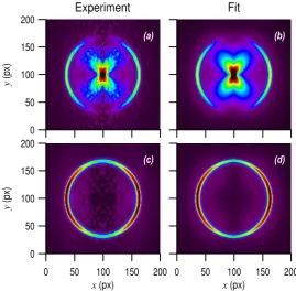
example are presented. Figure4shows two typical images, out of the sequence of 80 images recorded,
226
fitted at short (120 fs) and asymptotic (10 ps) delay times. In order to remove the standard 3-4 pixel 227
region of noise produced by the Basex inversion around the central column of the images [28], the fit 228
has been carried out 4 pixels away from the central axis. Those points are thus removed from the fitted 229
and measured images shown in Figure4. Additionally, some of the mathematical functions used in the
230
fitting procedure present a singularity at the center of the images. In order to avoid the singularities, a 231
10 pixel circle was set to zero in the fitted and measured matrices. The elimination of these areas of the 232
images does not represent any problem in the analysis, since all the relevant contributions are far away 233
from the center. 234
The advantage of the 3D fitting procedure is that the anisotropy is considered. In the present case, 235
the main contribution (ring) starts with a pronounced anisotropy (of perpendicular character), with 236
the ion signal concentrated at the equator of the images, and later the ring evolves to become more 237
isotropic. The anisotropy parameters of Eq.12obtained from the fit for this main contribution are
238
β20 =−0.50±0.03,∆β2=−0.51±0.03 andτβ2 =1.26±0.13 ps. Therefore, the fitted anisotropy at
239
t=t0isβ2(t=t0) =−1.01±0.06, which is characteristic of a purely perpendicular transition.
200
150
100
50
0
y
(px)
200 150 100 50 0
x (px)
200
150
100
50
0
y
(px)
200 150 100 50 0
x (px)
(a) (b)
(d) (c)
Experiment
Fit
Figure 4.(a)and(c)Experimental Abel inverted VMI images recorded for the I*(2P
1/2) fragment at 120 fs and 10 ps delay times, respectively.(b)and(d)Corresponding fitted reconstructed images.
The two secondary contributions are visible in the experimental images shown in Figure4. The
241
first can be clearly seen at the center of the image shown in Fig.4a; the second is appreciated at the
242
vicinity of the main ring in Fig.4c. These secondary contributions, together with the main contribution,
243
can be distinguished in a more clear way in the velocity distributions shown in Fig.5at two delay
244
times. 245
The time evolution of the velocity distribution can be well represented by angular integration of 246
the images, as shown in Figure6. The main contribution (ring) has been fitted in velocity (pixels) using
0.12
0.10
0.08
0.06
0.04
0.02
0.00
Signal (arb. units)
100 80 60 40 20 0
Radius (px)
1.0
0.8
0.6
0.4
0.2
0.0
100 80 60 40 20 0
Radius (px)
(b)
(a)
Figure 5.I*(2P1/2) fragment velocity distributions (in pixels) at (a) 120 fs and (b) 10 ps delay times. The experimental data (
-
), the fitted total (-
) and the fitted different contributions (main (· · ·
) and secondary (- -
and·−
)) are shown.247
the sum of two Gaussian functions, which have the same width (5.27±0.04 pixel) as indicated in Ref.
248
[38]. The central position has been found to be at 69.9±0.5 px for the main peak and at 65.7±0.5 px for
249
the minor shoulder with an amplitudee=0.147±0.002. As was indicated above, the main peak and
the shoulder are assigned to dissociation channels yielding CH3(ν=0)and CH3(ν1=1), respectively. 251
Figure 6.2D representation corresponding to the angular integration of the I*(2P1/2) fragment image sequence as a function of the delay time.
252
The temporal evolution of the secondary contribution appearing in the center of the images has 253
been fitted using a 400±50 fs Gaussian convolution of a 1.7±0.1 ps exponential decay, and that of
254
the other secondary contribution, which is closer to the main contribution, can be modeled with a 255
functional form as in Eq.4with a time constant ofτ=1.48±0.05 ps.
256
The temporal behavior of the contribution of interest isolated from the secondary contributions 257
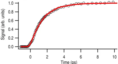
is shown in Figure7as a 1D transient. The data points shown in this figure have been obtained
258
through subtraction of the fitted secondary contributions from the experimental measurement. Then 259
the resulting signal has been fully integrated angularly and radially integrated over the region of 260
interest. An exponential-type growth (Eq.4) with a time constant of 1.54±0.04 ps for this particular
1.0
0.8
0.6
0.4
0.2
0.0
Signal (arb. units)
10 8 6 4 2 0
Time (ps)
Figure 7.1D transient for the amplitude of the main contribution as a function of time. (◦) experimental data and (
-
) fit. See text for more details.261
case has been found from the fit. A set of measurements has been carried out, which allows the 262
evaluation of the statistical error. The time constant thus obtained has been found to be 1.5±0.1 ps, as
263
shown in Ref. [38]. 264
4. Conclusions 265
A multidimensional fitting methodology has been developed for the full analysis of time-resolved 266
velocity map image sequences obtained in femtosecond pump-probe photodissociation experiments. 267
The key advantage of the method consists of its capability to distinguish the different overlapped 268
contributions present in the set of images corresponding to different reaction channels of interest from 269
can be cleanly isolated from the secondary signals by filtering secondary contributions from the data 271
matrix. It must be noticed that the Abel projection can be implemented to fit recorded images directly, 272
in which case no previous requirements on inversion symmetry are necessary. 273
The present multidimensional fitting procedure has been applied to the analysis of a set of images 274
corresponding to the predissociation dynamics of CH3I in the origin of the B-band detecting the
275 I*(2P
1/2) fragments by 2+1 REMPI. Additionally, this methodology has been applied successfully to the
276
analysis of other dissociation channels of vibrationally excited CH3I in theB-band, and in theA-band,
277
both for the monomer and dimer species. 278
This multidimensional fitting concept applied in the present case to a set of velocity map images as 279
a function of time can be easily extended to other variables, like laser intensity, wavelength, temperature 280
or pulse duration. It can also be adapted to other types of signal detection, like fluorescence. In addition, 281
there is no conceptual problem to extend the fitting procedure tondimensions, the only limitation
282
being computational time restrictions to analyze ann-dimensional matrix.
283
Acknowledgments: This work has been supported by the Spanish Ministry of Economy and Competitiveness 284
(grants CTQ2015-65033-P and CTQ2016-75880-P). This research has been carried out within the Unidad Asociada 285
Química Física Molecular between Departamento de Química Física I of UCM and CSIC. The facilities provided 286
by the CLUR (Centro de Láseres Ultrarrápidos) are gratefully acknowledged. 287
Conflicts of Interest:The authors declare no conflict of interest. 288
References 289
1. D. W. Chandler and P. L. Houston, “Two-dimensional imaging of state-selected photodissociation products 290
detected by multiphoton ionization,” J. Chem. Phys.87,1445 (1987). 291
2. A. T. J. B. Eppink and D. H. Parker, “Velocity map imaging of ions and electrons using electrostatic lenses: 292
Application in photoelectron and photofragment ion imaging of molecular oxygen,” Rev. Sci. Instrum.,68, 293
3477 (1997). 294
3. J. A. Davies, J. E. LeClaire, R. E. Continetti and C. C. Hayden, “Femtosecond time-resolved 295
photoelectron-photoion coincidence imaging studies of dissociation dynamics,” J. Chem. Phys. 111,1 296
(1999). 297
4. B. J. Whitaker,Imaging in Molecular Dynamics. Technology and Applications(Ed. Cambridge Univeristy Press, 298
Cambridge, 2003). 299
5. J. Ullrich, R. Moshammer, A. Dorn, R. Dörner, L. Ph. H. Schmidt, H. Schmidt-Böcking, “Recoil-ion and 300
electron momentum spectroscopy: reaction-microscopes,” Rep. Prog. Phys.66,1463 (2003). 301
6. M. N. R. Ashfold, N. H. Nahler, A. J. Orr-Ewing, O. P. J. Vieuxmaire, R. L. Toomes, T. N. Kitsopoulos, I. A. 302
Garcia, D. A. Chestakov, S.-M. Wu and D. H. Parker, “Imaging the dynamics of gas phase reactions,” Phys. 303
Chem. Chem. Phys.8,26 (2006). 304
7. I. V. Hertel and W. Radloff, “Ultrafast dynamics in isolated molecules and molecular clusters,” Rep. Prog. 305
Phys.69,1897 (2006). 306
8. A. I. Chichinin, K.-H. Gericke, S. Kauczok, C. Maul, “Imaging chemical reactions - 3D velocity mapping,” 307
Int. Rev. Phys. Chem.28,607 (2009). 308
9. R. de Nalda, J. G. Izquierdo, J. Dura and L. Bañares, J. Chem. Phys.126021101 (2007). 309
10. K. L. Wells, G. Perriam and V. G. Stavros, J. Chem. Phys.130074308 (2009). 310
11. R. Spesyvtsev, O. M. Kirkby, M. Vacher and H. H. Fielding Phys. Chem. Chem. Phys.14, 9942–9947 (2012). 311
12. R. Spesyvtsev, O. M. Kirkby and H. H. Fielding, Faraday Discuss.157165–179 (2012) 312
13. R. de Nalda, J. Durá, J. González-Vázquez,V. Loriot and L. Bañares, Phys. Chem. Chem. Phys., 2011, 13, 313
13295–13304 314
14. G. Gitzinger, M. E. Corrales, V. Loriot, R. de Nalda, L. Bañares J. Chem. Phys.136, 074303 (2012) 315
15. M. E. Corrales, G. Balerdi, V. Loriot, R. de Nalda, L. Bañares Faraday Discuss.,163, 447 (2013) 316
16. M. E. Corrales, V. Loriot, G. Balerdi, J. González-Vázquez, R. de Nalda, L. Bañares, A. H. Zewail Phys. Chem. 317
Chem. Phys.16, 8703 (2014) 318
17. G. Balerdi, J. Woodhouse, A. Zanchet, R. de Nalda, M. L. Senent, A. García-Vela, L. Bañares Phys. Chem. 319
18. O. M. Kirkby, M. Sala, G. Balerdi, R. de Nalda, L. Bañares, S. Guérin, N. Kaltsoyannis, H. Fielding Phys. 321
Chem. Chem. Phys,17, 16270 (2015) 322
19. D. Townsend, H. Satzger, T. Ejdrup, A. M. D. Lee, H. Stapelfeldt, and A. Stolow J. Chem. Phys.125234302 323
(2006) 324
20. S. Ullrich, T. Schultz, M. Z. Zgierski and A. Stolow Phys. Chem. Chem. Phys.,6, 2796-2801 (2004) 325
21. A. E. Boguslavskiy, O. Schalk, N. Gador, W. J. Glover, T. Mori, T. Schultz, M. S. Schuurman, T. J. Martínez, 326
and A. Stolow J. Chem. Phys.148, 164302 (2018) 327
22. O. Schalk, A. E. Boguslavskiy and A. Stolow J. Phys. Chem. A1144058-4064 (2010) 328
23. V. Loriot, A. Marciniak, L. Quintard, V. Despré, B. Schindler, I. Compagnon, B. Concina, G. Celep, C. Bordas, 329
F. Catoire, E. Constant and F. Lépine J. Phys. Conf. Ser.635012006 (2015) 330
24. V. Loriot, A. Marciniak, G. Karras, B. Schindler, G. Renois-Predelus, I. Compagnon, B. Concina, R Brédy, G. 331
Celep, C. Bordas, E. Constant and F. Lépine, J. Opt.19114003 (2017) 332
25. V. Loriot, G. Gitzinger and N. Forget Opt. Express 21 24879 (2013) 333
26. V. Loriot, O. Mendoza-Yero, J. Pérez-Vizcaíno, G. Mínguez-Vega, R. de Nalda, L. Bañares and J. Lancis. App. 334
Phys. B11767 (2014) 335
27. A. Marciniak, V. Despré, T. Barillot, A. Rouzée, M.C.E. Galbraith, J. Klei, C.-H. Yang, C.T.L. Smeenk, V. 336
Loriot, S. Nagaprasad Reddy, A.G.G.M. Tielens, S. Mahapatra, A.I. Kuleff, M.J.J. Vrakking and F. Lépine Nat. 337
Commun.67909 (2015) 338
28. V. Dribinski, A. Ossadtchi, V. A. Mandelshtam, and H. Reisler, “Reconstruction of Abel-transformable 339
images: The Gaussian basis-set expansion Abel transform method,” Rev. Sci. Instrum.73,2634 (2002). 340
29. G. A. Garcia, L. Nahon and I. Powis, “Two-dimensional charged particle image inversion using a polar basis 341
function expansion,” Rev. Sci. Instrum.75,4989 (2004). 342
30. C. Bordas, F. Paulig, H. Helm and D. L. Huestis, Rev. Sci. Instrum.672257 (1996). 343
31. M. J. J. Vrakking, “An iterative procedure for the inversion of two-dimensional ion/photoelectron imaging 344
experiments,” Rev. Sci. Instrum.72,4084 (2001). 345
32. C. R. Gebhardt, T. P. Rakitzis, P. C. Samartzis, V. Ladopoulos and T. N. Kitsopoulos, “Slice imaging: A new 346
approach to ion imaging and velocity mapping,” Rev. Sci. Instrum.72,3848 (2001). 347
33. D. Townsend, M. P. Minitti and A. G. Suits, “Direct current slice imaging,” Rev. Sci. Instrum.742530 (2003). 348
34. J. J. Lin, J. Zhou, W. Shiu and K. Liu, “Application of time-sliced ion velocity imaging to crossed molecular 349
beam experiments,” Rev. Sci. Instrum.742495 (2003). 350
35. D. W. Marquardt, “An Algorithm for Least-Squares Estimation of Nonlinear Parameters,” SIAM J. Appl. 351
Math.11,431 (1963). 352
36. Y. Bard,Nonlinear Parameter Estimation(Academic Press, New York, 1974). 353
37. N. R. Draper and H. Smith,Applied Regression Analysis (Wiley Series in Probability and Statistics)(John Wiley & 354
Sons Inc, New York, 1981). 355
38. G. Gitzinger, M. E. Corrales, V. Loriot, G. A. Amaral, R. de Nalda and L. Bañares, “A femtosecond velocity 356
map imaging study onB-band predissociation in CH3I. I. The band origin,” J. Chem. Phys.132,234313 357
(2010). 358
39. D. J. Donaldson, V. Vaida and R. Naaman, “Ultraviolet absorption spectroscopy of dissociating molecules: 359
Effects of cluster formation on the photodissociation of CH3I,” J. Chem. Phys.87,2522 (1987). 360
40. P. G. Wang and L. D. Ziegler, “Mode-specific subpicosecond photodissociation dynamics of the methyl 361
iodideBstate,” J. Chem. Phys.95,288 (1991). 362
41. J. A. Syage, “Predissociation lifetimes of the ˜B and ˜C Rydberg states of CH3I,” Chem. Phys. Lett.212,124 363
(1993). 364
42. A. P. Baronavski and J. C. Owrutsky, “Vibronic dependence of the ˜B state lifetimes of CH3I and CD3I using 365
femtosecond photoionization spectroscopy,” J. Chem. Phys.108,3445 (1998). 366
43. A. B. Alekseyev, H.-P. Liebermann, R. J. Buenker and S. N. Yurchenko, “Anab initiostudy of the CH3I 367
photodissociation. I. Potential energy surfaces,” J. Chem. Phys.126,234102 (2007). 368
44. C. Jonah, “Effect of Rotation and Thermal Velocity on the Anisotropy in Photodissociation Spectroscopy,” J. 369
Chem. Phys.55,1915 (1971). 370
45. J. R. Waldeck, M. Shapiro and R. Bersohn, “Theory of transient anisotropy in molecular photodissociation,” J. 371