Phase transitions in Virology
Ricard Sol´e,1, 2, 3 Josep Sardany´es,4, 5 and Santiago F. Elena6, 3
1
ICREA-Complex Systems Lab, UPF-PRBB, Dr. Aiguader 80, 08003 Barcelona, Spain.
2Institut de Biologia Evolutiva, CSIC-Universitat Pompeu Fabra, Passeig Maritim de la Barceloneta 37, 08003 Barcelona, Spain. 3
Santa Fe Institute, 1399 Hyde Park Road, Santa Fe NM 87501, USA.
4
Centre de Recerca Matem`atica (CRM); and Barcelona Graduate School of Mathematics (BGSMath). Edifici C, campus de Bellaterra, Cerdanyola del Vall`es, 08193 Barcelona, Spain.
5
Dynamical Systems and Computational Virology, Associated Unit Instituto de Biolog´ıa Integrativa de Sistemas (I2SysBio) - CRM
6Evolutionary Systems Virology Lab, I2SysBio, CSIC-Universitat de Val`encia, Catedr´atico Agust´ın Escardino 9, Paterna, 46980 Valencia, Spain.
Viruses have stablished symbiotic relationships with almost every other living organism on Earth and at all levels of biological organization, from other viruses up to entire ecosystems. In most cases, peacefully coexisting with their hosts, but in most relevant cases, parasitizing them and inducing diseases. Viruses are playing an essential role in shaping the eco-evolutionary dynamics of their hosts, and also have been involved in some of the major evolutionary innovations either by working as vectors of genetic information or by being themselves coopted by the host into their genomes. Viruses can be studied at different levels of biological organization, from the molecular mechanisms of genome replication, gene expression and encapsidation to global pandemics. All these levels are different and yet connected through the presence of threshold conditions allowing for the formation of a capsid, the loss of genetic information or epidemic spreading. These thresholds, as it occurs with temperatures separating phases in a liquid, define sharp qualitative types of behavior. Thesephase transitionsare very well known in physics. They have been studied by means of simple, but powerful models able to capture their essential properties, allowing to understand them. Can the physics of phase transitions be an inspiration for our understanding of viral dynamics at different scales? Here we review the best known examples of transition phenomena in virology and their simplest mathematical modeling approaches. We suggest that the advantages of abstract, simplified pictures used in physics are also the key to properly understand the origins and evolution of complexity in viruses. By means of several examples, we explore this multilevel landscape and how minimal models provide deep insights into a diverse array of problems. The relevance of these transitions in connecting dynamical patterns across levels and their evolutionary and clinical implications are outlined.
Keywords: Epidemics, molecular replicators, mutation, multi-level selection, quasispecies, recombination, self-assembly, phase transitions, virus evolutionary dynamics
I. INTRODUCTION
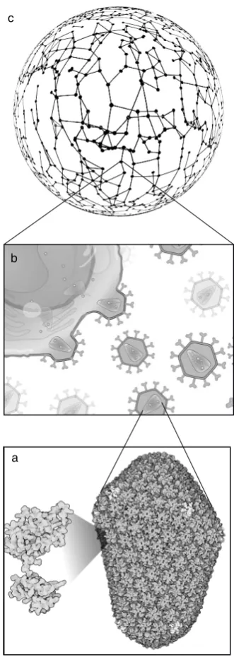
Researchers from different disciplines tend to study viruses at their favorite level of biological organization (Fig. 1). At the lowest scale of biological complexity, molecular virologists carefully characterize the mecha-nisms of viral replication and pathogenesis, the molecular interactions between viral proteins and among viral and host proteins, and how cells respond to infection by trig-gering diverse defense mechanisms. At the highest scale, ecologists and epidemiologists describe the incidence of viruses in their reservoir and potential novel hosts, and their spread among host populations and at the global level, including their impact on nutrient cycling. At each scale, what is considered as the ’host’ is different: single cells or tissues for molecular virologists, individuals for clinical virologists and plant pathologists, populations of hosts or even entire ecosystems for ecologists and epi-demiologists. Likewise, the ’virus’ unit upon which se-lection operates also differs among the levels of biological organization being studied: mutant swarms within indi-viduals, infected individuals in ecological studies or viral
lineages in phylogeography and epidemiological studies. But the ultimate host for any virus is always an individ-ual cell. It is inside the cell wherein the virus expresses its genes, kidnaps the cellular resources and manipulate structures to build the replication factories. Viral pro-teins and RNAs interact with a large number of cellular factors in order to block cell defenses, to ensure reproduc-tion, encapsidation and spread to neighboring cells. From there to colonize other tissues and organs, and from there to be transmitted to other susceptible hosts, to spread in the host populations and, ultimately, to reach diverse ecosystems.
Different selective pressures operate on viruses at each of the above levels. For example, whereas at the cellu-lar and within-organism levels fast replication may pro-vide competitive advantage to one strain over another, at the population level such strategy may not be optimal, as it jeopardizes transmission between hosts by immo-bilizing the infected host and thus effectively reducing the rate of transmission (Doumayrouet al. 2012). An-other remarkable example of seemingly opposed obser-vations: population-level human immunodeficiency virus
type 1 (HIV-1) phylogenies are mainly shaped by se-lective neutral epidemiological processes, implying that genealogy-based population genetic inferences can be useful to study the HIV-1 epidemic history and dating events (Lemey et al. 2006). In sharp contrast, HIV-1 phylogenies reconstructed from withhost sequences in-dicate the action of strong selective pressures imposed by the heterogeneity of cell types in which the virus can be replicated (Lemey et al. 2006). Indeed, the existence of within-host reservoirs of latently infected CD4+ T cells produces a delay in the evolutionary dynamics within single hosts. These delays can fundamentally change the dynamics of the virus transmission between individuals and, hence, have an impact at the epidemiological scale (Doekes et al. 2017). Therefore, while the general con-nection between the infection dynamics within a host and the population-level transmission dynamics of viruses is widely acknowledged, a comprehensive and quantitative understanding that would allow full integration of the two scales is still lacking.
There have been attempts to model multi-scale selec-tion for viruses. At most, studies have tried to model between-host transmissions as a function of within-host replication parameters (Coombset al. 2007; Mideoet al. 2008; Metzgeret al. 2011; Fenget al. 2012; Scholeet al. 2013; Shin and MacCarthy 2016; Doekeset al. 2017; Dor-ratoltaj et al. 2017), or tissue/organ colonization as an extension of within-cell replication events and interaction with host factors (Sardany´es and Elena 2011; Heldtet al. 2013; Kumbergeret al. 2016). Unfortunately, the former models usually ignore the inherent within-host complex-ity, while the latter never extend beyond the individual tissue or single host. Gonget al. (2015) identified seven challenges for developing multi-scale models of virus evo-lution:
1. Lack of models and data to elucidate the processes underlying transmission probabilities and bottle-necks. From the donor host side, how does infec-tiousness depend on virus load? From the recipient host side, initial infection depends on the dose (bot-tleneck), route of transmission, time of exposure, etc. Stochastic and spatial invasion models will of-fer insights if feed with the appropriate empirical data.
2. Heterogeneity within a single host. Many of the existing within-host models describe the host as a single population of target cells without any struc-ture. This is obviously not the case and heterogene-ity in cell type, spatial structure, susceptibilheterogene-ity and immune response will all play important roles in shaping infection dynamics.
3. Fitness landscapes may be highly dynamic and variable between host types. Very little is known about the topography of the fitness landscapes into which viral populations evolve. Evidences suggest they may be rugged but also contain some degree
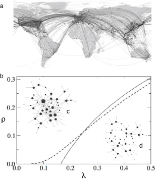
a b c
FIG. 1: The multiple levels of virus dynamics. Here only three key examples are displayed, namely (a) molecular assembly (b) virus-cell infection, and (c) social network of individual hosts, represented as a graph with links indicating potential transmissions. Between these levels, other intermediate scales such as tissue/organ levels need to be considered.
of neutrality (Kouyoset al. 2012; Lali´c and Elena 2015). Landscape’s topography may be strongly affected by the cell types and immune responses, with epistasis (Elena et al. 2010) and antagonis-tic pleiotropy being essential components (Cervera
et al. 2016). Indeed, it has been recently
ob-servations in virus evolution. Instead, it has been suggested that an adaptive multiscape (Catal´an et al. 2017), or a time-fluctuating adaptive seascape (Mustonen and L¨assig 2009), may provide a much better representation.
4. Current models do not easily incorporate high-throughput next-generation sequencing (NGS) data. Empirical studies have demonstrated that during acute and chronic infections, RNA viruses generate massive amounts of genetic variability (Domingo et al. 2012). In some cases, this ge-netic diversity is transmitted, in some other not. NGS provides valuable information to assess the size of bottlenecks and the spread of resistance variants. Furthermore, quantitative methods have been established at the epidemiological level, or us-ing global level phylogeography analyses, typically based on consensus sequences, but there seem to be no well-established methods for analysis of NGS data at this level, thus missing the opportunity to link within- and between-individual diversity with epidemiological processes.
5. Ignoring superinfectiona has greatly simplified
modeling efforts. However, it is not clear when this approximation should be valid. Superinfection is known to be important in many viruses,e.g. HIV-1, increasing viral load and hastening progression to AIDS (Korenromp et al. 2009).
6. The distinction between within- and between-host dynamics can be easily made. However, the fact that both of these scales involve further nested lev-els has been often neglected. While multi-scale models at the population level are common, these models ignore the within-host components. This lack of integration of within-host levels of complex-ity, so far, resulted from the lack of information in vivo. Fortunately, this limitation is being overcome with NGS and the development of models that take into account cellular processes (e.g., Loverdoet al. 2012).
7. What approaches should be used to link processes across scales? modeling multi-scale processes in full mechanistic detail, or even simulating such mod-els, is unrealistic. One possibility is to come up with ways of extracting the essential features of lower-scale models to embed them into higher-scale models efficiently (Mideo et al. 2008). An ap-proach that has been successfully taken is to sep-arate timescales, which essentially sepsep-arates mod-els that may be used at different scales. Following
a Superinfection refers to the process in which an already infected
host becomes secondarily infected by a different virus or a differ-ent strain of the same virus.
this philosophy, Park et al. (2013) used Markov chain modeling at the within-host level embedded into a stochastic branching process for between-host transmission. The challenge is to develop bet-ter methods for incorporating multiple scales into a single framework.
As complex adaptive dynamical systems, viruses ex-perience critical phase transitions at different levels of organization (Sol´e and Elena, 2019). These critical tran-sitions involve a sudden change in the dynamical behav-ior or the internal structure of the system. At the lowest molecular level, the concept of critical points at phase transitions have been used to describe process such as the assembly and disassembly of viral particles (Dhar-mavaramet al. 2017), the error threshold associated to the highly mutagenic replication of viral genomes (Eigen 1971), the spread of perturbations across host protein-protein and regulatory networks induced by viral factors (Bosqueet al. 2014), and the agglomeration of viral par-ticles to form pseudo-crystal structures which may op-erate as units of selection (Cuevaset al. 2017). At the individual patient level, coordinated changes in expres-sion levels of host proteins linked into functional modules may act as early-warning signals for the critical transi-tion between healthy and disease stages during infectransi-tion (Liuet al. 2012). Finally, at the epidemiological level, spread of a viral disease in a scale-free network formed by connected populations of susceptible host show com-plex dynamical behavior and phase transitions from non-epidemic to non-epidemic stages associated with the existence of highly connected hubs (Barth´elemyet al. 2005; Bal-can and Vespignani 2011). So far, models connecting phase transitions at different levels have not been pro-posed. Likewise, no model has been brought forward to explore whether transitions at one level may results from the dynamical properties of the levels below, especially whether the role of natural selection at each level may interplay with criticality.
ex-a
b
c
d
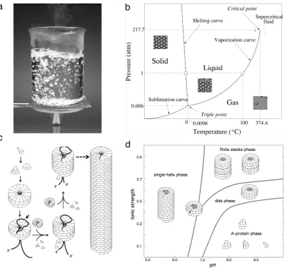
FIG. 2: Phase transitions in both physics and virus dynamics involve marked qualitative changes. An example is (a) the boiling of water, where the two phases (liquid and steam) coexist. For different values of temperature and pressure, a phase diagram (b) reveals three basic phases are separated by well-defined critical curves. The molecular organization of viral capsids is also sharply affected by key parameters. An example is the formation of TMV that takes place by self-assembly of coat proteins (c) leading to long rods. But such process and the final nature (phase) of the self-assembly process is sharply controlled by physicochemical parameters, such as pH or ionic strength. This pair of parameters allow displaying a phase diagram (d) that also exhibits transition lines between different configurations.
istence of these critical organization thresholds that can be clearly identified by means of the so-called bifurca-tions. Readers less interested in mathematical details can jump over the next section without losing the main messages.
II. PHASE TRANSITIONS: SIMPLE MODELS EXPLAIN COMPLEX CHANGES
Phase transitions are introduced in this paper with the aim of providing a proper framework to understand the nature of change in virology. By change we refer to the
qualitative dynamical and structural shifts of organiza-tion of complex systems. The term phase transiorganiza-tion was
coined to describe the sudden shift between states of mat-ter, but has been since then generalized to many other domains (Sol´e, 2011). An example is the phase change from ice to liquid water or from water to steam, as shown in Fig. 2a . Each phase is defined by some state that is uniform within its domain in the phase diagram, which essentially tells us which phases are stable under what conditions. Such properties can rapidly change close to the boundaries between phases. Figure 2b shows a clas-sical example, namely the transition from liquid water to steam. Within a given phase, no major differences can be seen beyond smooth quantitative changes. As an example, when water is heated from 2 oC to 25 oC
changes slightly (by just 2 %) while it decreases 1600-fold as boiling temperature is reached. In other words, a slight change close to the transition point drives a very large, abrupt change in density. Such abrupt transition is termed ”first-order” and is also observed in the melt-ing of ice. This occurs also in other diverse systems, such as polymers and other materials experiencing qual-itative structural re-arrangements (Dill and Bromberg 2012), abrupt climate change (see Sol´e 2011 and refer-ences therein) or ant colonies exploring their environ-ments (Beekman et al. 2001; Pi˜nero and Sol´e 2019). In all these systems it is possible to define a phase dia-gram showing the parameter values at which the different states (phases) are found. Now, instead of temperature and pressure, the axes can include, for example, molec-ular concentrations or strength of ionic forces, which af-fect the kinds of capsid assembly for the tobacco mosaic virus (TMV) (Fig. 2c-d). The process of virus assembly requires the formation of rods (Fig. 2c) which is affected by key external parameters defining a space of shapes (Fig. 2d). The structures shown here are the dominant ones in each phase (Klugg 2010).
A different class of transition, known as a second-order phase transition, involves a qualitative change as well but this change occurs in a smooth manner as parame-ters vary. This is the case for example in the behavior of ferromagnetic materials: when a magnet is heated, it initially maintains its magnetization, which decays until it vanishes altogether at a critical temperature Tc. In
these transitions, remarkably rich behavior can be ob-served, including both very high variance in both struc-tural and dynamical traits. wide fluctuations in the mea-sured macroscopic properties (such as magnetization) are observed as we approach criticality (the phase transition point) where the variance diverges. For this example, we have a microscopic description that allowed to for-mulate a simple model capable of capturing most rele-vant features of the real transition. This is the so called
Ising modelor, as physicist Nigel Goldenfeld calls it, ”the
Drosophila model of statistical mechanics”.
A magnet can be imagined as a lattice of units (atoms) each one describable as some kind of magnet itself, with two possible orientations (or ”spins”): up and down. Mathematically, that means that we have a collection of
Nunits whose states are indicated asSk, located on a
ge-ometric grid and having two possible states, saySk =−1
and Sk = +1. From quantum mechanical arguments, it
is known that the lowest energy state (and thus the more likely) is the one where nearest atoms have the same spin states (with some probability). If the two types of spins are indicated as +1 and −1, the difference between the number of up spins (N+) and down spins (N−), defines
the global magnetization M, i.e. M =N+−N−. This
value gives the capacity of the magnet to attract other ferrous materials. As temperature grows, the coupling between spins becomes less and less strong. If tempera-tureT is below a critical value, labeled Tc, interactions
among nearest spins would favor a dominant direction.
Assuming that the system started from a random ini-tial condition, the outcome of spin-spin interactions is one of two possible macroscopic ordered states: either a majority of up spins or the alternative dominated by down spins. However, ifT > Tc, disorder wins, and spins
essentially behave randomly. This is thus a transition between two equally likely ordered states whereM 6= 0 and a disordered phase withM = 0. Within each of the two phases, all measurable properties change smoothly.
The previous observations can be captured using a mi-croscopic model (the so called Ising model) that involves defining anenergy function H given by the sum (Chris-tensen and Moloney, 2005)
H =−1 2
X
hi,ki
JSkSi, (1)
whereJ is a coupling constant that weights the strength of spin-spin interactions. The brackethi, kiindicates that the pairs are restricted to nearest neighbors. As defined, we can see that energy decreases (as it occurs with any spontaneous phenomenon) when SiSk = 1, i.e. when
both spins are oriented in the same direction. Along with this energy function, a set of rules is needed to introduce changes into the state of the units as they interact under a given temperature. In a nutshell, we need probabilities of transitionP[Si→1−Si] for every chosen unitSi
be-tween the two possible states, that include on one hand the effect of temperature (the higher, the weaker the in-teraction) and, on the other hand, the set of neighbors of the chosen unit. The larger the fraction of neighbors pointing in the same direction, the more likely that our unit will follow them. It can be shown (Sol´e 2011) that one simple way of implementing this probability is:
P[Si→1−Si] =
1
1 + exp(∆H/kT), (2) where ∆H indicates the change in energy associated to the spin flip. It can be easily shown that this transition probability properly behaves as expected: it will be close to 0.5 (coin toss) for high temperatures while will be close to one at low temperature when the energy change is favorable,i.e. when ∆H <0 (see also chapter two in Sol´e and Goodwin, 2001).
A full analysis of these Ising-like models would require going deeper into statistical physics methods (Goldenfeld 2018) but it can be shown that on a coarse-grained ap-proximation, the so calledmean fieldb Ising-like models
follow the simple differential equation (Christensen and Moloney, 2005; Sol´e 2011)
dM
dt =fT(M) = (Tc−T)M−M
3, (3)
whereM is the magnetisation but would indicate, for ex-ample, the average values of concentration or populations levels. This is the kind of mathematical approximation followed in this paper, where we will also ignore most details of the interactions among different components, as well as stochastic and spatial effects (Stollenwerk and Jansen 2011) which require mathematical developments beyond the scope of our contribution. The last equation does represent fairly well what takes place when a magnet experiences the phase transitions. The relevant states are defined by the so calledfixed pointsof the model, namely thoseM∗ such that
dM
dt
M=M∗
= 0 (4)
in other words, thoseM such that the the right-hand side of (3) is zero. This gives three solutions: (a) the zero-magnetization state M∗ = 0 which would be associated
to the disordered state (equal average numbers of up and down spins) and two additional states
M±∗ =±pTc−T
which only exist when T < Tc, i. e. at the low-T phase.
It can be shown (Strogatz 1994) that each of these points will be stable if the sign of
λ(M∗) =
dfT(M)
dT
M=M∗
(5)
is negative. As an example, M∗ = 0 will be stable (and that. will be the observable state) when T > Tc while
the two others will be stable if the opposite condition (T < Tc) holds. Using this class of model the location
of Tc and other quantities will deviate from the spatial
system, when only nearest neighbors interact. However, this is a rather limited context that can be ignored here. In most cases, these models are enough to capture the presence and implications of transition phenomena.
An additional message that emerges from the success of simple models is that even apparently too complicated systems can be properly approached by highly simplified
b Mean field models are a very powerful tool in statistical physics.
They ignore local, spatial correlations among the interacting en-tities assuming the system is perfectly mixed. This assumption usually allows to obtain dynamical equations.
dynamical pictures. This is in fact at the root of the success of mathematical models and, to a large extent, the success of well established disciplines like the physics of collective phenomena and, in a more general sense, the theory of complex systems. Intuition tells us that a complicated system (almost any real system we would handle) would require a proportional degree of detail and complication. If that were true, models would be seldom useful to understand reality, since they would become too complicated to be understood. The good news is that, for most complex nonlinear systems, there are a few key variables that play a major role in controlling the dynamics of different phases of a system as well as the presence of transitions between them (Haken 1975; Nicolis 1995).
In this paper we present several well-defined, simple models for a diverse range of problems in virology. Al-though models incorporating microscopic dynamics have been developed, our approach is based on mean field ap-proximations where only the population-level dynamics is taken into account. This means that we consider the av-erage features of interactions and use them to construct population-level descriptions. This allows to show the general relevance of the concept of phase transition, its conditions for occurrence and relevance, avoiding a more technical and lengthy presentation of each case study.
A. Self-assembly of viral particles
As a first example of phase transition at the molecular scale, let us consider the self-assembly of viral capsids. This process depends on energy-driven physical forces. Self-assembly results from cooperative interactions under the laws of physics and is a crucial component of emer-gent dynamics (Whitesides and Grzybowski 2002; Fre-itas and Merkle 2004; Mouritsen 2005; Sol´e 2009). We can treat viral assembly as an energy minimization pro-cess (Hagan and Chandler 2006, Higks and Henely 2006, Rossman and Rao 2012, Perlmuter and Hagan 2015). As pointed out by Zlotnick (2004), understanding the physics of viral self-assembly requires a proper knowl-edge of the requirements of viral stability and how it is regulated. In this section we consider the problem of how key parameters such as the concentration of capsomers can act as a control parameter for a phase transition sep-arating a set of disconnected units from a fully formed capsid. How such model can be formulated and what are its consequences?
Dimer concentration
d
isco
n
n
e
ct
e
d
mo
le
cu
le
s
assembled system
a
b
c
T1
T3 T2
T0
FIG. 3: Second-order phase transition in the capsid assembly process. (a) Predicted theoretical resultfc(ρT) = 1−(ρ∗/ρT)
for (from left to right) N =12, 60 and 1000, respectively. f(ρ) represents the fraction of capsids present in a given cell as a function of the capsomer concentration (ρ). An experimental test of this theoretical result is shown in panel (b) using empty capsids of hepatitis B virus (inset) under different dimer subunit and salt concentrations (adapted from Hagan (2014)). In (c) several snapshots from a spatial simulation of capsid self-assembly are shown (modified from Rapaport 2010). They show an early state (T0) and several intermediate states where only shells and well formed capsids are shown (the units not forming these structures are not shown inT1, T2, T3 for proper visualization of the larger structures)
the finding that the limited repertoire of possible icosa-hedral ’solutions’ corresponds to the minima of an en-ergy landscape (Bruinsmaet al. 2003) thus showing that physics pervades the constraints associated to the uni-verse of viral forms. One important side effect of this result is the explanation for the discrete nature of pos-sible icosahedral viruses and their ’mathematical’ nature (Stewart 1999).
Let us now explore the simplest picture of self-assembly processes based in a kinetic model leading to a dynami-cal pattern of aggregation characterized by the presence of a second-order phase transition behavior (Dill and Bromberg 2011). This can be illustrated by a minimal model where a set of n capsomer aggregate to form an entire capsid. If we indicate by A1 single building
cap-somers and asAnthe full assembled capsid, the reaction
for the whole process could be easily described by
nA1 K
−→An, (6)
where K = [An]/[A1]n is the equilibrium constant. If
we indicate by C0 the initial concentration of A1, the
reaction kinetics forA1would be described by a nonlinear
equationdA1/dt=−KAn1 whose solution is given by
A1(t) =
C0
1 +KC0(n−1)t
1 n−1
, (7)
displaying two markedly different behaviors as a function ofK. This can be shown by looking at the fractionν(x) of components associated to assembled aggregates as a function of K, where x = [A1]. Since [A1] +n[An] is
the total number of capsomers and [A1] + [An] the total
number of ’objects’
ν(x) =1 +nKx
n−1
1 +Kxn−1 , (8)
which exhibits a sharp transition close to a critical value given by
xc=K−1/(n−1). (9)
This cooperative behavior indicates that, once a crit-ical capsomer concentration xc is reached, the system
chemical system formed by inert molecules, self-assembly takes place by an energy-minimization process (that is captured in the irreversible reaction described above) eventually ending up in stable assemblies. Continu-ous translation of the virus’ capsid protein gene(s) into capsomers creates the conditions for this transition as the concentration of capsomers in the cell cytoplasm in-creases until thexcrequired for self-assembly is reached.
The specific application of this approach to the self-assembly of viral capsids can be used to obtain an ex-pression for the fraction of capsidsf(ρ) present in a given system (such as the cytoplasm) as a function of the cap-somer concentration (ρ) assuming that (as before) we neglect all molecular intermediates except free capsomers (Hagan 2014). If the total concentration of capsid units
ρT is given by: ρT =ρ1+N ρN, whereNis the number of
capsomers necessary to build a capsid, andρ1andρN the
densities of single capsomers and whole capsids, respec-tively, one can define the fraction of capsomers already forming part of capsids using
fc= N ρN
ρT
. (10)
A critical concentrationρ∗ exists such that a phase
tran-sition occurs, separating a sub-critical phase with essen-tially no self-assembly of viral particles,i.e.,
fc(ρT)≈
ρ
T
ρ∗
N
(11)
forρT ρ∗ , from a second phase in which virus capsids
form, andf reads
fc(ρT) = 1−
ρ∗
ρT (12)
when ρT ρ∗. The phase transition curves predicted
from the model are displayed in Fig. 3a, using three dif-ferent values of N. The results of an experimental test of this model are shown in Fig. 3b, where different con-centrations of capsomers have been used under variable salt concentrations enhancing the self-assembling process (see Hagan (2014) for details).
The study of the microscopic processes underlying vi-ral assembly has been a very active area where the use of both kinetic and thermodynamic (physical) models has been very successful. In particular, molecular dynamic models provided the basis for describing the details of such self-assembly using energy functions that capture the nature of the underlying potentials (Rapaport 2010, 2014). In Fig. 3c we display an example of the simu-lation outcome of this process, where the units have a three-dimensional geometry and assembly follows several intermediate steps, involving for example the formation of shells. More sophisticated models allow to study the interaction between genomes and capsomers as the full viral particle is formed (Permuteret al 2013).
0 0.2 0.4 0.6 0.8 1
0 2 4 6 8 10
V
sI
sPo
p
u
la
ti
o
n
e
q
u
ili
b
ri
u
m
−
k
infection rate
−γ −δI
−
εT
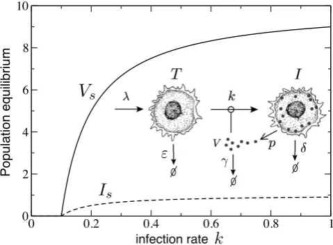
FIG. 4: Simple models and complex interactions. Second-order phase transition showing how the equilibrium values of the virus population (Vs, solid line) and infected cells (Is,
dashed line) diminish at decreasing the infection ratek. The inset displays a schematic diagram of the model, with the in-teractions between the susceptible cells (T) and viruses (V) (drawings by R. Sol´e). See Eqs. (13)-(15) for the mathemati-cal description.
B. Intrahost infection dynamics
When a model of cell-virus interactions is to be build, population biologists usually consider the number of in-dividuals in each two species (say X and Y for cells and virus, respectively) as the key variables. Interac-tion, growth and mortality parameters are then intro-duced and the main problem is how to properly express the functional relations associated to all these processes (Case 2000). The reactions required to represent this Lotka-Volterra type model (May 1973; Gotelli 1988) are represented schematically in the inset of Fig. 4. One could say that this is too simple to represent the true complexity of a natural virus-cell system, but the truth is that this toy model accounts for one particularly rel-evant property of these systems, namely the presence of cycles, which are a consequence of the internal dynamics of the system. Instead of being driven by some exter-nal driver, the nonlinearities of the model fully account for the emergence of oscillatory behaviour. This oscilla-tory regimes have been recently identified in mathemati-cal models incorporating further complexity in infection processes (Nurtayet al. 2018).
Consider now the problem of a minimal model of vi-ral infection (Fig. 4) where three variables are at least needed: the number of target cells (T), the number of infected cells (I) and the amount of viruses (V). This model has been studied in detail elsewhere (Perelson and Nelson 1999; Statfordet al. 2000; Perelson 2002; Nowak
this process generates infected cells, which produce virus particles at some rate p (the burst size). All the three populations decay with given rates (indicated asε, δ and
γ in the inset of Fig. 4).
The set of interactions also involves pairwise ’reac-tions’, but in this case viruses transform their host (turn-ing T cells into infected I cells) into a different type of ’particle’ and moreover they are produced by the in-fected cell populationI at a constant rate. Additionally, the model assumes a completely mixed system where en-counters between viruses and cells occur at random with homogeneous rates. This is of course another simplifica-tion: susceptible cells are usually strongly structure in space forming tissues, the model considers no evolution of the viral component, which of course is also a very strong assumption.
The following set of equations describes the basic dy-namics outlined in the inset of Fig. 4:
dT
dt = λ−εT−kV T (13) dI
dt = kV T −δI (14) dV
dt = pI−γ V. (15)
This model gives intuition concerning the potential outcomes of the infection dynamics. It has two alter-native equilibrium points (steady states), obtained from
dT /dt = dI/dt = dV /dt = 0. The first corresponds to the virus-free system, and is given by S0 = (λ/ε,0,0),
whereas the second equilibrium point provides the steady state S1 = (Ts, Is, Vs) where we have a steady infected
population
Is=
1
δ
1−εγδ
pk
(16)
and the equilibrium value for the virus population given by
Vs=
p δγ −
ε
k. (17)
The last expression gives a critical condition for the virus to persist: since we needVs>0 to meet this condition,
we havep/δγ > ε/k or, by rearranging terms, if
R0= pk
δγε>1. (18)
R0is known as the basic reproductive number,
represent-ing a threshold condition for infection success occurrrepresent-ing when R0 > 1. R0 thus defines the critical value for a
second-order transition, as shown in Fig. 4 by tuning the infection ratek.
This only one among many different models of virus-host interactions and in particular the role played by immune responses. Several monographs have explored diverse scenarios (Nowak and May 2000; Wodarz 2007;
Bocharov et al. 2018; see also Perelson and Weisbuch 1997 for a more physics-oriented view). Despite the po-tential richness and high-dimensional character of ex-tended models, it is often feasible to find the condi-tions for successful propagation by means of simple mod-els. This has also important consequences for defining the critical conditions for successful therapies (Perelson 2002).
C. Epidemic thresholds
Epidemiological models are diverse in their structure and complexity, depending on how many categories of in-dividuals are included and whether they are deterministic or incorporate stochastic components. The simplest pos-sible model is the susceptible-infected-susceptible (SIS) one, that only includes susceptible (S) and infected (I) individuals. This is a toy model, and some basic assump-tions are required. The first one being thatI+S =N, which means that, at some scale, the total population re-mains constant. Secondly, there is no heterogeneity and thus all interactions between individuals are weighted with exactly the same parameter values. In a well-mixed system, the rules outlined above can be described with two reactions associated to infection and recovery, given by:
I+S−→µ 2I, (19)
I−→α S. (20) It is easy to show that the equations describing our sys-tem are:
dI
dt =µIS−αI =− dS
dt (21)
and since the total populationI+S is conserved, using a normalized density of infected individualsρ=I/N, we have
dρ
dt =µρ(1−ρ)−αρ (22)
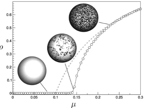
consistently with the previous result. We now have a one-variable model that can be solved analytically. This equation is actually the well-known logistic model with density-independent decay rate. This simple model is known to suffer a smooth transition asµdecreases below a given threshold (Fig. 5). Indeed, the mathematical pic-ture of this smooth continuous phase transition is given by the so called transcritical bifurcation (Strogatz 1994). Equation (22) can actually be re-written in a logistic-like form by definingρ∗= 1−α/µ,i.e.
dρ
dt =µρ(ρ
∗−ρ), (23)
Ifρ0that represents the initial condition, the solution of
this differential equation is:
ρ(t) = ρ
∗
1 +ρρ∗
0 −1
After long periods of time, i.e., in the limit ρ∞ =
limt→∞ρ(t) two solutions are possible, namely ρ∞ =ρ∗
whenµ > αandρ∞= 0 whenµ < α. The first point
in-volves a stable epidemic event that would infect a fraction (1−α/µ) of individuals of the population, whereas the second represents the extinction of the virus. The critical point µc =α separates the subcritical phase, where the
epidemics dies out from the supercritical phase, where the epidemics is self-maintained.
An important result from the previous model definition is that, at the supercritical phase, the initial growth of the epidemics is exponential. This can be shown by assuming that the current relative frequency of infected individuals is very small, i.e., ρ1. In this case, it is possible to make the approximation 1−ρ≈1 and thus the equation for epidemic spreading now becomes:
dρ
dt ≈α(R0−1)ρ, (25)
where we defineR0=µ/αas the basic reproductive
num-ber. Using this definition, an exponential growth is ob-tained
ρ(t) =ρ(0)eα(R0−1)t. (26)
which is positive (and epidemic spreading occurs) pro-vided that R0 > 1 and the epidemic would die out if
R0 < 1. R0 can also be seen as a the critical point at
which the system transitions from no epidemic to epi-demic success. Values of R0 are quite variable among
viruses. For example, it was estimated in the range 1.5 -2.5 for the Ebola virus. It ranges from 2 to 5 for the sex-ual transmission of HIV-1, while the measles virus, which is airborne transmitted, has R0 values ranging from 12
to 18. It is interesting to note that R0 involves several
components, including the infectivity of the pathogenµ, the recovery rate αand the population size N. There-fore, the behaviour of the critical point can be explored as a function of any of these three parameters,e.g.,µas shown in Fig. 5.
This very basic SIS model can be improved by adding specific spatial structure: hosts live in a lattice and the probabilities of transmission depend on the physical dis-tances between individuals in the lattice. Obviously, this system makes computations slightly more complicated, but the conclusion is that a critical R0 can still be
re-covered as a function of the rate arrival of infected indi-viduals into the population,β, and the rate of recovery,
α(Anderson and May 1998): R0 =β/α, which still
de-fines a second-order phase transition. The exact location of the transition point has moved and the shape of the curve on the right hand side (Fig. 5) is slightly different, but the phenomenon itself remains preserved.
D. Large-scale pandemics on networks
In the previous section we have considered in certain detail the very simple SIS model of epidemic spreading
FIG. 5: Epidemic spreading as a continuous transition (dashed line). Here we use α = 0.1 and plot the station-ary fraction of infected individuals (ρ) against the infection rate, µ. For comparison, we also display the same plot for a spatially extended system on a two-dimensional 100×100 square lattice. Here, infected and susceptible sites are shown as black and white patches. The spatial effects make more difficult the propagation of the epidemics and thus the criti-cal point predicted by the mean field theory is found at higher values ofµ.
that occurs in a well mixed (mean field) context. Simi-lar results would be found by assuming that individuals interact at random with a given probability. However, the networks of interactions among humans can depart from the mean field approach. Similarly, transportation networks connecting humans on large scales strongly de-part from these simplified pictures (Pastor-Satorras and Vespignani 2001; Lloyd and May 2001; Brockman and Helbing 2013; Pastor-Satorras et al. 2015; Barab´asi 2016).
If we look at the probability P(k) of a node (e.g., an airport) being connected to k other nodes, they follow heavy-tailed distributions described as scaling laws, i.e.
P(k)∼k−γ, whereγ is known as the scaling exponent.
Here we will explore the problem of epidemic spreading in scale-free networks by means of a SIS model. Each node in the graph of interactions represents and individual and each link a potential transmission event. The average density of infected individuals ρ(t) (prevalence) at the mean-field level is
dρ(t)
dt =µhkiρ(t) [1−ρ(t)]−αρ(t), (27)
whereµis the infectivity of the virus andhkithe average degree of the graph (i.e. the number of connections per node). As we can see, we have just recovered the mean field equation for the SIS model, given by Eq. (22).
By defining an effective spreading rate λ = µ/α, we can write:
dρ(t)
a
b
c
d
FIG. 6: Lack of eradication thresholds in epidemic models on scale-free networks. Large-scale transportation networks, such as the international web of airports (a) display highly heterogeneous connectivity distributions (picture after Dirk Brokman). (b) Mean field model prediction displaying a phase transition (in a SIS mode, continuous line) is compared with the one shown for a scale-free network (dashed line). When dealing with disease transmission networks among humans, which also display scale-free structure (c), protecting the hubs can effectively make the web homogeneous (d) thus recovering the standard, second-order transition found in homogeneous graphs(d). Insets c-d adapted from Barab´asi (2016).
The benefit of this mean-field equation stems from the fact that density correlations are ignored. On random graphs and related graphs, one can assume thatk' hki. It is easy to demonstrate that a non-zero epidemic thresh-old exists atλc=hki−1 such that
ρ = 0 ifλ < λc, (29)
ρ ∼ 1− 1
hki ifλ≥λc. (30)
So far, everything seems pretty much the same, but a crucial property of scale-free networks changes every-thing (Pastor-Satorras and Vespignani 2001; Lloyd and May 2001; Dezs¨o and Barab´asi 2001; Barab´asi 2016). The fluctuations k2 in scale-free networks diverge for
any value of the critical exponent 2 < γ < 3 and thus highly connected nodes are statistically significant: the mean field approximation breaks down. In order to take
into account these fluctuations, the relative densityρk(t)
of infected nodes with given connectivitykmust be taken into account. The mean-field equations can thus be writ-ten as
dρk(t)
dt =λk[1−ρk(t)] Θ(ρ(t))−ρk(t) (31)
fork= 1, ...N. A new term Θ(ρ(t)) indicates the proba-bility that any given link points to an infected node. The probability that a link points to a node withk links is proportional to kP(k). A randomly chosen link is thus more likely to be connected to an infected node with high connectivity, yielding
Θ(ρ(t)) = P
kkP(k)ρk(t)
P
kkP(k)
, (32)
dρk(t)/dt= 0, and hence
ρk =
λkΘ
1 +λkΘ (33)
and the following relation follows:
Θ = 1
hki
X
k
kP(k) λkΘ
1 +λkΘ, (34)
where Θ is now a function ofλalone.
The solution Θ = 0 is always satisfying the previous equation. A non-zero stationary prevalence (ρk 6= 0) is
obtained when the right hand and the left hand sides of Eq. (34), expressed as function of Θ, cross in the interval 0 < Θ≤ 1 allowing a nontrivial solution. It is easy to realize that this corresponds to the inequality
d dΘ
1
hki X
k
kP(k) λkΘ 1 +λkΘ
!
Θ=0
≥1 (35)
being satisfied, defining the critical epidemic threshold by:
P
kkP(k)λck
hki =
k2
hki λc= 1, (36)
or rewritten as
λc= hki
hk2i, (37)
which is nothing but the inverse of the coefficient of vari-ation of the network’s degree (CV, Anderson and May 1991). This result means that in scale-free networks with
γ ∈ (2,3) λc = 0 (see dashed line in Fig. 6b) and thus
for any value of λthe infection can pervade the system with a finite prevalence (Pastor-Satorras and Vespignani 2001). For small λ it is possible to solve explicitly the previous equation and calculate the prevalence in the en-demic state as follows:
ρ=X
k
P(k)ρk. (38)
In the particular case of the Barab´asi-Albert network with γ = 3, we haveρ∼exp(−C/λ) whereC is a con-stant.
The absence of any epidemic threshold in this network can be understood by noticing that in heterogeneous sys-temsR0contains a correction term linearly dependent on
the standard deviation of the connectivity distribution. In scale-free networks the divergence of the connectivity fluctuations always leads to anR0>1 at any rateλ. This
ensures that epidemics always have a finite probability to survive indefinitely. This of course makes more difficult to properly exploit a propagation threshold and define containment strategies. However, it is possible to ”cure” the hubs (by immunizing them) and generate an effective threshold (Dezso and Barab´asi 2002; see also Kitsaket al.
2010; Wanget al. 2016; see also Hufnagel et al. 2004). The key idea here is that, once these highly connected nodes are protected from infection, the remaining graph is not fat-tailed anymore, as shown by the inset graph in Fig. 6d. The presence or absence of epidemic thresh-olds in the real world has thus considerable implications, both in the context of disease spreading and the propa-gation of computer viruses (see Sol´e and Elena 2019 and references therein).
III. THE EVOLUTIONARY DIMENSION: MULTIPARTITE VIRUSES AND MUTUALISM
The previous examples illustrate how simple dynami-cal models can display marked changes in the behavior of a diverse range of problems in virology. Except for the self-assembly problem, all these case studies share a uni-fying feature: in a way or another, the transition requires achieving a critical threshold level of infection beyond which propagation occurs. There is, however, another layer of complexity beyond these two-phase systems that has to do with the nature itself of ecological interactions and their impact on virus evolution. Crossing thresh-olds in these cases has consequences for the presence or absence of cooperative interactions among different viral components.
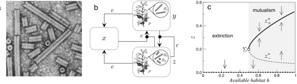
Transitions between different kinds of population level dynamics, such as competition versus mutualism or par-asitism, are particularly important for evolutionary biol-ogy. What kind of transitions can be found in models of virus dynamics? A very interesting example is given by a particular class of RNA viruses known asmultipartite viruses(Iranzo and Manrubia 2012; Sicard et al. 2016, 2019; Luc´ıa-Sanzet al. 2018). In a multipartite virus, no single viral particle contains all the genomic segments, which appears segregated in two or more particles. As a consequence, the information required for a full infection cycle is not linked into a single molecule but distributed. An example of multipartite virus (Fig. 7a) is tobacco rattle virus (TRV), which infects, along with tobacco, many other plant species. It consists of two particles, a long and a short one. The first contains the RN A1
segment encoding for the replicase, while the second par-ticles encapsulatesRN A2 segment that encodes for the
coat protein. As a consequence, the long particle can in-fect and trigger the disease on its own, but the RN A1
tran-a
b
R1 R2
P R1
P
x
y
z
c
e
c
e mutualism
extinction
z⇤ z+⇤
⌃
c
FIG. 7: Multipartite viruses include two or more genomic segments, encapsidated independently, and all required to complete the full life cycle of the virus. An example is tobacco rattle virus TRV, shown in (a) where we can appreciate the presence of two kinds of particles (image by John Antoniw). A simple metapopulation model with a simple set of transition rules (b) can help to explore the population and evolutionary traits of multipartite viruses. In a simple model of multipartite virus dynamics (Nee 2000) the previous set of rules led to a sharp transition phenomenon (c) where the abundance of plants carrying the two components of the multipartite virus are indicated againsth.
sitions between states, as described in Fig. 7b. Here a given habitat is considered, which can be visualized as a grid of patches, as usual in many models of metapopula-tion dynamics (Mollanen and Hanski 1998; Hanski 1999). Patches can be empty, occupied by a plant carrying only
RN A1or plants carrying the two components of the
mul-tipartite virus. These populations (normalized) are indi-cated asx, y, zrespectively. A fraction 0≤h≤1 of this habitat is occupied.
Two main events are considered here: colonization, at a given ratecand extinction, at a ratee. Both are prob-abilities and thus 0≤c, e≤1. The basic model defining the dynamics of each component is given by (Nee 2000):
dx
dt = ey+ez−czx, (39) dy
dt = −ey+czx−czy, (40) dz
dt = −ez+czy, (41)
with a normalization condition defined by:
h=x+y+z. (42) This constraint allows to reduce our three-equation model to a two-dimensional system,i. e.
dy
dt = −ey+cz(h−y−z)−czy, (43) dz
dt = −ez+czy. (44)
The equilibrium points obtained fromdy/dt=dz/dt= 0, are (after some simple algebra)
x∗ = h−y∗−z∗, (45)
y∗ = e
c, (46)
z±∗ = 1 2 h−
2e c ±
r
h2−4eh
c
!
. (47)
A domain involving three possible equilibrium points (two of them stable) is given by the condition
h2−4eh
c ≥0 (48)
i. e. the argument within the square root needs to be positive. This will occur provided that
h > hc=
4e
c . (49)
This is illustrated in the bifurcation diagram in Fig. 7c, where the possible equilibrium values of z are plot-ted against the available population sizeh. The discon-tinuous jump separating the phases of mutualism and extinction is given by the so-called saddle-node bifurca-tion, which often arises in systems with positive feedbacks such as facilitating or cooperation. The diagram thus indicates that a minimal accessible number of individ-uals (plants in our metapopulation context) is required to allow for the propagation of the multipartite viruses. This is indicated by the extinction phase (left), separated by a mutualistic, persistence phase (gray domain). The positive solution starts at a value z∗ = Σ defining the
minimal (critical) population size. This result is related to those found within the context of extinction thresh-olds in metapopulation models due to habitat loss and fragmentation including continuous (Bascompte and Sol´e 1996) and first-order (Sardany´eset al. 2019) transitions. It thus connects the problem of reduced habitat and the persistence of viral associations requiring higher-order in-teractions (such as mutualism).
are affected (among other things) by the multiplicity of the infection (Lucia-Sanz and Manrubia 2017). The full analysis of these models reveal a rich phase space where diverse phases include competition, mutualism and com-mensalism.
IV. INFORMATION AND DIVERSITY TRANSITIONS
In this section we expand our previous case studies of phase transitions with three more examples. These cases are not related to transitions at different levels of virus organisation, as we have discussed so far, but with another type of phenomena: phase transitions involving changes in information and genetic diversity. The first example is the well known phenomenon of the meltdown of genetic information at increasing mutation rates, with viral populations entering into the so-called error catas-trophe regime. This is a nice example of second-order phase transition. The second example has to do with the dual role of homologous recombination in the rescue of mutationally compromised populations if recombination is at some critical value, or driving them to extinction if recombination is far too high. Interestingly, the first situation corresponds to a second-order phase transition, while the second situation corresponds to a first-order one. The third example deals with the role of within-host HIV-1 diversity in the progression towards AIDS, which is also a second-order phase transition.
A. The error catastrophe
Because of their intrinsic simplicity and their strong dependence upon the host molecular machinery to com-plete their cellular infection cycle, viruses are unique dy-namical systems. One particularly important trait of RNA viruses is their high mutation rates, much higher than any other rates exhibited by cellular systems and a consequence of the lack of repair mechanisms associ-ated to their RNA-dependent RNA polymerases (the in-set in Fig. 8 shows the structure of hepatitis C virus repli-case). This enzyme catalyses the replication of RNA tem-plates producing new RNAs and mutation rates per nu-cleotide and replication cycle are in the range 10−4
−10−5
(Sanju´an et al. 2010). Recent research has also deter-mined mutation rates of about 10−3 per base per cell
in the revers transcriptase of HIV-1 (an RNA-dependent DNA polymerase) in peripheral blood mononuclear cells (Cuevas et al. 2015). In DNA-based systems, such as the cellular hosts, the process of DNA polymerization is usually associated to a proofreading and highly efficient and redundant repair mechanisms that effectively reduces mutation rates to a range 10−8−10−11 ensuring a
con-trolled replication cycle (Drakeet al. 1998). Since high mutation carries a burden of genetic errors, this implies
⌫
µ
viroids
RNA viruses
ssDNA!
viruses
dsDNA!
viruses Bacteria
Lower !
eukaryotes
Higher!
eukaryotes
µ⇠⌫ 1
a b
FIG. 8: Scaling law in the per-site mutation rate (µ) versus genome size (ν), shown in log-log scale. The plot includes chosen examples of RNA viruses, which lack error-repairing mechanisms during replication (the inset displays the struc-ture of hepatitis C virus RNA replicase (image obtained from the wikipedia)). Larger genomes are represented by both single-stranded and double-stranded RNA viruses and DNA viruses, bacteria and a few eukaryotes (adapted from Gagoet al. 2009). The continuous line is used to highlight the inverse law linking mutation rateµ and genome length ν predicted by the error threshold theory.
that many resulting viral genomes can contain deleteri-ous changes leading to non-viable viral particles.
Mutation is a crucial component of evolution, as ge-netic variability is the fuel on which natural selection operates to adapt populations to their environment. In this sense, an error-prone polymerase can be seen as use-ful to keep pace with the always changing environmental conditions in which RNA viruses live (Domingo 2000). However, keeping in mind that mutation is a random pro-cess independent on the value that mutations may have in the future generations, mutation itself is a double-edge sword: too many mutations per genome may simply drive fitness levels to such a low values that would not be com-patible anymore with a successful replication. Therefore, mutation rates, as any other trait, have evolved and have been optimized for the lifestyle of RNA viruses: just high enough but not more (Elena and Sanju´an 2005). For RNA viruses, a heterogeneous population results in a so-called viral quasispecies (Eigen 1971; Eigen et al. 1987; Schuster 1994; Domingo and Holland 1994; Domingoet al. 1995; Domingo et al. 2012). A viral mutant swarm can be seen as a group of genomes dominated by a master sequence of high fitness that may, or may not, coincide with the average sequence of the population, the consen-sus sequence.
0000
1000 0010
0011
0111 0110
1111
1100 0001
0101 0100
1010 1011
1001
1101 1110
1011
0000
1000 0010
0011
0111 0110
1111
1100 0001
0101 0100
1010 1011
1001
1101 1110
1011
0000
1000 0010
0011
0111 0110
1111
1100 0001
0101 0100
1010 1011
1001
1101 1110
1011
a
b
c
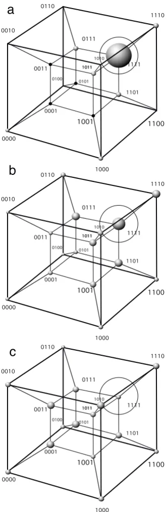
FIG. 9: The error catastrophe on a four-dimensional hy-percube. Three occupation patterns for 4-bit strings are shown: strings 1111 have a large fitness fm, whereas all
s1s2s3s4 6= 1111 (si∈ {0,1}) have the same, smaller fitnessf.
Strings replicate with a mutation rateµper bit. (a) Starting with all 1111 strings, very smallµ leads to a large majority of strings located at 1111. (b) Larger mutation generates a more disperse mutant cloud still surrounding the node 1111 (b). (c) A mutation rate close to its critical value allows to preserve a cloud of strings while generating much more diver-sity and keeping the information of sequence 1111. Beyond the threshold, the population experiences pure genetic drift and the master sequence is not found at all.
within the context of the virus infection and pathogen-esis, that includes the host responses tied to immunity but also others such as tissue specificity or resistance to drugs (Andino and Domingo 2015; Domingoet al. 2012; Lauring and Andino 2010; Holmes 2010).
One particularly unexpected consequence of the qua-sispecies nature of viral populations is deeply connected to the informational nature of RNA viruses. This is known as the error catastrophe problem (Eigen 1971; Eigenet al. 1987; Schuster 1994; Domingo and Holland 1994) and is tightly related with second-order phase tran-sitions. It was originally defined within the context of an abstract population of mutating molecular replicators competing for limited resources. More precisely, Eigen and Schuster considered a large population of genomes where each sequence could replicate at some fix rate. Replication rate will be sequence-dependent and the re-lation between sequence and growth rate should be ex-pected to be complex. Additionally, it is assumed that every time a string replicates, mutations can occur at a given rateµ.
Eigen (1971) predicted that there is a critical mutation rate,µc, that decays asµc∼1/ν beyond which no
Dar-winian selection can occur, and thus no viable sequences would be observable for mutations higher thanµ > µc.
In that case, random drift would be observed. Instead, below the threshold, information can be maintained in stable ways. Experimental data confirms this inverse re-lationship. and thus mutation rates decrease as an in-verse power law of genome length (Fig. 8). RNA viruses exhibit the highest rates, orders of magnitude larger than DNA viruses. At this point, two questions emerge: what is the origin of such relationship? And what are the limits (if any) of mutation rates in RNA viruses?
Eigen-Schuster quasispecies model (Eigen 1971) con-siders a set of populations {xi} representing the
abun-dance of different genomes, changing in time by the fol-lowing set of dynamical equations:
dxi
dt =
n
X
j=1
fjµ(j→i)xj−Φ(x, t)xi, (50)
where xi indicates the fraction of the population
asso-ciated to the i−th mutant genome equipped with a M -letter alphabet (here i = 1, ...n, wheren = Mν is very large,νbeing the length of the genome) so that a normal-ization condition applies, namely: Pnj=1xj= 1. Here fj
is the growth rate of the j-th mutant, µ(j → i) is the probability of having a mutation from sequencej to se-quence i and Φ(x)c is the average fitness associated to
cΦ(x) is usually termed as the dilution outflow, which ensures a
constant population (Pn
i=1xi= constant andPni=1x˙i= 0) also
the population vectorx= (x1, ...xn),i.e.,
Φ(x, t) =
n
X
j=1
fjxj n
X
i=1
µ(j →i) !
=
n
X
j=1
fjxj=hfi.
(51) This model can sometimes be treated analytically under a number of well defined set of conditions, showing that the population structure corresponds to a cloud of sequences (Eigen 1971; Eigenet al. 1988, 1989; Schuster 1994).
In this section we consider a specific case that will il-lustrate how mutation can sharply limit the length of genomes and thus the amount of information stored in a quasispecies.Many possible extensions are not considered here, such as the introduction of spatial degrees of free-dom (Altmeyer et al 2001; Pastor-Satorras and Sol´e 2001; Aguirre and Manrubia 2008; Sardanyes and Elena 2011), secondary RNA structure (Stitch et al. 2007) or more complex fitness landscapes (Saakian et al 2006; Saakian 2018).
The problem considered here can be mapped into a high-dimensional sequence hyper-cube (Fig. 9) , where each string is a digital genome, connected to nearest neighbors in the cube that differ by one bit (single muta-tion), considering binary genomes i.e. M = 2. Without loss of generality, the general model described above can be collapsed into only two fitness classes, namelyfm for
the master and f for any other sequence of the mutant spectrum (i.e., f1 =f2 =...=fn =f) where nis very
large (n 1). Hereafter it is assumed that fm > f,
i.e., the master sequence replicates more efficiently than any other sequence (Swetina and Schuster 1982). As-suming that i.e., µ(i→j) = µ, we can split our system of equations into two sets: the master sequence and the mutant sequences. The system presented below is only a simplified approximation to the space connecting dif-ferent genomes. A more accurate picture is provided by Fig. 9(b): from a given populationxj, mutation will not
lead back to the master sequence or will be difficult to occur. In this case, we will havexm+x= 1 where we
usex=Pjxj. For the master sequence we get:
dxm
dt =fm(1−µ)xm+
n
X
j=1
fj
µ
nxj−xmΦ(t), (52)
whereas the set of equations for the mutant sequences reads:
dxi
dt = fmµ
n xm+
n
X
j=1
fj
µ
nxj−xiΦ(t). (53)
It is easy to show, after some algebra, that the first equa-tion can be simplified to
dxm
dt =≈fm(1−µ)xm−xmΦ(t), (54)
where we have used µ/n1. For the equation
describ-ing the mutant class, we have:
dxi
dt = fmµ
n xm+f(1−µ)xi+
n
X
j6=i
f µ
n xj−xiΦ(t). (55)
Since the ultimate goal is to describe the dynamics of all these populations together, so we made the sum over all possible mutant genomes,i.e.,
n
X
i=1
dxi
dt =
n
X
i=1
fmµ
n xm+
n
X
i=1
f(1−µ)xi
+
n
X
i=1
f µ n
n
X
j6=i
xj
−
n
X
i=1
xiΦ(t)
=µfmxm+f(1−µ)x+f µ(x−xi)−xΦ(t). (56)
Given the homogeneous mutation rates, a stationary dis-tribution will lead toxi≈x/nand thus the
approxima-tionx−xi≈xis guaranteed, leading to
dx
dt ≈µfmxm+f x−xΦ(t), (57)
and as a result of these approximations, the two-compartment model (Fig. 9(a)) can be collapsed into a one-dimensional system (Swetina and Schuster 1982):
dxm
dt = fm(1−µ)xm−xmΦ(xm, x), (58) dx
dt = fmµ xm+f x−xΦ(xm, x). (59)
As we did above for the replicator model, the condition
xm+x= 1 leads to Φ(t) =hfi=fmxm+f x. Using this
function, and sincex= 1−xm, it can be obtained after
some algebra an equation for the master sequence:
dxm
dt =xm[(1−xm)(fm−f)−µfm]. (60)
Two alternative equilibria are possible. The first one beingxm= 0, that corresponds to the extinction of the
master sequence and the full dominance of the pool of mutants, and a nontrivial equilibrium
xm= 1− µfm
fm−f, (61)
allowing the coexistence of both master and mutant se-quences. The later solution will be positive (and the master sequence will be present) provided thatxm > 0
and this will occur if the mutation rate is lower than the critical value:
µ < µc= 1−f /fm. (62)