Evaluation of Lower Bounding Methods of Dynamic
Time Warping (DTW)
Happy Nath
Department of CSE, NIT Silchar Cachar,India
Ujwala Baruah
Department of CSE, NIT Silchar Cachar,India
ABSTRACT
This paper presents a brief review on the lower bounding(LB) methods applied on Dynamic Time Warping(DTW) till now. Apart from providing a survey on the methods, an attempt has been made to compare these methods in terms of constraints involved with these methods. Some Lower Bounding (LB) methods have better pruning power than others, some are better in terms of running time and also there are some which do introduce greater number of false dismissals than others. This work will help researchers in selecting a suitable lower bounding method for their application. The authors hope that this work will provide a scope of evaluating Lower bounding distances of DTW in the area of speech recognition and verification in general and will also help identify research topic and application in this area.
Keywords
DTW, Lower Bound, Indexing, Data Mining.
1.
INTRODUCTION
Dynamic Time Warping (DTW) is a template matching algorithm in pattern recognition ,which can align sequences which vary in time or speed. It was introduced and explored in speech recognition for the first time by sakoe and chiba[15]. In data mining it was introduced in 1994[ 14].
The alignment produced by DTW is non-linear ,which is different from the linear alignment produced by other distance measure like Euclidean distance.
Fig.1 alignment produced by Euclidean distance and DTW distance
The basic idea is to match a test input represented by a multi-dimensional feature vector
T
(
t
1,
t
2,....
t
J)
with a reference templateR
(
r
1,
r
2,...
r
I)
. At first the cost matrix is formed in which the cost of each index(i,j) in that matrix is the Euclidean distance between thei
thandj
thpoint respectively on the two sequence. After that the warping matrix is formed based on the dynamic programming .Then optimal path is formed by trace backing and minimized score is returned. The dynamic programming used is –))
1
,
1
(
),
1
,
(
),
,
1
(
min(
)
,
(
)
,
(
i
j
d
T
R
f
i
j
f
i
j
f
i
j
f
i jWhere
d
(
T
i,R
j)
is the distance between points(
T
i,R
j)
which is generally Euclidean distance though other distance measures are also used.Fig.2. Warping path between two sequence T and R
In order to search for similarity with an input query, generally all the sequences in the database need to be read and also DTW distance for all of them must be computed to get the most similar or a set of similar sequences . It is highly expensive in terms of I/O and CPU. So, we need some procedure by which the DTW computation is not done for the sequences which cannot probably be the best match with the input sequence .Indexing and lower bounding distance measure is used to solve the problem. If there is an indexing scheme ,then for retrieving
time
time
T
R
similar sequence, all the sequences are not necessarily to be read . And if there is a lower bounding measure ,then some sequences from the database are pruned off before their full DTW computation. Indexing together with lower bounding distance measure provides great advantage.
Some conditions that a similarity function must have in order to allow easy indexing. These are-
)
,
(
)
,
(
P
Q
D
Q
P
D
Symmetry0
)
,
(
P
P
D
Self-Similarity0
)
,
(
P
Q
D
Positivity)
,
(
)
,
(
)
,
(
P
Q
D
P
R
D
Q
R
D
TriangularInequality
The property “triangular inequality” creates some problem sometime in indexing. When the similarity measure does not follow “triangular inequality” property , then false dismissal occurs [ 1 ]. So, in DTW exact indexing is a problem. There are two types of indexing in DTW- Exact indexing and approximate indexing[1,3]. In exact indexing ,the best match is returned according to DTW. In approximate indexing, not necessarily best match, but good matches are returned. So ,in the latter case, i.e., in case of approximate indexing ,when best match is not returned and instead good match is returned, obviously false dismissal occurs . Although, since false dismissal is a major concern in similarity search indexing, yi et al[1] already explained the fact that only in sequential scanning ,false dismissal does not happen ,in the rest all indexing it occurs more or less since they assume triangular inequality.
Lower bounding distance is a distance which needs lower computation time than the actual DTW distance between the two sequences. In lower bounding ,one first computes the lower bound of the DTW distance between the two time series. A best-so-far distance is set to infinity. If this lower bound is less than the best-so-far distance then DTW calculation is done otherwise the time series is pruned off since it could not be the best match. If this DTW distance is less than best_so_far distance , then best_so_far distance is changed to the value of the DTW distance.
Lower bounding measure must have the following properties- 1) It must be fast to compute. Obviously, if lower
bounding measure takes time more than that of actual DTW time, then it is of less use. So, it is expected that
LB
dist(
R
,
T
)
DTW
dist(
R
,
T
)
,wheredist
LB
is the lower bound distance .From here it is obvious that ifDTW
dist(
R
,
T
)
,then
)
,
(
R
T
LB
dist [yi et al]. So, no false dismissal.2) It must be a tighter lower bound.
Tightness of a lower bounding measure can be defined as the ratio of lower bound distance to the actual DTW distance. The ratio is in the range[0,1].The higher the ratio, the tighter is the bound. Pruning ratio is the number of DTW computation while using lower bounding measure to that without using lower bounding measure. Smaller the ratio ,better the pruning power. High dimension of the series also is a problem for indexing schemes. Therefore ,almost all the lower bounding measures employed some dimensionality reduction techniques.
2.RELATED
WORK
2.1
Lower bound by Yi et al 1998,[1]
Yi et al introduced the lower bounding technique in DTW. They have given two techniques in a pipelined fashion to speedup DTW .The first technique is the Fast Map[4 ] technique to index sequence with DTW distance. The second technique is the lower bounding one. Fast Map technique maps sequences in K-d Euclidean space so that distance between them are approximately preserved. After that any spatial methods(e.g., R-tree[7]) are used to organize and search for the queries. The time is constant O(N) with respect to the input sequences N. At the filtering step of indexing, two sequences are compared in terms of k-d Euclidean distance only and the irrelevant distances are filtered out. In this process if any non-qualifying sequence is included, then it is removed at post processing step. The lower bounding measure is the sum of the difference between the maximum of the query sequence and the elements in the data sequence that are greater than that maximum also those which are smaller than the minimum of the query sequence. Figure 6 diagrammatically depicts the lower bound. This lower bound is popularly known as LB_Yi.
2.2
Lower bound by Kim et al 2001,[2]
Kim et al. extracted 4 types of features from the sequences. These four features are first(S), last(S), greatest(S), smallest(S), where S is a sequence. Since, while warping the sequence is stretched, so these 4 features do not change after time warping the sequence.
D
twlbis the lower bound distance which is the maximum of difference between first of the two sequences, last of the two sequences, greatest of two sequences and smallest of two sequences. Figure 7 can give a well explanation.The 4 features extracted from each sequence are used for indexing purpose where
D
twlbis used as a distance function, since it consistently satisfies triangular inequality. For organizing the sequence in the space any multidimensional index (such as R-tree, X-tree) is used.lb tw
D
is used as the lower bounding distance. This lower bound is popularly known as LB_Kim.2.3
Lower bound by Keogh et al,2002[4]
This lower bounding technique is termed as LB_Keogh, which is an exact lower bounding .Piecewise Aggregate Approximation (PAA) (Keogh et al. 2000; Yi and Faloutsos2000) is used for dimensionality reduction technique which they term as Keogh_PAA. Figure 8 diagrammatically depicts PAA.
The envelop of the query sequence is first developed using the warping windows(Sakoe Chiba band[15] and Itakura parallelogram[8]). If
W
k
(
i
,
j
)
kis the warping path and ‘r’ is the allowed range of the warping window thenr
j
i
r
j
The envelop of the sequence is calculated by the formulas-);
:
max(
i r i ri
q
q
U
)
:
min(
i r i ri
q
q
in the data sequence and also that between lower envelop of query sequence and elements in the data sequence.
[image:3.595.66.291.132.369.2]Authors Showed that the lower bound which uses Itakura Parallelogram is tighter than that which uses Sakoe Chiba band .
Fig. 3. Lower bound LB_Keogh .U is upper bound, L is lower bound and Q is query
2.4
Lower bound by Sakurai et al,2005[5]
Authors term this lower bound as FTW(Fast search method for Time Warping). At first, the time series is segmented and then similarity distance is calculated between two segmented time series. The algorithm works for segments of unequal length also. Each segment is associated and denoted by corresponding range and time interval. Each range again is associated with a maximum and a minimum value. Two new algorithms are used which are Early Stopping and Refinement. Early stopping is for restricting the scope of evaluating distance for the grid cells which does not satisfy a particular criteria. The criteria is that a current_best distanced
cb is maintained for the query sequence. When a similar sequence is found which gives distance smaller thand
cb,thend
cb is updated to the new distance. Refinement is used because sometimes as the segment granularity increases, distance also increases. So, that distance may sometimes be found greater thand
cb which should not be there in the answer set. Therefore, Refinement is used to check the distance by gradually increasing the granularity.Sequential indexing structure is used here so as to ensure that no false dismissal occurs[1].Unlike others which uses some index structure other than sequential, no cost is not required constructing the index structure .For efficiency K-nearest neighbor search algorithm is used.
Distance is calculated between segments of the sequence of a two ranges. The distance between the lower value of the segmented range to the upper value of another segmented range is returned as the lower bounding distance i.e., distance between two closest points and this distance is 0 if the two intersect.
Here ,for calculating lower bound distance , there is no restrictions on the warping window. Warping window may or may not be used. But it works better with large warping width or without any warping width constraint . FTW can give it’s best as data size or sequence length increases.
Fig. 4. Segmented time series[5]
2.5
Lower bound by Zhu et al,2003[6]
[image:3.595.308.474.132.232.2]The DTW used here is rather Local DTW(LDTW) .In LDTW,each sequence after stretching to the same distance compared point by point locally with some constraint k such that |i-j|≤k ,where i and j are the indices of a point in the warping path. The width of the warping path is
n k 1
2 (Sakoe-chiba band), where n is the length of the stretched sequence. The envelop of the query sequence is used and the distance between that envelop and data sequence is used as the lower bounding distance. The main contribution in this paper by Zhu et al is the container invariant transformation of the envelop which guarantees no false dismissal. As in general ,the transformation of the envelop is done for the dimensionality reduction purpose. A transformation is container invariant when for all the sequences of length n , the transformation of the envelop covers the transformation of the time series sequence. In special case, the transform of the sequence becomes equal with the transform of the envelop. A modification of Piecewise Aggregate Approximation (PAA) is used as dimensionality reduction technique although other techniques can also be used. In PAA ,the n dimensional sequence is reduced in dimension N by taking averages in N consecutive equal sized frames. Here a modifies PAA is used where each piece is the average of the upper or lower envelope during that time period.
This lower bounding technique produces fewer false dismissal.
2.6
Lower bound LB_Improved by
Lemire,2009 [10]
This is a modification over LB_Keogh. This lower bound is a two pass process and each process in turn is computation of LB_Keogh itself. PAA is used for dimensionality reduction purpose. LB_Improved is a two phase process. The first phase is the LB_Keogh itself. If candidate is not pruned out in the first phase, then the second phase is applied, otherwise not. At first phase, envelop is developed for the query sequence. Compare candidate sequence with this envelop .The result is LB_Keogh. In the second phase, project candidate on the envelop .Now compute envelop of the projection. Now compare this envelop with the query sequence. The result is LB_Improved. Then projection of the stored sequence is done on the query sequence. The projection of a stored sequence on the query sequence is the closest point of the stored sequence to the envelop( if it is U
L
Q
L
U
outside the envelop) and if it is inside the envelop then it is exactly that point. The lower bounding measure is now
)) , ( , ( _ ) , ( _ ) , (
_improved x y LB Keogh x y LB Keogh y H x y
LB
2.7
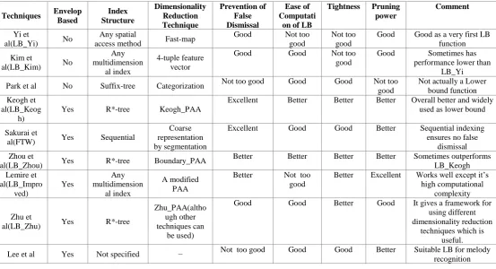
Lower bound by Lee et al,2005 [12 ]
Any appropriate indexing scheme can be used. The bounding envelop used here is for the type “anchored beginning, free end” with slopes 0.5 and 2 of the bounding lines.
Two types of measures they have used for lower bounding- a) Partition based method : Each candidate sequence is
partitioned into k number of subsequences starting from half of the length of query sequence to double of its length( since slopes are 0.5 and 2).
b) Correlation and approximate lower bounding functions: The margins of the bounding envelop is based on the standard deviation of the warping window at every index of the candidate song. At first, for each candidate sequence the correlation coefficient between the query and the k subsequence is calculated, the segment with highest correlation coefficient is kept. After that the lower bounding function is used. By adjusting the multiplying constant, we can have tighter or looser bounding function. The lower bounding function is approximate and cannot guarantee no false dismissal.
Fig.5. feasible warping reagion for music retrieval[12]
2.8
Lower bound by Park et al,2000.[11]
Park et al uses suffix tree as the index structure and two lower bound distance .This method guarantees no false dismissal since the suffix tree does not assume any distance function. But the time complexity is quadratic with the input sequences which is equivalent to raw DTW time complexity. In [4] Keogh et al explained that lower bound by Park et al gives bad result. Therefore this function is least regarded as the lower bounding function.2.9
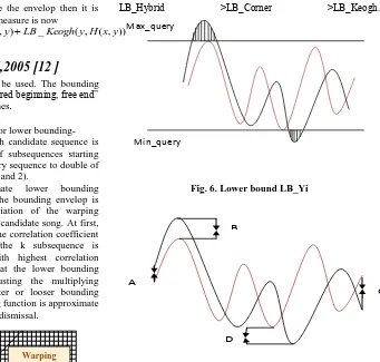
Lower bound by Zhou et al,2007.[9]
It is a boundary based lower bounding technique. It uses PAA for dimensionality reduction. Particularly a modification of Zhu_PAA which they term as Boundary_PAA. There is a set of boundaries and every warping path must pass through the boundary and any two boundaries cannot overlap. At each boundary we will get a lower bound and the summation of all those lower bounds collected serves as the lower bound distance for the DTW distance between the two sequences.
Three types of boundaries are defined Corner, Hybrid, and Stair. Boundaries are shown in Fig. 2 This also works on warping window. It has been shown that tightness of LB_Correr and LB_Hybrid outperform LB_Keogh. Considering tightness,
LB_Hybrid ˃LB_Corner ˃LB_Keogh.
Max_query
[image:4.595.200.541.70.395.2]Min_query
Fig. 6. Lower bound LB_Yi
A
B
C
D
Fig.7. Lower bound by Kim et al
3
COMPARISON
The comparison of the tightness and pruning power of the lower bounds LB_Keogh, LB_Kim and LB_Yi can be found from [3]. Diagrammatically it shows the comparisons. With respect to tightness LB_Keogh > LB_Yi >LB_Kim. With respect to pruning power LB_Keogh>LB_Yi >LB_Kim. In [10] , a good comparison of LB_Keogh, LB_Improved and LB_Zhu in terms of pruning power is there that can be explained with LB_Improved > LB_Keogh > LB_Zhu. The ease of computation of Lower Bound column has been created based on the various facts such as some lower bounds are very complex to compute and some are easier with respect to time e.g., LB_Improved is complex in this regard since it first computes the LB_Keogh for the sequence and after that it computes the LB_Improved. In [13] ,Comparisons of LB_Keogh, LB_improved and FTW can be found . Here , it has been shown that LB_Improved is complex despite of it’s better pruning power and FTW works very well with larger warping window. In [6], Comparison between LB_Keogh and LB_Zhu in terms of tightness is there. The prevention of false dismissal column is based on various facts like whether the indexing technique is exact or approximate. If it is exact ,then it will produce the same result as sequential indexing and if it is approximate, then it will produce false dismissals. In [9] and [10] it has been shown that sometimes LB_Zhou outperforms LB_Keogh. The comment about Lower Bounding scheme by Park et al [11] is based on the experiments which have been done in [3] by Keogh et al . They got the result that the claimed lower bounding measure by Park et al. does not actually work as a Lower Bound . In [12] also we get a comparison between LB_Keogh and the Lower Bound by Lee et al which shows that prevention of false dismissal is not too good compared toLB_Keogh but which works better for Warping
melody recognition. Almost in all the papers we get some comparisons. The comparison table given ,compares all the lower bound measures discussed here and gives an overall comment.Though the experiments carried in each of the paper are highly database dependent.So, a table indicating the databases used is also given here.
[image:5.595.71.523.83.339.2]Fig.8. PAA representation of a sequence
Table 1 Database used for experiment
Techniques Databases used
Yi et al ECG,Stock,Synthetic time sequence Kim et al Stock,Synthetic time sequence Park et al Stock data,artificial data sequence Keogh et al Random walk,32 different types of databases Sakurai et al Random walk,temperature,stock market data Zhou et al Random walk,melody,23 differet datasets Lemire et al Cylinder-bell-funnel,control chart,random walk
Zhu et al Melody ,random walk
[image:5.595.22.576.371.671.2]Lee et al Melody
Table 2 Comparison table
Techniques Envelop Based
Index Structure
Dimensionality Reduction Technique
Prevention of False Dismissal
Ease of Computati
on of LB
Tightness Pruning power
Comment
Yi et
al(LB_Yi) No
Any spatial
access method Fast-map
Good Not too good
Not too good
Good Good as a very first LB function Kim et
al(LB_Kim) No
Any multidimension
al index
4-tuple feature vector
Good Good Not too
good
Good Sometimes has performance lower than
LB_Yi Park et al No Suffix-tree Categorization Not too good Good Good Not too
good
Not actually a Lower bound function Keogh et
al(LB_Keog h)
Yes R*-tree Keogh_PAA
Excellent Better Better Better Overall better and widely used as lower bound
Sakurai et
al(FTW) Yes Sequential
Coarse representation by segmentation
Excellent Good Good Better Sequential indexing ensures no false
dismissal Zhou et
al(LB_Zhou) Yes R*-tree Boundary_PAA
Better Better Better Better Sometimes outperforms LB_Keogh Lemire et
al(LB_Impro ved)
Yes
Any multidimension
al index
A modified PAA
Better Not too good
Better Excellent Works well except it’s high computational
complexity
Zhu et
al(LB_Zhu) Yes R*-tree
Zhu_PAA(altho ugh other techniques can
be used)
Good Good Better Good It gives a framework for using different dimensionality reduction
techniques which is useful. Lee et al Yes Not specified − Not too good Good Good Better Suitable LB for melody
A)
B)
C)
Fig.9 A)Corner, B)Stair, C)Hybrid boundaries[9]
4
CONCLUSION
It has been seen in the studies that Keogh et al has started a new era of lower bounding measures using envelop. After LB_Keogh almost all other lower bounding measures used warping envelop. LB_Keogh is widely used for applications. The lower bounding measures which cleverly maintains ease of computation, prevention of false dismissal, pruning power and tightness average works very well. This survey is aimed at motivating
researchers to investigate more in this field and also it will give a good choice of lower bounding measure for applications.
REFERENCES
[1] Yi B, Jagadish K, Faloutsos H (1998) Efficient retrieval of similar time sequences under time warping. In ICDE 98, pp 23–27.
[2] Kim S, Park S, Chu W (2001) An index-based approach for similarity search supporting time warping in large sequence databases. In: Proceedings of the 17th international conference on data engineering, pp 607–614.
[3] Keogh, E. 2002. Exact indexing of dynamic time warping. In Proceedings of 28th International Conference on Very Large Data Bases, Hong Kong, 406-417.
[4] Faloutsos C, Lin K (1995) FastMap: A fast algorithm for indexing, data-mining and visualization of traditional and multimedia datasets. SIGMOD conference, pp 163–174 [5] Sakurai, Y., Yoshikawa, M., and Faloutsos, C.2005. FTW:
Fast Similarity Search under the Time Warping. In Proceedings of PODS '05, 326-337.
[6] Y. Zhu and D. Shasha. Warping indexes with envelope transforms for query by humming. In SIGMOD Conference, pages 181–192, 2003.
[7] N. Beckmann, H. Kriegel, R. Schneider, B. Seeger, The R*-tree: an efficient and robust access method for points and rectangles, SIGMOD '90 (1990) 322-331.
[8] Itakura, Minimum prediction residual principle applied to speech recognition, IEEE Transactions on Acoustics, Speech, and Signal Processing 23 (1) (1975)67-72. [9] M. Zhou, M. H. Wong, Boundary-based lower-bound
functions for Dynamic Time Warping and their indexing, ICDE 2007 (2007) 1307-1311.
[10]Lemire, D. Faster Retrieval with a Two-Pass Dynamic-Time-Warping Lower Bound. Pattern Recognition 42 (9) , 2169-2180, 2009.
[11]Park S, Chu W, Yoon J, Hsu C (2000) Efficient searches for similar subsequences of different lengths in sequence databases. In: Proceedings of the 16th IEEE international conference on data engineering, pp 23–32.
[12]H.R. Lee, C. Chen, J. R.Jang (2005) Approximate lower-bounding functions for the speedup of DTW for melody recognition,pp 178-181.
[13]N. C. Thuong and D. T.Anh,(2012)Comparing three Lower Bounding Methods for DTW inTime Series Classification: Proceedings of the Third Symposium on Information and Communication Technology,pp 200-206.
[14]Berndt D, Clifford J (1994) Using dynamic time warping to find patterns in time series. AAAI-94 workshop on knowledge discovery in databases, pp 229–248
![Fig. 4. Segmented time series[5]](https://thumb-us.123doks.com/thumbv2/123dok_us/8045451.772547/3.595.66.291.132.369/fig-segmented-time-series.webp)