Munich Personal RePEc Archive
With or Without U? - The appropriate
test for a U shaped relationship.
Lind, Jo Thori and Mehlum, Halvor
Department of Economics, University of Oslo
10 September 2007
With or Without U?
The appropriate test for a U shaped relationship
.
Jo Thori Lind and Halvor Mehlum
∗September 2007
Abstract
Non-linear relationships are common in economic theory, and such relationships are also frequently tested empirically. We argue that the usual test of non-linear relationships is flawed, and derive the appropriate test for a U shaped relationship. Our test gives the exact necessary and sufficient conditions for the test of a U shape in both finite samples and for a large class of models.
JEL: C12, C20
Keywords: U shape, hypothesis test, Kuznets curve, Fieller interval
1
Introduction
Economics is full of humps and U’s. It is often seen as an intriguing possibility that a
relationship which is positive in some ranges, may turn negative in other ranges. Famous
examples of non-monotone relationships are the ”Laffer curve”, the ”Kuznets curve” (an
inverted U between income and inequality, Kuznets (1955)), and the ”Environmental
Kuznets curve” (inverted U between income and pollution, Selden and Song (1994) and
Grossman and Krueger (1995)). In growth theory, poverty traps are generated if the
growth rate of per capita capital stock first increases and then decreases with income
∗Department of Economics, University of Oslo, PB 1095 Blindern, 0317 Oslo, Norway.
(Nelson 1956). In industrial organization it has been found that innovation is most intense
at intermediate levels of competition (Aghion et al. 2005). In political science, a finding
is that countries with an intermediate level of democracy are more prone to war compared
to both dictatorships and democracies (Hegre et al. 2001). Finally, it has been argued
that there is a hump shaped relationship between union bargaining centralization and
wage growth (Calmfors and Driffill 1988), although few econometric studies of this exists
mostly due to the scarcity of data.
For many of the examples above, the existence of genuinely U shaped (or hump shaped)
relationships have been the subject of intense debate. The debates takes many forms and
takes issue with conceptual, empirical, and theoretical problems. There is one important
common empirical question, however, that to the best of our knowledge has not been
adequately addressed anywhere in this diverse literature. Namely: Given the estimates of
a regression model, what is the test at level α of the presence of a U shape?
In most empirical work trying to identify U shapes, the researcher include a
non-linear (usually quadratic) term in an otherwise standard regression model. If this term is
significant and, in addition, the estimated extremum point is within the data-range, it is
common to conclude that there is a U shaped relationship. We argue in this paper that
this criteria is too weak. The problem arises when the true relationship is convex but
monotone. A quadratic approximation will then erroneously yield an extreme point and
hence a U shape.
In order to test properly for the presence of a U shape, on some interval of values,
we need to test whether the relationship is decreasing at low values within this interval
and increasing at high values within the interval. As the distribution of the estimated
slope at any point is readily available, a test for the sign of the slope at any given point is
straightforward. A test for a U shape gets more involved, however, as the null hypothesis is
that the relationship is increasing at the left hand side of the intervaland/or is decreasing
at the right hand side. For this composite null hypothesis, standard testing methodology
is no longer suitable. Fortunately, a general framework for such tests has been developed
by Sasabuschi (1980). We adopt his general framework to test for the presence of a U
shaped relationship. The extension to an inverse U shape is of course trivial.
We have searched through all articles published in the American Economic Review
inverted-U shape in their data. Many of them conclude that they have found significant
non-monotone relationships. In this paper we will present the appropriate test and then
contrast it to the tests employed by the seven articles. In addition we provide a detailed
example of the test in the case of a Kuznets curve.
2
A test of a U shape
In order to allow the regression to have a U shape, the standard approach has been to
include a quadratic or an inverse term in a linear model. A more general formulation is
yi =α+βxi+γf(xi) +ξ′zi+εi , i= 1. . . n (1)
Here x is the explanatory variable of main interest (e.g. income) while y is the variable
to be explained (e.g. inequality), ε is an error term, andz is a vector of control variables.
The known function f gives (1) a curvature and, depending on the parameters γ and β,
(1) may be a U or not. We assume that f is chosen so that the relationship has at most
one extreme point. In that case the relationship is either hump-shaped, U shaped, or
monotone. In the following we focus on the case of testing for a U shape1
Given (1) and the assumption of only one extreme point, the requirement for a U
shape is that the slope of the curve is negative at the start and positive at the end of
a reasonably chosen interval of x-values [xl, xh]. The natural choice of interval in many
contexts is the observed data range [min (x),max (x)]. If we want to make sure that
the inverse U shape is not only a marginal phenomenon the interval could also be in the
interior of the domain of x. To assure at most one extreme point on [xl, xh], as assumed
above, we require f′ to be monotone on this interval. A U shape is then implied by the
conditions
β+γf′(x
l)<0< β+γf′(xh) (2)
If either of these inequalities are violated the curve is not U shaped but inversely U shaped
or monotone.
In order to test whether the conditions in (2) are supported by the data, we need to
test whether the combined null hypothesis
H0 :β+γf′(xl)≥0 and/or β+γf′(xh)≤0 (3)
1
can be rejected in favour of the combined alternative hypothesis
H1 :β+γf′(xl)<0 and β+γf′(xh)>0. (4)
Due to the linearity of the specification (1) with respect toβ andγ , the test of (3) vs. (4)
is simply a test of linear restrictions on β and γ. The difficulty is that the test involves
a set of inequality constraints. Hence the set of (β, γ) that satisfy H1 is a sector in R2
contained between the two lines β+γf′(x
l) = 0 and β+γf′(xh) = 0.
Assuming thatεi ∼N ID(0, σ2), Sasabuchi (1980) shows that a test ofH0in (3) based
on the likelihood ratio principle takes the form
Reject H0 at the α level of confidence only if either
H0L orH
H
0 or both can be rejected at theα level of confidence.
where HL
0 or H0H are the null hypotheses in the two standard one-sided tests
HL
0 : β+γf′(xl)≥0 vs H1L:β+γf′(xl)<0
HH
0 : β+γf′(xh)≤0 vs H1H :β+γf′(xh)>0
The rejection area is
Rα =
(β, γ) :
β+γf′(x l)
q
F′ lΣˆ−
1F
l
<−tα and β+γf
′(x h)
q
F′ hΣˆ−
1F
h
> tα
(5)
where Fi =
1
f′(x i)
, i=l, h
and where ˆΣ is the estimated covariance matrix of the estimated β and γ and tα the
α-level tail probability of the t distribution with the appropriate degrees of freedom. Rα
is also a convex cone in parameter space.
The test above is also known as an intersection-union test (see e.g. Casella and Berger
2002, Ch 8.2.3); Sasabuchi’s (1980) main contribution is to show that in our case, the
likelihood ratio test takes the form of an intersection-union test.
The two most common specifications of (1) is the quadratic form
yi =α+βxi+γx
2
i +ξ′zi+εi (6)
and the inverse form
yi =α+βxi+γx−
1
In the first case, the presence of a U implies β+ 2γxl<0 and β+ 2γxh >0. A U shape
in the second implies β −γx−2
l < 0 and β−γx−
2
h > 0. In both cases, the test is easily
carried out as two ordinary t-tests. 2
An equivalent test can be found by constructing a confidence interval for the minimum
point and checking whether this confidence interval is contained within the interval [xl, xh].
Particularly, notice that the estimated extreme point of (1) is
ˆ xmin
=f′−1
−βˆ
ˆ γ
!
wheref′−1
is the inverse of the derivative off. From the work of Fieller (1943), it is known
how to construct an exact confidence interval for the ratio of two normally distributed
estimates. In our case a (1−2α) confidence interval for −β/ˆˆ γ is given by
ˆ θl,ˆθh =
s12Tα2−βˆγˆ±Tα
q
(s2
12−s22s11)Tα2+ ˆγ 2
s11+β 2
s22−2s12βˆγˆ
ˆ γ2
−s22Tα2
, (8)
and a (1−2α) confidence interval for ˆxmin
is [xel,exh] = f′−1
h
−ˆθl,ˆθh
i
. To perform
the test of (3) vs. (4) at the α level of significance is then equivalent to see whether
the (1−2α) confidence interval for ˆxmin
is inside the data range, [xel,exh] ⊂ [xl, xh]. To
find a confidence interval for ˆxmin
, one could also use the delta method, which would be
only asymptotically correct. For finite samples, however, this may be severely biased. In
addition, also when using the delta method the (1−2α) interval is the proper interval to
use when testing for a U shape at α−level.
The testing strategy is easily carried over to more involved estimations. First, it is
readily extended to a more general structure3
likeyi =α+
PH
j=1βjfj(x) +zi′γ+εi where
fj is a set of known functions. The appropriate test of the presence of a inverse U shaped
2
A routine to perform the test in these two cases in the software package Stata is available from the authors
3
relationship between x and y is now
H0 :
P
βjfj′(xl)≤0 and/or
P
βjfj′(xh)≥0
vs.
H1 :
P
βjfj′(xl)>0 and
P
βjfj′(xh)<0.
(9)
The test is also applicable to studies of U shaped relationships in the full class of
generalized linear models, encompassing most models of limited dependent variables. As
the estimated parameters are asymptotically jointly normally distributed, the distribution
of the test is asymptotically as explained above. In these cases it is only asymptotically
valid, but as parameters estimates also only have known properties in large samples, this
is not a limiting factor.
3
A comparison with applied work
We have read through a large number of applied econometrics works where U shapes are
identified using (6). Most authors focus on the significance and sign of both ˆβ and ˆγ.
How does the significance of these parameters relate to the test in (5)?
If the data range is the whole ofR the significance of ˆγ (with right sign) is necessary
and sufficient for rejecting H0. If the data range is any subset of R, the significance of ˆγ
is still necessary but not sufficient.
If the data range is exactlyR+
orR− the significance (with right sign) individually of
both ˆβ and ˆγ is necessary and sufficient for rejectingH0. If the data range is a subset of
R+ (or of R−) the individual significance of both ˆβ and ˆγ is necessary but not sufficient.
If the data range is neither R, R+
or R−, the necessary and sufficient conditions are
only found using (5). Obviously, a simple first check is whether the estimated minimum
point xˆmin
=−β/ˆ (2ˆγ)
itself is within the date range.
Most works use the criteria that if both ˆβ and ˆγ are significant and if the implied
extreme point is within the data range, they have found a U. This is a sensible criteria
but it is neither sufficient nor necessary. It is insufficient as the estimated extreme point
may be too close, given the uncertainty, to a end point of the data range. It is not
generally necessary as ˆβ may be zero if the data range extends to both sides of x= 0.
A small number of works use the delta method to calculate the standard deviation of
of observations.
We have in particular looked at articles in the American Economic Review. There are
seven articles since 2001 that uses regression techniques to identify a U shape. All use a
formulation similar to (6).
Abdul and Mody (2006) uses several specifications, the closest they come to assessing
the significance of the U shape is when they estimate (6) and find that both ˆγ and ˆβ have
the right sign and are individually significant. Based on this they conclude that there is
an inverted U shape. They do not, however, calculate the estimated extreme point.
Aghion, Griffith, and Howitt (2006) uses their estimates to calculate predicted values
ˆ
y. They find that the estimated minimum is inside thex−range, but they do not explicitly asses the significance of the result.
Carr, Markusen, and Maskus (2001) do not test their U shape against the alternatives
of monotone relationships. Their specification does only include γx2
and not βx while
theirx-range covers both negative and positive values. Hence, they rule out monotonically
increasing or decreasing relationships between x and y.
Imbs and Wacziarg (2003) first use nonparametric techniques to find the relationship
between per capita income x and sectoral concentration y and find a U shape. They use
this technique also to construct 95% intervals for the minimum point. They then turn to
a parametric specification with x and x2
in the right hand side. Both coefficients have
the right sign and are individually significant. The significance of the U shape is assessed
by plotting x and ˆy versus the scatter plot of the data. The regression curve fits the
data very well and based on the plot alone one can safely conclude that the U shape is
significant at all conventional levels. But, the precise significance level is unclear and so
is the precision of the estimated minimum point.
McKinnish (2004) and Kalemli-Ozcan, Sørensen, and Yosha (2003) find that both ˆβ
and ˆγ have the right sign and are individually significant. Based on this both conclude
that there is an inverted U shape.
Sigman (2002) includes x and x2
and find that both ˆβ and ˆγ have the right sign in
all specifications. She also calculates the maximum point and find it to be within the
data range. She also writes (p.1157): “The GDP coefficients always appear to follow
an inverted U shaped pattern, but are jointly statistically significant at 5 percent only in
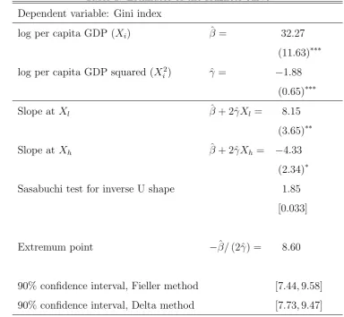
Table 1: Estimates of the Kuznets curve Dependent variable: Gini index
log per capita GDP (Xi) βˆ = 32.27
(11.63)∗∗∗
log per capita GDP squared (X2
i) ˆγ = −1.88
(0.65)∗∗∗
Slope at Xl βˆ+ 2ˆγXl= 8.15
(3.65)∗∗
Slope at Xh βˆ+ 2ˆγXh = −4.33
(2.34)∗
Sasabuchi test for inverse U shape 1.85
[0.033]
Extremum point −β/ˆ (2ˆγ) = 8.60
90% confidence interval, Fieller method [7.44,9.58]
90% confidence interval, Delta method [7.73,9.47]
Robust standard errors in parenthesis and p-values in square brackets.
***, ** and * denotes significant at the 1%, 5%, and 10% level.
relevant when looking for a U shape. As we have argued above, the individual significance
of ˆγ is always a necessary condition in the test of a U shape.
4
Illustration
As a concrete illustration of our methodology, we use a recent study by Chambers (2007).
The paper contains a standard Kuznets regression between GDP and inequality. The
data are an unbalanced panel of 29 countries giving a total of 232 observations. We
have information on the level of inequality measured by the Gini coefficient, log of PPP
adjusted GDP per capita, and a set of control variables (see Chambers (2007) for details).
Results from the regression analysis, test statistics from the Sasabuschi-test, and the
test the significance of ˆβ and ˆγ, which in this case yields a t-values of 2.77 and 2.89. With
the appropriate Sasabuchi-test, however, we see that the test for a positive slope at xh
yields a t-value of only 1.85 and hence a p-value of 0.032 with the required one-sided test.
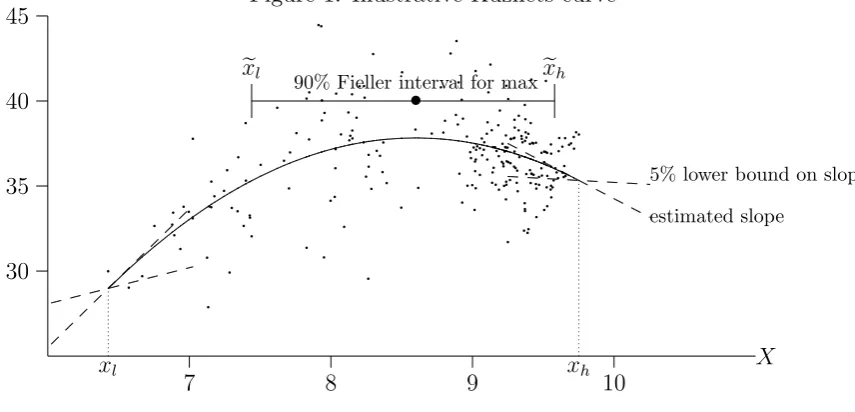
Figure 1 illustrates the estimated relationship4
, the confidence interval for the
maxi-mum and the two lower bounds on the slopes in each endpoint. We see that the turning
point of the relationship is quite close to xh, and that the slope of the curve at xh is
negative, but not very steep and only just significant at the 5% level. Hence there is a
significant hump shaped relationship over the range of the data, but the significance of
[image:10.595.81.509.298.504.2]this relationship is weaker than what would be detected by traditional approaches.
Figure 1: Illustrative Kuznets curve
7 8 9 10
30 35 40 45 X · ·· · ··· · ··· · · · ·· · · · · · ·· · · · · ·· · · · · · · · · · · · ·· · · · · ·· · · · · · · ·· · ··· · · · · · · · · · · ·· · · · · · · · · · ·· · · · · · · · · · · · ·· · · · · · · · ···· · · ····· · · · · · · · · · · · · · · · · · ·· · ··· · · ·· · · · · · · · · ··· · · · ·· · · · · ·· ···· · · · ·· · · · · · · · · · · · · · ·· ·· ·· · · · ··· · · · · ·· · · · · · · · · · ··· · ·· ··· · · ··· ... . ... ... . ... . ... ... ... . ... ... ... . ... . ... . ... ... ... . ... . ... ... ... . . ... .
...5% lower bound on slope
estimated slope
•
90% Fieller interval for maxexh
e
xl
xh
xl
5
Conclusion
In this paper we have provided an appropriate test of a U shaped relationship in a
re-gression model. In the applied econometrics literature a large number of articles tries to
identify non-monotone relationships using regression analysis. Hardly any of these use
adequate formal procedures when they test for the presence of a U shape. To the best
of our knowledge none has used the simple test that we are suggesting. Most works,
nevertheless, seems to be on fairly safe ground when they claim to have found a U shape.
The reason is that the common practice is to check two necessary conditions, namely that
the second derivative has the right sign and that the extremum point is within the data
4
range. This criteria will be misleading, however, if the estimated extremum point is too
close to the end point of the data range. Our test gives the exact necessary and sufficient
conditions for the test of a U shape. In addition, the interval interpretation provides a
References
Abiad, Abdul and Ashoka Mody (2006) “Financial Reform: What Shakes It? What
Shapes It?” American Economic Review, 95/1, pp 66 - 88
Aghion, Philippe, Nick Bloom, Richard Blundell, Rachel Griffith and Peter Howitt. (2005)
“Competition and Innovation: An Inverted-U Relationship.” Quarterly Journal of
Economics, 120, May: 701-28.
Aghion, Philippe, Rachel Griffith and Peter Howitt. (2006) “The Roots of Innovation:
Vertical Integration and Competition” American Economic Review Vol. 96, No. 2
(P&P), pp. 97-102.
Calmfors, L., and J. Driffill (1988): “Centralization of wage bargaining.”Economic Policy
6: 14-61.
Carr, David L, James R. Markusen, and Keith E. Maskus (2001) “Estimating the
Knowledge-Capital Model of the Multinational Enterprise”American Economic
Re-view, Vol. 91, No. 3 pp. 693-708
Casella, G., and R. L. Berger (2002): Statistical Inference. 2nd ed. Pacific Grove, CA:
Duxbury Press.
Chambers, D. (2007): “Trading places: Does past growth impact inequality?” Journal of
Development Economics. 82, 1. pp. 257-266.
Doveh, E., A. Shapiro, and P. D. Feigin (2002): “Testing og monotonicity in parametric
regression models.” Journal of Statistical Planning and Inference 107: 289-306.
Grossman, G. M., and A. B. Krueger (1995): “Economic growth and the environment.”
Quarterly Journal of Economics 110: 353-77.
Hegre, H., T. Ellingsen, S. Gates, and N. P. Gleditsch (2001) “Toward a democratic civil
peace? Democracy, political change, and civil war, 1816–1992.” American Political
Science Review 95: 17–33.
Imbs, Jean and Romain Wacziarg (2003) “Stages of Diversification” American Economic
Review, Vol. 93, No. 1. pp. 63-86.
Kalemli-Ozcan, Sebnem, Bent E. Sørensen, and Oved Yosha (2003) “Risk Sharing and
Industrial Specialization: Regional and International Evidence”American Economic
Kuznets, S. (1955): “Economic growth and income inequality:”American Economic
Re-view 45: 1-28.
McKinnish, Terra G. (2004) “Gender in Policy and the Labor Market Occupation,
Sex-Integration, and Divorce” American Economic Review, Vol. 94, No. 2 (P&P), pp.
322-325.
Nelson,Richard R. (1956) “A Theory of the Low-Level Equilibrium Trap in
Underdevel-oped Economies”American Economic Review Vol. 46, No. 5, pp. 894-908
Sasabuchi, S. (1980): ”A test of a multivariate normal mean with composite hypotheses
determined by linear inequalities.” Biometrika 67: 429-39.
Selden, T. M., and D. Song (1994): “Environmental quality and development: Is there
a Kuznets curve for air pollution emissions?” Journal of Environmental Economics
and Management 27: 147-62.
Sigman, Hilary (2002) “International Spillovers and Water Quality in Rivers: Do