Global Optimization by Differential Evolution and Particle Swarm Methods: Evaluation on Some Benchmark Functions

(1)

Munich Personal RePEc Archive

Global Optimization by Differential

Evolution and Particle Swarm Methods:

Evaluation on Some Benchmark

Functions

Mishra, SK

5 October 2006

(2)

SK Mishra Dept. of Economics North-Eastern Hill University Shillong, Meghalaya (India)

I. A Brief History of Optimization Research: The history of optimization of

real-valued non-linear functions (including linear ones), unconstrained or constrained, goes

back to Gottfried Leibniz, Isaac Newton, Leonhard Euler and Joseph Lagrange.

However, those mathematicians often assumed differentiability of the optimand as well

as constraint functions. Moreover, they often dealt with the equality constraints. Richard

Valentine (1937) and William Karush (1939), however, were perhaps the first

mathematicians to study optimization of nonlinear functions under inequality constraints.

Leonid Kantorovich and George Dantzig are well known for developing and popularizing

linear programming, which ushered a new era of ‘operations research’, a branch of

mathematical science that specializes in optimization. The development of linear

programming soon prompted the study of the optimization problem of nonlinear

functions (often under linear or nonlinear constraints). The joint work of Harold Kuhn

and Albert Tucker (1951) – that was backed up by the work of Karush – is a landmark in

the history of optimization of nonlinear functions.

Initially, optimization of nonlinear functions was methodologically based on the

Leibniz-Newton principles and therefore could not easily escape local optima. Hence, its

development to deal with nonconvex (multimodal) functions stagnated until the mid

1950’s. Stanislaw Ulam, John von Neumann and Nicolas Metropolis had in the late

1940’s proposed the Monte Carlo method of simulation and it was gradually realized that

the simulation approach could provide an alternative methodology to mathematical

investigations in optimization. George Box (1957) was perhaps the first mathematician

who exploited the idea and developed his evolutionary method of nonlinear optimization.

Almost a decade later, MJ Box (1965) developed his complex method, which strews

random numbers over the entire domain of the decision variables and therefore has a

great potentiality to escape local optima and locate the global optimum of a nonlinear

function. The simplex method of John Nelder and Roger Mead (1964) also incorporated

the ability to learn from its earlier search experience and adapt itself to the topography of

the surface of the optimand function.

(3)

fitness’ repeatedly. The genetic algorithms may claim to have ushered the new era of

global optimization.

A little later, in 1978, Aimo Törn introduced his “Clustering Algorithm” of global

optimization. The method improves upon the earlier local search algorithms that needed

‘multiple start’ from several points distributed over the whole optimization region.

Multi-start is certainly one of the earliest global procedures used. It has even been used in local

optimization for increasing the confidence in the obtained solution. However, one

drawback of Multi-start is that when many starting points are used, the same minimum

will eventually be determined several times. In order to improve the efficiency of

Multi-start this should be avoided. The clustering method of Törn avoids this repeated

determination of local minima. This is realized in three steps, which may be iteratively

used. The three steps are: (i) sample points in the region of interest,

(ii) transform the sample to obtain points grouped around the local minima, and (iii)

use a clustering technique to recognize these groups (i.e. neigbourhoods of the local

minima). If the procedure employing these steps is successful, then, starting a single

local optimization from each cluster would determine the local minima and, thus, also the

global minimum. The advantage in using this approach is that the work spared by

computing each minimum just once can be spent on computations in (i) and (ii), which

will increase the probability that the global minimum will be found.

(4)

annealing schedule. A wrong choice of the initial ‘temperature’, or the rate of fall in the

‘temperature’ leads to quenching or entrapment of the solution in the local minima. The

method does not provide any clear guideline as to the choice of the ‘annealing schedule’

and often requires judgment or trial and error. If the schedule is properly chosen, the

process attains the global minimum. It is said that using this method is an art and requires

a lot of experience and judgment.

A little later, Fred Glover (1986) introduced his ‘Tabu Search’ method. This

method economizes on repeated visits to the already visited points and in some sense is

close to the clustering algorithms. Glover attributes it's origin to about 1977. The basic

concept of Tabu Search as described by Glover is "a meta-heuristic superimposed on

another heuristic. The overall approach is to avoid entrainment in cycles by forbidding or

penalizing moves which take the solution, in the next iteration, to points in the solution

space previously visited ( hence "tabu"). The Tabu method was partly motivated by the

observation that human behavior appears to operate with a random element that leads to

inconsistent behavior given similar circumstances. As Glover points out, the resulting

tendency to deviate from a charted course, might be regretted as a source of error but can

also prove to be source of gain. The Tabu method operates in this way with the exception

that new courses are not chosen randomly. Instead the Tabu search proceeds according to

the supposition that there is no point in accepting a new (poor) solution unless it is to

avoid a path already investigated. This insures new regions of a problems solution space

will be investigated in with the goal of avoiding local minima and ultimately finding the

desired solution.

The pace of research in global optimization (GO) by stochastic process

accelerated considerably in the 1990’s. Marco Dorigo in his Ph.D. thesis (1992)

introduced his “Ant Colony” method of global optimization. It studies artificial systems

that take inspiration from the behaviour of real ant colonies. Ants use pheromones that

guide other fellow ants to identify the path that leads to a success. The chemical

properties of pheromones and the ability of ants to gather information and use them are

simulated in the Ant Colony method to reach at the global optimum. This method is well

suited to combinatorial (discrete) optimization problems.

(5)

and velocity are done at each iteration such that the solution often converges to the global

optimum of the function. Interestingly, this method has a very sound and

well-documented philosophical literature behind it (the British empiricist philosophy, the

American pragmatism and others like those of Friedrich Hayek, Herbert Simon, etc.).

The method of Differential Evolution (DE) grew out of Kenneth Price's attempts

to solve the Chebychev Polynomial fitting Problem that had been posed to him by Rainer

Storn. A breakthrough happened (1996), when Price came up with the idea of using

vector differences for perturbing the vector population. The crucial idea behind DE is a

scheme for generating trial parameter vectors. Initially, a population of points (p in

d-dimensional space) is generated and evaluated (i.e. f(p) is obtained) for their fitness. Then

for each point (pi) three different points (pa, pb and pc) are randomly chosen from the

population. A new point (pz) is constructed from those three points by adding the

weighted difference between two points (w(p

b

-p

c

)) to the third point (p

a

). Then this new

point (pz) is subjected to a crossover with the current point (pi) with a probability of

crossover (cr), yielding a candidate point, say pu. This point, pu, is evaluated and if found

better than p

i

then it replaces p

i

else p

i

remains. Thus we obtain a new vector in which all

points are either better than or as good as the current points. This new vector is used for

the next iteration. This process makes the differential evaluation scheme completely

self-organizing.

III. The Characteristic Features of Population-Based GO Methods: All

population-based methods of global optimization partake of the probabilistic nature inherent to them.

As a result, one cannot obtain certainty in their results, unless they are permitted to go in

for indefinitely large search attempts. Larger is the number of attempts, greater is the

probability that they would find out the global optimum, but even then it would not reach

at the certainty. Secondly, all of them adapt themselves to the surface on which they find

the global optimum. The scheme of adaptation is largely based on some guesswork since

nobody knows as to the true nature of the problem (environment or surface) and the most

suitable scheme of adaptation to fit the given environment. Surfaces may be varied and

different for different functions. A particular type of surface may be suited to a particular

method while a search in another type of surface may be a difficult proposition for it.

Further, each of these methods operates with a number of parameters that may be

changed at choice to make it more effective. This choice is often problem oriented and

for obvious reasons. A particular choice may be extremely effective in a few cases, but it

might be ineffective (or counterproductive) in certain other cases. Additionally, there is a

relation of trade-off among those parameters. These features make all these methods a

subject of trial and error exercises.

(6)

V. Some Details of the Particle Swarm Methods Used Here: In this exercise we have

used (modified) Repulsive Particle Swarm method. The Repulsive Particle Swarm

method of optimization is a variant of the classical Particle Swarm method (see

Wikipedia,

http://en.wikipedia.org/wiki/RPSO

). It is particularly effective in finding out

the global optimum in very complex search spaces (although it may be slower on certain

types of optimization problems).

In the traditional RPS the future velocity,

v

_i₊₁

of a particle at position with a recent

velocity,

v

_i

, and the position of the particle are calculated by:

1 1 2 3

1 1

ˆ

(

)

(

)

i i i i hi i

i i i

v

r x

x

r x

x

r z

x

v

ω

α

ωβ

ωγ

+

+ +

=

+

−

+

−

+

=

+

where,

• x

is the position and

v

is the velocity of the individual particle. The subscripts

i

and

i

+

1 stand for the recent and the next (future) iterations, respectively.

• r

₁

,

r r

₂ ₃

are random numbers,

∈[

0,1]

• ω

is inertia weight,

∈[

0.01,0.7]

• x

ˆ

is the best position of a particle

• x

_h

is best position of a randomly chosen other particle from within the swarm

• z

is a random velocity vector

• α β γ

,

are constants

Occasionally, when the process is caught in a local optimum, some

chaotic

perturbation in position as well as velocity of some particle(s) may be needed.

The traditional RPS gives little scope of local search to the particles. They are

guided by their past experience and the communication received from the others in the

swarm. We have modified the traditional RPS method by endowing stronger (wider)

local search ability to each particle. Each particle flies in its local surrounding and

searches for a better solution. The domain of its search is controlled by a new parameter

(nstep). This local search has no preference to gradients in any direction and resembles

closely to tunneling. This added exploration capability of the particles brings the RPS

method closer to what we observe in real life. However, in some cases moderately wide

search (nstep=9, say; see program) works better.

(7)

closer (at lesser distance) to it. But, since our particle explores the locality by itself, it is

likely that it would not benefit much from the inmates closer to it. Other relevant

topologies are : (the celebrated) ring topology,

,

star topology

,

, etc.

Now, let us visualize the possibilities of choosing (a predetermined number of)

inmates randomly from among the members of the swarm. This is much closer to reality

in the human world. When we are exposed to the mass media, we experience this.

Alternatively, we may visualize our particles visiting a public place (e.g. railway

platform, church, etc) where it (he) meets people coming from different places. Here,

geographical distance of an individual from the others is not important. Important is how

the experiences of others are communicated to us. There are large many sources of such

information, each one being selective in what it broadcasts and each of us selective in

what we attend to and, therefore, receive. This selectiveness at both ends transcends the

geographical boundaries and each one of us is practically exposed to randomized

information. Of course, two individuals may have a few common sources of information.

We have used these arguments in the scheme of dissemination of others’ experiences to

each individual particle. Presently, we have assumed that each particle chooses a

pre-assigned number of inmates (randomly) from among the members of the swarm.

However, this number may be randomized to lie between two pre-assigned limits.

VI. Some Details of the Differential Evolution Methods Used Here: The differential

Evolution method consists of three basic steps: (i) generation of (large enough)

population with N individuals [x = (x1, x2, …, xm )] in the m-dimensional space,

randomly distributed over the entire domain of the function in question and evaluation of

the individuals of the so generated by finding f(x); (ii) replacement of this current

population by a better fit new population, and (iii) repetition of this replacement until

satisfactory results are obtained or certain criteria of termination are met.

The crux of the problem lays in replacement of the current population by a new

population that is better fit. Here the meaning of ‘better’ is in the Pareto improvement

sense. A set Sa is better than another set Sb

iff :

(i)

no xi

∈

Sa is inferior to the

corresponding member of x

i∈

S

b

;

and

(ii) at least one member x

k ∈

S

a

is better than the

corresponding member xk

∈

Sb. Thus, every new population is an improvement over the

earlier one. To accomplish this, the DE method generates a candidate individual to

replace each current individual in the population. The candidate individual is obtained by

a crossover of the current individual and three other randomly selected individuals from

the current population. The crossover itself is probabilistic in nature. Further, if the

candidate individual is better fit than the current individual, it takes the place of the

current individual, else the current individual stays and passes into the next iteration. The

crossover scheme (called exponential crossover, as suggested by Kenneth Price in his

personal letter to the author) is given below. This is coded for ncross =

>

1 in the program.

The mutant vector is vi,g = xr1,g + F*(xr2,g - xr3,g) and the target vector is xi,g and the trial

vector is ui,g. The indices r1, r2 and r3 are randomly but different from each other. Uj(0,1) is a

(8)

uj,i,g = vj,i,g.

Step 3: Increment j; if j = D then reset j = 0.

Step 4: If j = jrand end crossover; else goto Step 5.

Step 5: If Cr <= Uj(0,1), then goto Step 2; else goto Step 6

Step 6: The trial vector inherits the jth parameter from the target vector, i.e., uj,i,g = xj,i,g.

Step 7: Increment j; if j = D then reset j = 0.

Step 8: If j = jrand end crossover; else goto Step 6.

There could be other schemes (as many as 10 in number) of crossover, including

no crossover (only probabilistic replacement,

NCROSS

<

=0 that works better in case of a

few functions.

VII. Specification of Adjustable Parameters: As it has been mentioned before, these

methods need certain parameters to be defined before they work. In case of the DE, we

have fixed: max number of iterations allowed, Iter = 10000, population size,

N

= 10 times

of the dimension of the function or 100 whichever maximum; scheme of crossover,

ncross =1 (defined in the program); crossover probability, pcros = 0.9; scale factor, fact =

0.5, random number seed, iu = 1111 and all random numbers are uniformly distributed

between -1000 and 1000; accuracy needed, eps =1.0e-08. If x in f(x) violates the

boundary then it is forcibly brought within the specified limits through replacing it by a

random number lying in the given limits of the function concerned. In case of the RPS:

population size,

N

=100; neighbour population,

NN

=50; steps for local search,

NSTEP

=11;

Max no. of iterations permitted,

ITRN

=10000; chaotic perturbation allowed,

NSIGMA

=1;

selection of neighbour : random,

ITOP

=3;

A1

=

A2

=0.5;

A3

=5.e-04;

W

=.5;

SIGMA

=1.e-03;

EPSI

=1.d-04. Meanings of these parameters are explained in the programs (appended).

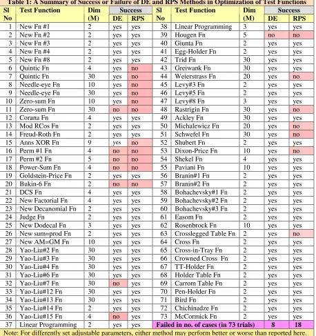
VIII. Results and Discussion: Among 70 functions, a few have been run for small as

well as large dimensions. In total, 73 optimization exercises have been done. DE has

succeeded in 65 cases while RPS has succeeded in 55 cases. In almost all cases, DE has

converged faster and given much more accurate results. The convergence of RPS is much

slower even for lesser stringency on accuracy. The summary of results is presented in

table-1. Some test functions have been hard for both the methods. These are: Zero-Sum

(30D), Perm#1, Perm#2, Power and Bukin-6 functions.

(9)

suggest that. Our purpose is not to join with the one or the other. We simply want to

highlight that in certain cases they both succeed, in certain other case they both fail and

each one has some selective preference over some particular type of surfaces. What is

needed is to identify such structures and surfaces that suit a particular method most.

[image:9.612.85.543.200.687.2]

It is needed that we find out some criteria to classify the problems that suit (or

does not suit) a particular method. This classification will highlight the comparative

advantages of using a particular method for dealing with a particular class of problems.

Table 1: A Summary of Success or Failure of DE and RPS Methods in Optimization of Test Functions

Success Success

Sl No

Test Function Dim

(M) DE RPS Sl No

Test Function Dim

(M) DE RPS

1 New Fn #1 2 yes yes 38 Linear Programming 3 yes yes

2 New Fn #2 2 yes yes 39 Hougen Fn 5 no no

3 New Fn #3 2 yes yes 40 Giunta Fn 2 yes yes

4 New Fn #4 2 yes yes 41 Egg-Holder Fn 2 yes yes

5 New Fn #8 2 yes yes 42 Trid Fn 30 yes yes

6 Quintic Fn 4 yes no 43 Greiwank Fn 30 yes yes

7 Quintic Fn 30 yes no 44 Weierstrass Fn 20 yes no

8 Needle-eye Fn 10 yes no 45 Levy#3 Fn 2 yes yes

9 Needle-eye Fn 30 yes no 46 Levy#5 Fn 2 yes yes

10 Zero-sum Fn 10 yes no 47 Levy#8 Fn 3 yes yes

11 Zero-sum Fn 30 no no 48 Rastrigin Fn 30 yes no

12 Corana Fn 4 yes yes 49 Ackley Fn 30 yes yes

13 Mod RCos Fn 2 yes yes 50 Michalewicz Fn 20 yes no

14 Freud-Roth Fn 2 yes yes 51 Schwefel Fn 30 yes no

15 Anns XOR Fn 9 yes no 52 Shubert Fn 2 yes yes

16 Perm #1 Fn 4 no no 53 Dixon-Price Fn 10 yes no

17 Perm #2 Fn 5 no no 54 Shekel Fn 4 yes yes

18 Power-Sum Fn 4 no no 55 Paviani Fn 10 yes yes

19 Goldstein-Price Fn 2 yes yes 56 Branin#1 Fn 2 yes yes

20 Bukin-6 Fn 2 no no 57 Branin#2 Fn 2 yes yes

21 DCS Fn 4 yes yes 58 Bohachevsky#1 Fn 2 yes yes

22 New Factorial Fn 4 yes yes 59 Bohachevsky#2 Fn 2 yes yes

23 New Decanomial Fn 2 yes yes 60 Bohachevsky#3 Fn 2 yes yes

24 Judge Fn 2 yes yes 61 Easom Fn 2 yes yes

25 New Dodecal Fn 3 yes yes 62 Rosenbrock Fn 10 yes yes

26 New sum=prod Fn 2 yes yes 63 Crosslegged Table Fn 2 yes no

27 New AM=GM Fn 10 yes yes 64 Cross Fn 2 yes yes

28 Yao-Liu#2 Fn 30 yes yes 65 Cross-in-Tray Fn 2 yes yes

29 Yao-Liu#3 Fn 30 yes yes 66 Crowned Cross Fn 2 yes yes

30 Yao-Liu#4 Fn 30 yes yes 67 TT-Holder Fn 2 yes yes

31 Yao-Liu#6 Fn 30 yes yes 68 Holder Table Fn 2 yes yes

32 Yao-Liu#7 Fn 30 no yes 69 Carrom Table Fn 2 yes yes

33 Yao-Liu#12 Fn 30 yes yes 70 Pen-Holder Fn 2 yes yes

34 Yao-Liu#13 Fn 30 yes yes 71 Bird Fn 2 yes yes

35 Yao-Liu#14 Fn 2 yes yes 72 Chichinadze Fn 2 yes yes

36 Yao-Liu#15 Fn 4 no yes 73 McCormick Fn 2 yes yes

37 Linear Programming 2 yes yes Failed in no. of cases (in 73 trials) 8 18

(10)

• Bauer, J.M.: “Harnessing the Swarm: Communication Policy in an Era of Ubiquitous Networks and Disruptive Technologies”, Communications and Strategies, 45, 2002.

•

Box, M.J.: “A new method of constrained optimization and a comparison with other methods”. Comp. J. 8, pp. 42-52, 1965.

• Bukin, A. D.: New Minimization Strategy For Non-Smooth Functions, Budker Institute of Nuclear Physics preprint BUDKER-INP-1997-79, Novosibirsk 1997.

• Cerny, V.: "Thermodynamical Approach to the Traveling Salesman Problem: An Efficient Simulation Algorithm", J. Opt. Theory Appl., 45, 1, 41-51, 1985.

• Eberhart R.C. and Kennedy J.: “A New Optimizer using Particle Swarm Theory”, Proceedings Sixth Symposium on Micro Machine and Human Science, pp. 39–43. IEEE Service Center, Piscataway, NJ, 1995.

• Fleischer, M.: “Foundations of Swarm Intelligence: From Principles to Practice”, Swarming Network Enabled C4ISR, arXiv:nlin.AO/0502003 v1 2 Feb 2005.

• G.E.P. Box, “Evolutionary operation: A method for increasing industrial productivity”, Applied Statistics, 6 , pp. 81-101, 1957.

• Glover F.," Future paths for Integer Programming and Links to Artificial Intelligence", Computers and Operations Research, 5:533-549, 1986.

• Hayek, F.A.: The Road to Serfdom, Univ. of Chicago Press, Chicago, 1944.

• Holland, J.: Adaptation in Natural and Artificial Systems, Univ. of Michigan Press, Ann Arbor, 1975.

• Karush, W. Minima of Functions of Several Variables with Inequalities as Side Constraints. M.Sc. Dissertation. Dept. of Mathematics, Univ. of Chicago, Chicago, Illinois, 1939.

• Kirkpatrick, S., Gelatt, C.D. Jr., and Vecchi, M.P.: "Optimization by Simulated Annealing",

Science, 220, 4598, 671-680, 1983.

• Kuhn, H.W. and Tucker, A.W.: “Nonlinear Programming”, in Neymann, J. (ed) Proceedings of Second Berkeley Symposium on Mathematical Statistics and Probability, Univ. of California Press, Berkrley, Calif. pp. 481-492, 1951.

• Metropolis, N. The Beginning of the Monte Carlo Method. Los Alamos Science, No. 15, Special Issue, pp. 125-130, 1987.

• Metropolis, N., Rosenbluth, A., Rosenbluth, M., Teller, A., and Teller, E.: "Equation of State Calculations by Fast Computing Machines", J. Chem. Phys.,21, 6, 1087-1092, 1953.

• Mishra, S.K.: “Some Experiments on Fitting of Gielis Curves by Simulated Annealing and Particle Swarm Methods of Global Optimization”, Social Science Research Network (SSRN):

http://ssrn.com/abstract=913667, Working Papers Series, 2006 (a).

• Mishra, S.K.: “Least Squares Fitting of Chacón-Gielis Curves by the Particle Swarm Method of

Optimization”, Social Science Research Network (SSRN), Working Papers Series,

http://ssrn.com/abstract=917762 , 2006 (b).

• Mishra, S.K.: “Performance of Repulsive Particle Swarm Method in Global Optimization of Some Important Test Functions: A Fortran Program” , Social Science Research Network (SSRN), Working Papers Series, http://ssrn.com/abstract=924339 , 2006 (c).

• Mishra, S.K.: “Some New Test Functions for Global Optimization and Performance of Repulsive Particle Swarm Method”, Social Science Research Network (SSRN) Working Papers Series,

http://ssrn.com/abstract=927134, 2006 (d).

• Mishra, S.K.: “Repulsive Particle Swarm Method on Some Difficult Test Problems of Global Optimization” ,SSRN: http://ssrn.com/abstract=928538 , 2006 (e).

• Nagendra, S.: Catalogue of Test Problems for Optimization Algorithm Verification, Technical Report 97-CRD-110, General Electric Company, 1997.

• Nelder, J.A. and Mead, R.: “A Simplex method for function minimization” Computer Journal, 7: pp. 308-313, 1964.

(11)

• Prigogine, I. and Strengers, I.: Order Out of Chaos: Man’s New Dialogue with Nature, Bantam Books, Inc. NY, 1984.

• Silagadge, Z.K.: “Finding Two-Dimensional Peaks”, Working Paper, Budkar Insttute of Nuclear Physics, Novosibirsk, Russia, arXive:physics/0402085 V3 11 Mar 2004.

• Simon, H.A.: Models of Bounded Rationality, Cambridge Univ. Press, Cambridge, MA, 1982. • Smith, A.: The Theory of the Moral Sentiments, The Adam Smith Institute (2001 e-version), 1759. • Sumper, D.J.T.: “The Principles of Collective Animal Behaviour”, Phil. Trans. R. Soc. B. 361, pp.

5-22, 2006.

• Törn, A.A and Viitanen, S.: “Topographical Global Optimization using Presampled Points”, J. of Global Optimization, 5, pp. 267-276, 1994.

• Törn, A.A.: “A search Clustering Approach to Global Optimization” , in Dixon, LCW and Szegö, G.P. (Eds) Towards Global Optimization – 2, North Holland, Amsterdam, 1978.

• Tsallis, C. and Stariolo, D.A.: “Generalized Simulated Annealing”, ArXive condmat/9501047 v1 12 Jan, 1995.

• Valentine, R.H.: Travel Time Curves in Oblique Structures, Ph.D. Dissertation, MIT, Mass, 1937. • Veblen, T.B.: "Why is Economics Not an Evolutionary Science" The Quarterly Journal of

Economics, 12, 1898.

• Veblen, T.B.: The Theory of the Leisure Class, The New American library, NY. (Reprint, 1953), 1899.

• Vesterstrøm, J. and Thomsen, R.: “A comparative Study of Differential Evolution, Particle Swarm Optimization, and Evolutionary Algorithms on Numerical Benchmark Problems”, Congress on Evolutionary Computation, 2004. CEC2004, 2, pp. 1980-1987, 2004.

• Whitley, D., Mathias, K., Rana, S. and Dzubera, J.: “Evaluating Evolutionary Algorithms”,

Artificial Intelligence, 85, pp. 245-276, 1996.

(12)

1: C MAIN PROGRAM : PROVIDES TO USE REPULSIVE PARTICLE SWARM METHOD

2: C (SUBROUTINE RPS) AND DIFFERENTIAL WVOLUTION METHOD (DE)

3: c ---4: c Adjust the parameters suitably in subroutines DE and RPS

5: c When the program asks for parameters, feed them suitably

6: c ---7: PROGRAM DERPS

8: IMPLICIT DOUBLE PRECISION (A-H, O-Z)

9: COMMON /KFF/KF,NFCALL ! FUNCTION CODE AND NO. OF FUNCTION CALLS 10: CHARACTER *30 METHOD(2)

11: CHARACTER *1 PROCEED

12: DIMENSION XX(2,50),KKF(2),MM(2),FMINN(2)

13: DIMENSION X(50)! X IS THE DECISION VARIABLE X IN F(X) TO MINIMIZE

14: C M IS THE DIMENSION OF THE PROBLEM, KF IS TEST FUNCTION CODE AND

15: C FMIN IS THE MIN VALUE OF F(X) OBTAINED FROM DE OR RPS

16: WRITE(*,*)'Adjust the parameters suitably in subroutines DE & RPS' 17: WRITE(*,*)'==================== WARNING =============== ' 18: METHOD(1)=' : DIFFERENTIAL EVALUATION'

19: METHOD(2)=' : REPULSIVE PARTICLE SWARM' 20: DO I=1,2

21:

22: IF(I.EQ.1) THEN

23: WRITE(*,*)'============ DIFFERENTIAL EVOLUTION PROGRAM ==========' 24: WRITE(*,*)'TO PROCEED TYPE ANY CHARACTER AND STRIKE ENTER'

25: READ(*,*) PROCEED

26: CALL DE(M,X,FMINDE) ! CALLS DE AND RETURNS OPTIMAL X AND FMIN 27: FMIN=FMINDE

28: ELSE

29: WRITE(*,*)' ' 30: WRITE(*,*)' '

31: WRITE(*,*)'==========REPULSIVE PARTICLE SWARM PROGRAM ==========' 32: WRITE(*,*)'TO PROCEED TYPE ANY CHARACTER AND STRIKE ENTER'

33: READ(*,*) PROCEED

34: CALL RPS(M,X,FMINRPS) ! CALLS RPS AND RETURNS OPTIMAL X AND FMIN 35: FMIN=FMINRPS

36: ENDIF 37: DO J=1,M 38: XX(I,J)=X(J) 39: ENDDO

40: KKF(I)=KF 41: MM(I)=M 42: FMINN(I)=FMIN 43: ENDDO

44: WRITE(*,*)' ' 45: WRITE(*,*)' '

46: WRITE(*,*)'--- FINAL RESULTS==================' 47: DO I=1,2

48: WRITE(*,*)'FUNCT CODE=',KKF(I),' FMIN=',FMINN(I),' : DIM=',MM(I) 49: WRITE(*,*)'OPTIMAL DECISION VARIABLES : ',METHOD(I)

50: WRITE(*,*)(XX(I,J),J=1,M)

51: WRITE(*,*)'/////////////////////////////////////////////////////' 52: ENDDO

53: WRITE(*,*)'PROGRAM ENDED' 54: END

55: C

---56: SUBROUTINE DE(M,A,FBEST)

57: C PROGRAM: "DIFFERENTIAL EVOLUTION ALGORITHM" OF GLOBAL OPTIMIZATION

58: C THIS METHOD WAS PROPOSED BY R. STORN AND K. PRICE IN 1995. REF

--59: C "DIFFERENTIAL EVOLUTION - A SIMPLE AND EFFICIENT ADAPTIVE SCHEME 60: C FOR GLOBAL OPTIMIZATION OVER CONTINUOUS SPACES" : TECHNICAL REPORT

61: C INTERNATIONAL COMPUTER SCIENCE INSTITUTE, BERKLEY, 1995.

62: C PROGRAM BY SK MISHRA, DEPT. OF ECONOMICS, NEHU, SHILLONG (INDIA)

63: C

---64: C PROGRAM EVOLDIF

(13)

2/36 DERPS.f

10/8/2006 6:28:30 AM

68: PARAMETER(IPRINT=500,EPS=1.d-08)!FOR WATCHING INTERMEDIATE RESULTS

69: C IT PRINTS THE INTERMEDIATE RESULTS AFTER EACH IPRINT ITERATION AND

70: C EPS DETERMINES ACCURACY FOR TERMINATION. IF EPS= 0, ALL ITERATIONS

71: C WOULD BE UNDERGONE EVEN IF NO IMPROVEMENT IN RESULTS IS THERE.

72: C ULTIMATELY "DID NOT CONVERGE" IS REOPORTED.

73: COMMON /RNDM/IU,IV ! RANDOM NUMBER GENERATION (IU = 4-DIGIT SEED) 74: INTEGER IU,IV ! FOR RANDOM NUMBER GENERATION

75: COMMON /KFF/KF,NFCALL ! FUNCTION CODE AND NO. OF FUNCTION CALLS 76: CHARACTER *70 FTIT ! TITLE OF THE FUNCTION

77: C

---78: C THE PROGRAM REQUIRES INPUTS FROM THE USER ON THE FOLLOWING

---79: C (1) FUNCTION CODE (KF), (2) NO. OF VARIABLES IN THE FUNCTION (M);

80: C (3) N=POPULATION SIZE (SUGGESTED 10 TIMES OF NO. OF VARIABLES, M,

81: C FOR SMALLER PROBLEMS N=100 WORKS VERY WELL);

82: C (4) PCROS = PROB. OF CROSS-OVER (SUGGESTED : ABOUT 0.85 TO .99);

83: C (5) FACT = SCALE (SUGGESTED 0.5 TO .95 OR SO);

84: C (6) ITER = MAXIMUM NUMBER OF ITERATIONS PERMITTED (5000 OR MORE)

85: C (7) RANDOM NUMBER SEED (4 DIGITS INTEGER)

86: C

---87: DIMENSION X(NMAX,MMAX),Y(NMAX,MMAX),A(MMAX),FV(NMAX) 88: DIMENSION IR(3)

89: C

---90: C SELECT THE FUNCTION TO MINIMIZE AND ITS DIMENSION

---91: CALL FSELECT(KF,M,FTIT)

92: C SPECIFY OTHER PARAMETERS

---93: WRITE(*,*)'POPULATION SIZE [N] AND NO. OF ITERATIONS [ITER] ?' 94: WRITE(*,*)'SUGGESTED : N => 100 OR =>10.M; ITER 10000 OR SO' 95: READ(*,*) N,ITER

96: WRITE(*,*)'CROSSOVER PROBABILITY [PCROS] AND SCALE [FACT] ?' 97: WRITE(*,*)'SUGGESTED : PCROS ABOUT 0.9; FACT=.5 OR LARGER BUT < 1' 98: READ(*,*) PCROS,FACT

99: WRITE(*,*)'RANDOM NUMBER SEED ?'

100: WRITE(*,*)'A FOUR-DIGIT POSITIVE ODD INTEGER, SAY, 1171' 101: READ(*,*) IU

102:

103: NFCALL=0 ! INITIALIZE COUNTER FOR FUNCTION CALLS 104: GBEST=1.D30 ! TO BE USED FOR TERMINATION CRITERION 105: C INITIALIZATION : GENERATE X(N,M) RANDOMLY

106: DO I=1,N 107: DO J=1,M

108: CALL RANDOM(RAND)

109: X(I,J)=(RAND-.5D00)*2000

110: C RANDOM NUMBERS BETWEEN -RRANGE AND +RRANGE (BOTH EXCLUSIVE) 111: ENDDO

112: ENDDO

113: WRITE(*,*)'COMPUTING --- PLEASE WAIT ' 114: IPCOUNT=0

115: DO 100 ITR=1,ITER ! ITERATION BEGINS 116:

117: C EVALUATE ALL X FOR THE GIVEN FUNCTION 118: DO I=1,N

119: DO J=1,M 120: A(J)=X(I,J) 121: ENDDO

122: CALL FUNC(A,M,F)

123: C STORE FUNCTION VALUES IN FV VECTOR 124: FV(I)=F

125: ENDDO

126: C ---127: C FIND THE FITTEST (BEST) INDIVIDUAL AT THIS ITERATION

128: FBEST=FV(1) 129: KB=1

130: DO IB=2,N

131: IF(FV(IB).LT.FBEST) THEN 132: FBEST=FV(IB)

(14)

135: ENDDO

136: C BEST FITNESS VALUE = FBEST : INDIVIDUAL X(KB)

137: C ---138: C GENERATE OFFSPRINGS

139: DO I=1,N ! I LOOP BEGINS

140: C INITIALIZE CHILDREN IDENTICAL TO PARENTS; THEY WILL CHANGE LATER 141: DO J=1,M

142: Y(I,J)=X(I,J) 143: ENDDO

144: C SELECT RANDOMLY THREE OTHER INDIVIDUALS 145: 20 DO IRI=1,3 ! IRI LOOP BEGINS 146: IR(IRI)=0

147:

148: CALL RANDOM(RAND) 149: IRJ=INT(RAND*N)+1

150: C CHECK THAT THESE THREE INDIVIDUALS ARE DISTICT AND OTHER THAN I 151: IF(IRI.EQ.1.AND.IRJ.NE.I) THEN

152: IR(IRI)=IRJ 153: ENDIF

154: IF(IRI.EQ.2.AND.IRJ.NE.I.AND.IRJ.NE.IR(1)) THEN 155: IR(IRI)=IRJ

156: ENDIF

157: IF(IRI.EQ.3.AND.IRJ.NE.I.AND.IRJ.NE.IR(1).AND.IRJ.NE.IR(2)) THEN 158: IR(IRI)=IRJ

159: ENDIF

160: ENDDO ! IRI LOOP ENDS

161: C CHECK IF ALL THE THREE IR ARE POSITIVE (INTEGERS) 162: DO IX=1,3

163: IF(IR(IX).LE.0) THEN

164: GOTO 20 ! IF NOT THEN REGENERATE 165: ENDIF

166: ENDDO

167: C THREE RANDOMLY CHOSEN INDIVIDUALS DIFFERENT FROM I AND DIFFERENT 168: C FROM EACH OTHER ARE IR(1),IR(2) AND IR(3)

169: C ---170: C NO CROSS OVER, ONLY REPLACEMENT THAT IS PROBABILISTIC

171: IF(NCROSS.LE.0) THEN

172: DO J=1,M ! J LOOP BEGINS 173: CALL RANDOM(RAND)

174: IF(RAND.LE.PCROS) THEN ! REPLACE IF RAND < PCROS

175: A(J)=X(IR(1),J)+(X(IR(2),J)-X(IR(3),J))*FACT ! CANDIDATE CHILD 176: ENDIF

177: ENDDO ! J LOOP ENDS 178: ENDIF

179:

180: C ---181: C CROSSOVER SCHEME (EXPONENTIAL) SUGGESTED BY KENNETH PRICE IN HIS 182: C PERSONAL LETTER TO THE AUTHOR (DATED SEPTEMBER 29, 2006)

183: IF(NCROSS.GE.1) THEN 184: CALL RANDOM(RAND) 185: 1 JR=INT(RAND*M)+1 186: J=JR

187: 2 A(J)=X(IR(1),J)+FACT*(X(IR(2),J)-X(IR(3),J)) 188: 3 J=J+1

189: IF(J.GT.M) J=1 190: 4 IF(J.EQ.JR) GOTO 10 191: 5 CALL RANDOM(RAND)

192: IF(PCROS.LE.RAND) GOTO 2 193: 6 A(J)=X(I,J)

194: 7 J=J+1

195: IF(J.GT.M) J=1 196: 8 IF (J.EQ.JR) GOTO 10 197: 9 GOTO 6

198: 10 CONTINUE 199: ENDIF

(15)

4/36 DERPS.f

10/8/2006 6:28:30 AM

202: IF(F.LT.FV(I)) THEN ! IF BETTER, REPLACE PARENTS BY THE CHILD 203: FV(I)=F

204: DO J=1,M 205: Y(I,J)=A(J) 206: ENDDO 207: ENDIF

208: ENDDO ! I LOOP ENDS 209: DO I=1,N

210: DO J=1,M

211: X(I,J)=Y(I,J) ! NEW GENERATION IS A MIX OF BETTER PARENTS AND 212: C BETTER CHILDREN

213: ENDDO 214: ENDDO

215: IPCOUNT=IPCOUNT+1

216: IF(IPCOUNT.EQ.IPRINT) THEN 217: DO J=1,M

218: A(J)=X(KB,J) 219: ENDDO

220: WRITE(*,*)(X(KB,J),J=1,M),' FBEST UPTO NOW = ',FBEST 221: WRITE(*,*)'TOTAL NUMBER OF FUNCTION CALLS =',NFCALL 222: IF(DABS(FBEST-GBEST).LT.EPS) THEN

223: WRITE(*,*) FTIT

224: WRITE(*,*)'COMPUTATION OVER' 225: RETURN

226: ELSE

227: GBEST=FBEST 228: ENDIF 229: IPCOUNT=0 230: ENDIF

231: C ---232: 100 ENDDO ! ITERATION ENDS : GO FOR NEXT ITERATION, IF APPLICABLE 233: C ---234: WRITE(*,*)'DID NOT CONVERGE. REDUCE EPS OR RAISE ITER OR DO BOTH' 235: WRITE(*,*)'INCREASE N, PCROS, OR SCALE FACTOR (FACT)'

236: RETURN 237: END

238: C ---239: C RANDOM NUMBER GENERATOR (UNIFORM BETWEEN 0 AND 1 - BOTH EXCLUSIVE) 240: SUBROUTINE RANDOM(RAND1)

241: DOUBLE PRECISION RAND1 242: COMMON /RNDM/IU,IV 243: INTEGER IU,IV 244: RAND=REAL(RAND1) 245: IV=IU*65539 246: IF(IV.LT.0) THEN 247: IV=IV+2147483647+1 248: ENDIF

249: RAND=IV 250: IU=IV

251: RAND=RAND*0.4656613E-09 252: RAND1= (RAND)

253: RETURN 254: END

255: C ---256: SUBROUTINE FSELECT(KF,M,FTIT)

257: C THE PROGRAM REQUIRES INPUTS FROM THE USER ON THE FOLLOWING ---258: C (1) FUNCTION CODE (KF), (2) NO. OF VARIABLES IN THE FUNCTION (M); 259: CHARACTER *70 TIT(100),FTIT

260: WRITE(*,*)'---' 261: DATA TIT(1)/'KF=1 NEW FUNCTION(N#1) 2-VARIABLES M=2'/

262: DATA TIT(2)/'KF=2 NEW FUNCTION(N#2) 2-VARIABLES M=2'/ 263: DATA TIT(3)/'KF=3 NEW FUNCTION(N#3) 2-VARIABLES M=2'/ 264: DATA TIT(4)/'KF=4 NEW FUNCTION(N#4) 2-VARIABLES M=2'/ 265: DATA TIT(5)/'KF=5 NEW QUINTIC FUNCTION M-VARIABLES M=?'/

(16)

269: DATA TIT(9)/'KF=9 MODIFIED RCOS FUNCTION 2-VARIABLES M=2'/ 270: DATA TIT(10)/'KF=10 FREUDENSTEIN ROTH FUNCTION 2-VARIABLES M=2'/ 271: DATA TIT(11)/'KF=11 ANNS XOR FUNCTION 9-VARIABLES M=9'/

272: DATA TIT(12)/'KF=12 PERM FUNCTION #1 (SET BETA) 4-VARIABLES M=4'/ 273: DATA TIT(13)/'KF=13 PERM FUNCTION #2 (SET BETA) M-VARIABLES M=?'/ 274: DATA TIT(14)/'KF=14 POWER-SUM FUNCTION 4-VARIABLES M=4'/

275: DATA TIT(15)/'KF=15 GOLDSTEIN PRICE FUNCTION 2-VARIABLES M=2'/ 276: DATA TIT(16)/'KF=16 BUKIN 6TH FUNCTION 2-VARIABLES M=2'/ 277: DATA TIT(17)/'KF=17 NEW FUNCTION (N#8) 2-VARIABLES M=2'/

278: DATA TIT(18)/'KF=18 DEFL CORRUG SPRING FUNCTION M-VARIABLES M=?'/ 279: DATA TIT(19)/'KF=19 NEW FACTORIAL FUNCTION M-VARIABLES M=?'/ 280: DATA TIT(20)/'KF=20 NEW DECANOMIAL FUNCTION 2-VARIABLES M=2'/ 281: DATA TIT(21)/'KF=21 JUDGE FUNCTION 2-VARIABLES M=2'/

282: DATA TIT(22)/'KF=22 NEW DODECAL FUNCTION 3-VARIABLES M=3'/ 283: DATA TIT(23)/'KF=23 NEW SUM-EQ-PROD FUNCTION 2-VARIABLES M=2'/ 284: DATA TIT(24)/'KF=24 NEW AM-EQ-GM FUNCTION M-VARIABLES M=?'/ 285: DATA TIT(25)/'KF=25 YAO-LIU FUNCTION#2 M-VARIABLES M=?'/ 286: DATA TIT(26)/'KF=26 YAO-LIU FUNCTION#3 M-VARIABLES M=?'/ 287: DATA TIT(27)/'KF=27 YAO-LIU FUNCTION#4 M-VARIABLES M=?'/ 288: DATA TIT(28)/'KF=28 YAO-LIU FUNCTION#6 M-VARIABLES M=?'/ 289: DATA TIT(29)/'KF=29 YAO-LIU FUNCTION#7 M-VARIABLES M=?'/ 290: DATA TIT(30)/'KF=30 YAO-LIU FUNCTION#12 M-VARIABLES M=?'/ 291: DATA TIT(31)/'KF=31 YAO-LIU FUNCTION#13 M-VARIABLES M=?'/ 292: DATA TIT(32)/'KF=32 YAO-LIU FUNCTION#14 2-VARIABLES M=2'/ 293: DATA TIT(33)/'KF=33 YAO-LIU FUNCTION#15 4-VARIABLES M=4'/ 294: DATA TIT(34)/'KF=34 LINEAR PROGRAMMING-I : 2-VARIABLES M=2'/ 295: DATA TIT(35)/'KF=35 LINEAR PROGRAMMING-II : 3-VARIABLES M=3'/ 296: DATA TIT(36)/'KF=36 HOUGEN FUNCTION : 5-VARIABLES M=5'/ 297: DATA TIT(37)/'KF=37 GIUNTA FUNCTION : 2-VARIABLES M=2'/ 298: DATA TIT(38)/'KF=38 EGGHOLDER FUNCTION : M-VARIABLES M=?'/ 299: DATA TIT(39)/'KF=39 TRID FUNCTION : M-VARIABLES M=?'/ 300: DATA TIT(40)/'KF=40 GRIEWANK FUNCTION : M-VARIABLES M=?'/ 301: DATA TIT(41)/'KF=41 WEIERSTRASS FUNCTION : M-VARIABLES M=?'/ 302: DATA TIT(42)/'KF=42 LEVY-3 FUNCTION : 2-VARIABLES M=2'/ 303: DATA TIT(43)/'KF=43 LEVY-5 FUNCTION : 2-VARIABLES M=2'/ 304: DATA TIT(44)/'KF=44 LEVY-8 FUNCTION : 3-VARIABLES M=3'/ 305: DATA TIT(45)/'KF=45 RASTRIGIN FUNCTION : M-VARIABLES M=?'/ 306: DATA TIT(46)/'KF=46 ACKLEY FUNCTION : M-VARIABLES M=?'/ 307: DATA TIT(47)/'KF=47 MICHALEWICZ FUNCTION : M-VARIABLES M=?'/ 308: DATA TIT(48)/'KF=48 SCHWEFEL FUNCTION : M-VARIABLES M=?'/ 309: DATA TIT(49)/'KF=49 SHUBERT FUNCTION : 2-VARIABLES M=2'/ 310: DATA TIT(50)/'KF=50 DIXON-PRICE FUNCTION : M-VARIABLES M=?'/ 311: DATA TIT(51)/'KF=51 SHEKEL FUNCTION : 4-VARIABLES M=4'/ 312: DATA TIT(52)/'KF=52 PAVIANI FUNCTION : 10-VARIABLES M=10'/ 313: DATA TIT(53)/'KF=53 BRANIN FUNCTION#1 : 2-VARIABLES M=2'/ 314: DATA TIT(54)/'KF=54 BRANIN FUNCTION#2 : 2-VARIABLES M=2'/ 315: DATA TIT(55)/'KF=55 BOHACHEVSKY FUNCTION#1 : 2-VARIABLES M=2'/ 316: DATA TIT(56)/'KF=56 BOHACHEVSKY FUNCTION#2 : 2-VARIABLES M=2'/ 317: DATA TIT(57)/'KF=57 BOHACHEVSKY FUNCTION#3 : 2-VARIABLES M=2'/ 318: DATA TIT(58)/'KF=58 EASOM FUNCTION : 2-VARIABLES M=2'/

319: DATA TIT(59)/'KF=59 ROSENBROCK FUNCTION : M-VARIABLES M=?'/ 320: DATA TIT(60)/'KF=60 CROSS-LEGGED TABLE FUNCTION:2-VARIABLES M=2'/ 321: DATA TIT(61)/'KF=61 CROSS FUNCTION : 2-VARIABLES M=2'/

322: DATA TIT(62)/'KF=62 CROSS-IN-TRAY FUNCTION : 2-VARIABLES M=2'/ 323: DATA TIT(63)/'KF=63 CROWNED CROSS FUNCTION : 2-VARIABLES M=2'/ 324: DATA TIT(64)/'KF=64 TT-HOLDER FUNCTION : 2-VARIABLES M=2'/ 325: DATA TIT(65)/'KF=65 HOLDER-TABLE FUNCTION : 2-VARIABLES M=2'/ 326: DATA TIT(66)/'KF=66 CARROM-TABLE FUNCTION : 2-VARIABLES M=2'/ 327: DATA TIT(67)/'KF=67 PENHOLDER FUNCTION : 2-VARIABLES M=2'/ 328: DATA TIT(68)/'KF=68 BIRD FUNCTION : 2-VARIABLES M=2'/

329: DATA TIT(69)/'KF=69 CHICHINADZE FUNCTION : 2-VARIABLES M=2'/ 330: DATA TIT(70)/'KF=70 MCCORMICK FUNCTION : 2-VARIABLES M=2'/

331: C ---332: DO I=1,70

333: WRITE(*,*)TIT(I) 334: ENDDO

(17)

6/36 DERPS.f

10/8/2006 6:28:30 AM

336: WRITE(*,*)'FUNCTION CODE [KF] AND NO. OF VARIABLES [M] ?' 337: READ(*,*) KF,M

338: FTIT=TIT(KF) ! STORE THE NAME OF THE CHOSEN FUNCTION IN FTIT 339: RETURN

340: END

341: C ---342: SUBROUTINE FUNC(X,M,F)

343: C TEST FUNCTIONS FOR GLOBAL OPTIMIZATION PROGRAM 344: IMPLICIT DOUBLE PRECISION (A-H,O-Z)

345: COMMON /RNDM/IU,IV 346: COMMON /KFF/KF,NFCALL 347: INTEGER IU,IV

348: DIMENSION X(*) 349:

350: PI=4.D+00*DATAN(1.D+00)! DEFINING THE VALUE OF PI 351: NFCALL=NFCALL+1 ! INCREMENT TO NUMBER OF FUNCTION CALLS 352: C KF IS THE CODE OF THE TEST FUNCTION

353: C ---354: IF(KF.EQ.1) THEN

355: C FUNCTION #1 MIN AT -0.18467 APPROX AT (-8.4666, -10) APPROX 356: F=0.D00

357: DO I=1,M

358: IF(DABS(X(I)).GT.10.D00) THEN 359: CALL RANDOM(RAND)

360: X(I)=(RAND-0.5D00)*20 361: ENDIF

362: ENDDO

363: F=DABS(DCOS(DSQRT(DABS(X(1)**2+X(2)))))**0.5 +0.01*X(1)+.01*X(2) 364: RETURN

365: ENDIF

366: C ---367: IF(KF.EQ.2) THEN

368: C FUNCTION #2 MIN = -0.199409 APPROX AT (-9.94112, -10) APPROX 369: F=0.D00

370: DO I=1,M

373: X(I)=(RAND-0.5D00)*20 374: ENDIF

375: ENDDO

376: F=DABS(DSIN(DSQRT(DABS(X(1)**2+X(2)))))**0.5 +0.01*X(1)+.01*X(2) 377: RETURN

378: ENDIF

379: C ---380: IF(KF.EQ.3) THEN

381: C FUNCTION #3 MIN = -1.01983 APPROX AT (-1.98682, -10.00000) APPROX 382: F=0.D00

383: DO I=1,M

386: X(I)=(RAND-0.5D00)*20 387: ENDIF

388: ENDDO

389: F1=DSIN(( DCOS(X(1))+DCOS(X(2)) )**2)**2 390: F2=DCOS(( DSIN(X(1))+DSIN(X(2)) )**2)**2 391: F=(F1+F2+X(1))**2 ! IS MULTIMODAL

392: F=F+ 0.01*X(1)+0.1*X(2) ! MAKES UNIMODAL 393: RETURN

394: ENDIF

395: C ---396: IF(KF.EQ.4) THEN

397: C FUNCTION #4 MIN = -2.28395 APPROX AT (2.88631, 1.82326) APPROX 398: F=0.D00

399: DO I=1,M

(18)

403: ENDIF 404: ENDDO

405: F1=DSIN((DCOS(X(1))+DCOS(X(2)))**2)**2 406: F2=DCOS((DSIN(X(1))+DSIN(X(2)))**2)**2 407: F3=-DLOG((F1-F2+X(1))**2 )

408: F=F3+0.1D00*(X(1)-1.D00)**2+0.1D00*(X(2)-1.D00)**2 409: RETURN

410: ENDIF

411: C ---412: IF(KF.EQ.5) THEN

413: C QUINTIC FUNCTION:GLOBAL MINIMA,EXTREMELY DIFFICULT TO OPTIMIZE 414: C MIN VALUE = 0 AT PERMUTATION OF (2, 2,..., 2, -1, -1, ..., -1, 415: C -0.402627941) GIVES MIN F = 0.

416: F=0.D00 417: DO I=1,M

420: X(I)=(RAND-0.5D00)*20 421: ENDIF

422: ENDDO

423: CALL QUINTIC(M,F,X) 424: RETURN

425: ENDIF

426: C ---427: IF(KF.EQ.6) THEN

428: C NEEDLE-EYE FUNCTION M=>1;

429: C MIN = 1 IF ALL ABS(X) ARE SMALLER THAN THE EYE

430: C SMALLER THE VALUE OF ZZ, MORE DIFFICULT TO ENTER THE EYE 431: C LARGER THE VALUE OF M, MORE DIFFICULT TO FIND THE OPTIMUM 432: F=0.D00

433: EYE=0.000001D00 434: FP=0.D00

435: DO I=1,M

436: IF(DABS(X(I)).GT.EYE) THEN 437: FP=1.D00

438: F=F+100.D00+DABS(X(I)) 439: ELSE

440: F=F+1.D00 441: ENDIF 442: ENDDO

443: IF(FP.EQ.0.D00) F=F/M 444: RETURN

445: ENDIF

446: C ---447: IF(KF.EQ.7) THEN

448: C ZERO SUM FUNCTION : MIN = 0 AT SUM(X(I))=0 449: F=0.D00

450: DO I=1,M

453: X(I)=(RAND-0.5D00)*20 454: ENDIF

455: ENDDO 456: SUM=0.D00 457: DO I=1,M 458: SUM=SUM+X(I) 459: ENDDO

460: IF(SUM.NE.0.D00) F=1.D00+(10000*DABS(SUM))**0.5 461: RETURN

462: ENDIF

463: C ---464: IF(KF.EQ.8) THEN

465: C CORANA FUNCTION : MIN = 0 AT (0, 0, 0, 0) APPROX 466: F=0.D00

467: DO I=1,M

(19)

8/36 DERPS.f

10/8/2006 6:28:30 AM

470: X(I)=(RAND-0.5D00)*2000 471: ENDIF

472: ENDDO 473: DO J=1,M

474: IF(J.EQ.1) DJ=1.D00 475: IF(J.EQ.2) DJ=1000.D00 476: IF(J.EQ.3) DJ=10.D00 477: IF(J.EQ.4) DJ=100.D00 478: ISGNXJ=1

479: IF(X(J).LT.0.D00) ISGNXJ=-1

480: ZJ=(DABS(X(J)/0.2D00)+0.49999)*ISGNXJ*0.2D00 481: ISGNZJ=1

482: IF(ZJ.LT.0.D00) ISGNZJ=-1

483: IF(DABS(X(J)-ZJ).LT.0.05D00) THEN 484: F=F+0.15D00*(ZJ-0.05D00*ISGNZJ)**2 * DJ 485: ELSE

486: F=F+DJ*X(J)**2 487: ENDIF

488: ENDDO 489: RETURN 490: ENDIF

491: C ---492: IF(KF.EQ.9) THEN

493: C MODIFIED RCOS FUNCTION MIN=-0.179891 AT (-3.196989, 12.52626)APPRX 494: F=0.D00

495: IF(X(1).LT.-5.D00 .OR. X(1).GT.10.D00) THEN 496: CALL RANDOM(RAND)

497: X(1)=RAND*15.D00 -5.D00 498: ENDIF

499: IF(X(2).LT.0.D00 .OR. X(2).GT.15.D00) THEN 500: CALL RANDOM(RAND)

501: X(2)=RAND*15.D00 502: ENDIF

503: CA=1.D00

504: CB=5.1/(4*PI**2) 505: CC=5.D00/PI 506: CD=6.D00 507: CE=10.D00 508: CF=1.0/(8*PI)

509: F1=CA*(X(2)-CB*X(1)**2+CC*X(1)-CD)**2 510: F2=CE*(1.D00-CF)*DCOS(X(1))*DCOS(X(2)) 511: F3=DLOG(X(1)**2+X(2)**2+1.D00)

512: F=-1.0/(F1+F2+F3+CE) 513: RETURN

514: ENDIF

515: C ---516: IF(KF.EQ.10) THEN

517: C FREUDENSTEIN ROTH FUNCTION : MIN = 0 AT (5, 4) 518: F=0.D00

519: DO I=1,M

522: X(I)=(RAND-0.5D00)*20 523: ENDIF

524: ENDDO

525: F1=(-13.D00+X(1)+((5.D00-X(2))*X(2)-2)*X(2))**2 526: F2=(-29.D00+X(1)+((X(2)+1.D00)*X(2)-14.D00)*X(2))**2 527: F=F1+F2

528: RETURN 529: ENDIF

530: C ---531: IF(KF.EQ.11) THEN

532: C ANNS XOR FUNCTION (PARSOPOULOS, KE, PLAGIANAKOS, VP, MAGOULAS, GD 533: C AND VRAHATIS, MN "STRETCHING TECHNIQUE FOR OBTAINING GLOBAL 534: C MINIMIZERS THROUGH PARTICLE SWARM OPTIMIZATION")

(20)

537: F=0.D00 538: DO I=1,M

541: X(I)=(RAND-0.5D00)*2 542: ENDIF

543: ENDDO

544: F11=X(7)/(1.D00+DEXP(-X(1)-X(2)-X(5))) 545: F12=X(8)/(1.D00+DEXP(-X(3)-X(4)-X(6))) 546: F1=(1.D00+DEXP(-F11-F12-X(9)))**(-2) 547: F21=X(7)/(1.D00+DEXP(-X(5)))

548: F22=X(8)/(1.D00+DEXP(-X(6)))

549: F2=(1.D00+DEXP(-F21-F22-X(9)))**(-2) 550: F31=X(7)/(1.D00+DEXP(-X(1)-X(5))) 551: F32=X(8)/(1.D00+DEXP(-X(3)-X(6)))

552: F3=(1.D00-(1.D00+DEXP(-F31-F32-X(9)))**(-1))**2 553: F41=X(7)/(1.D00+DEXP(-X(2)-X(5)))

554: F42=X(8)/(1.D00+DEXP(-X(4)-X(6)))

555: F4=(1.D00-(1.D00+DEXP(-F41-F42-X(9)))**(-1))**2 556: F=F1+F2+F3+F4

557: RETURN 558: ENDIF

559: C ---560: IF(KF.EQ.12) THEN

561: C PERM FUNCTION #1 MIN = 0 AT (1, 2, 3, 4)

562: C BETA => 0. CHANGE IF NEEDED. SMALLER BETA RAISES DIFFICULY 563: C FOR BETA=0, EVERY PERMUTED SOLUTION IS A GLOBAL MINIMUM 564: BETA=50.D00

565: F=0.D00 566: DO I=1,M

567: IF(DABS(X(I)).GT.M) THEN 568: CALL RANDOM(RAND)

569: X(I)=(RAND-0.5D00)*2*M 570: ENDIF

571: ENDDO 572: DO K=1,M 573: SUM=0.D00 574: DO I=1,M

575: SUM=SUM+(I**K+BETA)*((X(I)/I)**K-1.D00) 576: ENDDO

577: F=F+SUM**2 578: ENDDO 579: RETURN 580: ENDIF

581: C ---582: IF(KF.EQ.13) THEN

583: C PERM FUNCTION #2 MIN = 0 AT (1/1, 1/2, 1/3, 1/4,..., 1/M) 584: C BETA => 0. CHANGE IF NEEDED. SMALLER BETA RAISES DIFFICULY 585: C FOR BETA=0, EVERY PERMUTED SOLUTION IS A GLOBAL MINIMUM 586: BETA=10.D00

587: DO I=1,M

590: X(I)=(RAND-.5D00)*2 591: ENDIF

592: SGN=X(I)/DABS(X(I)) 593: ENDDO

594: F=0.D00 595: DO K=1,M 596: SUM=0.D00 597: DO I=1,M

598: SUM=SUM+(I+BETA)*(X(I)**K-(1.D00/I)**K) 599: ENDDO

(21)

10/36 DERPS.f

10/8/2006 6:28:30 AM

604: C ---605: IF(KF.EQ.14) THEN

606: C POWER SUM FUNCTION; MIN = 0 AT PERM(1,2,2,3) FOR B=(8,18,44,114) 607: C 0 =< X <=4

608: F=0.D00 609: DO I=1,M

610: C ANY PERMUTATION OF (1,2,2,3) WILL GIVE MIN = ZERO 611: IF(X(I).LT.0.D00 .OR. X(I).GT.4.D00) THEN

612: CALL RANDOM(RAND) 613: X(I)=RAND*4 614: ENDIF 615: ENDDO 616: DO K=1,M 617: SUM=0.D00 618: DO I=1,M

619: SUM=SUM+X(I)**K 620: ENDDO

621: IF(K.EQ.1) B=8.D00 622: IF(K.EQ.2) B=18.D00 623: IF(K.EQ.3) B=44.D00 624: IF(K.EQ.4) B=114.D00 625: F=F+(SUM-B)**2 626: ENDDO

627: RETURN 628: ENDIF

629: C ---630: IF(KF.EQ.15) THEN

631: C GOLDSTEIN PRICE FUNCTION : MIN VALUE = 3 AT (0, -1) 632: F=0.D00

633: DO I=1,M

636: X(I)=(RAND-.5D00)*20 637: ENDIF

638: ENDDO

639: F11=(X(1)+X(2)+1.D00)**2

640: F12=(19.D00-14*X(1)+ 3*X(1)**2-14*X(2)+ 6*X(1)*X(2)+ 3*X(2)**2) 641: F1=1.00+F11*F12

642: F21=(2*X(1)-3*X(2))**2

643: F22=(18.D00-32*X(1)+12*X(1)**2+48*X(2)-36*X(1)*X(2)+27*X(2)**2) 644: F2=30.D00+F21*F22

645: F= (F1*F2) 646: RETURN 647: ENDIF

648: C ---649: IF(KF.EQ.16) THEN

650: C BUKIN'S 6TH FUNCTION MIN = 0 FOR (-10, 1) 651: C -15. LE. X(1) .LE. -5 AND -3 .LE. X(2) .LE. 3 652: IF(X(1).LT. -15.D00 .OR. X(1) .GT. -5.D00) THEN 653: CALL RANDOM(RAND)

654: X(1)=-(RAND*10+5.D00) 655: ENDIF

656: IF(DABS(X(2)).GT.3.D00) THEN 657: CALL RANDOM(RAND)

658: X(2)=(RAND-.5D00)*6 659: ENDIF

660: F=100.D0*DSQRT(DABS(X(2)-0.01D0*X(1)**2))+ 0.01D0*DABS(X(1)+10.D0) 661: RETURN

662: ENDIF

663: C ---664: IF(KF.EQ.17) THEN

665: C NEW N#8 FUNCTION (MULTIPLE GLOBAL MINIMA)

666: C MIN VALUE = -1 AT (AROUND .7 AROUND, 0.785 APPROX) 667: F=0.D00

668: DO I=1,M

(22)

671: X(I)=RAND/2.D00 672: ENDIF

673: ENDDO

674: F=-DEXP(-DABS(DLOG(.001D00+DABS((DSIN(X(1)+X(2))+DSIN(X(1)-X(2))+ 675: & (DCOS(X(1)+X(2))*DCOS(X(1)-X(2))+.001))**2)+

676: & .01D00*(X(2)-X(1))**2))) 677: RETURN

678: ENDIF

679: C ---680: IF(KF.EQ.18) THEN

681: C DEFLECTED CORRUGATED SPRING FUNCTION

682: C MIN VALUE = -1 AT (5, 5, ..., 5) FOR ANY K AND ALPHA=5; M VARIABLE 683: CALL DCS(M,F,X)

684: RETURN 685: ENDIF

686: C ---687: IF(KF.EQ.19) THEN

688: C FACTORIAL FUNCTION, MIN =0 AT X=(1,2,3,...,M) 689: CALL FACTOR1(M,F,X)

690: RETURN 691: ENDIF

692: C ---693: IF(KF.EQ.20) THEN

694: C DECANOMIAL FUNCTION, MIN =0 AT X=(2, -3) 695: DO I=1,M

698: X(I)= (RAND-0.5D00)*8 699: ENDIF

700: ENDDO

701: CALL DECANOM(M,F,X) 702: RETURN

703: ENDIF

704: C ---705: IF(KF.EQ.21) THEN

706: C JUDGE'S FUNCTION F(0.864, 1.23) = 16.0817; M=2 707: CALL JUDGE(M,X,F)

708: RETURN 709: ENDIF

710: C ---711: IF(KF.EQ.22) THEN

712: C DODECAL FUNCTION 713: CALL DODECAL(M,F,X) 714: RETURN

715: ENDIF

716: C ---717: IF(KF.EQ.23) THEN

718: C WHEN X(1)*X(2)=X(1)*X(2) ? M=2 719: CALL SEQP(M,F,X)

720: RETURN 721: ENDIF

722: C ---723: IF(KF.EQ.24) THEN

724: C WHEN ARITHMETIC MEAN = GEOMETRIC MEAN ? : M =>1 725: CALL AMGM(M,F,X)

726: RETURN 727: ENDIF

728: C ---729: IF(KF.EQ.25) THEN

730: C M =>2

731: CALL FUNCT2(M,F,X) 732: RETURN

733: ENDIF

734: C ---735: IF(KF.EQ.26) THEN

736: C M =>2

(23)

12/36 DERPS.f

10/8/2006 6:28:30 AM

738: RETURN 739: ENDIF

740: C ---741: IF(KF.EQ.27) THEN

742: C M =>2

745: ENDIF

746: C ---747: IF(KF.EQ.28) THEN

748: C M =>2

751: ENDIF

752: C ---753: IF(KF.EQ.29) THEN

754: C M =>2

757: ENDIF

758: C ---759: IF(KF.EQ.30) THEN

760: C M =>2

763: ENDIF

764: C ---765: IF(KF.EQ.31) THEN

766: C M =>2

769: ENDIF

770: C ---771: IF(KF.EQ.32) THEN

772: C M =2

775: ENDIF

776: C ---777: IF(KF.EQ.33) THEN

778: C M =4

781: ENDIF

782: C ---783: IF(KF.EQ.34) THEN

784: C LINEAR PROGRAMMING : MINIMIZATION PROBLEM : M =2 785: CALL LINPROG1(M,F,X)

786: RETURN 787: ENDIF

788: C ---789: IF(KF.EQ.35) THEN

790: C LINEAR PROGRAMMING : MINIMIZATION PROBLEM : M =3 791: CALL LINPROG2(M,F,X)

792: RETURN 793: ENDIF

794: C ---795: IF(KF.EQ.36) THEN

796: C HOUGEN FUNCTION 5 VARIABLES : M =3 797: CALL HOUGEN(X,M,F)

798: RETURN 799: ENDIF

800: C ---801: IF(KF.EQ.37) THEN

802: C GIUNTA FUNCTION 2 VARIABLES :M =2 803: CALL GIUNTA(M,X,F)

(24)

805: ENDIF

806: C ---807: IF(KF.EQ.38) THEN

808: C EGGHOLDER FUNCTION M VARIABLES 809: CALL EGGHOLD(M,X,F)

810: RETURN 811: ENDIF

812: C ---813: IF(KF.EQ.39) THEN

814: C TRID FUNCTION M VARIABLES 815: CALL TRID(M,X,F)

816: RETURN 817: ENDIF

818: C ---819: IF(KF.EQ.40) THEN

820: C GRIEWANK FUNCTION M VARIABLES 821: CALL GRIEWANK(M,X,F)

822: RETURN 823: ENDIF

824: C ---825: IF(KF.EQ.41) THEN

826: C WEIERSTRASS FUNCTION M VARIABLES 827: CALL WEIERSTRASS(M,X,F)

828: RETURN 829: ENDIF

830: C ---831: IF(KF.EQ.42) THEN

832: C LEVY-3 FUNCTION 2 VARIABLES 833: CALL LEVY3(M,X,F)

834: RETURN 835: ENDIF

836: C ---837: IF(KF.EQ.43) THEN

840: RETURN 841: ENDIF

842: C ---843: IF(KF.EQ.44) THEN

846: RETURN 847: ENDIF

848: C ---849: IF(KF.EQ.45) THEN

850: C RASTRIGIN FUNCTION M VARIABLES 851: CALL RASTRIGIN(M,X,F)

852: RETURN 853: ENDIF

854: C ---855: IF(KF.EQ.46) THEN

856: C ACKLEY FUNCTION M VARIABLES 857: CALL ACKLEY(M,X,F)

858: RETURN 859: ENDIF

860: C ---861: IF(KF.EQ.47) THEN

862: C MICHALEWICZ FUNCTION M VARIABLES 863: CALL MICHALEWICZ(M,X,F)

864: RETURN 865: ENDIF

866: C ---867: IF(KF.EQ.48) THEN

868: C SCHWEFEL FUNCTION M VARIABLES 869: CALL SCHWEFEL(M,X,F)

(25)

14/36 DERPS.f

10/8/2006 6:28:30 AM

872: C ---873: IF(KF.EQ.49) THEN

874: C SHUBERT FUNCTION 2 VARIABLES 875: CALL SHUBERT(M,X,F)

876: RETURN 877: ENDIF

878: C ---879: IF(KF.EQ.50) THEN

880: C DIXON AND PRICE FUNCTION M VARIABLES 881: CALL DIXPRICE(M,X,F)

882: RETURN 883: ENDIF

884: C ---885: IF(KF.EQ.51) THEN

886: C SHEKEL FUNCTION 4 VARIABLES 887: CALL SHEKEL(M,X,F)

888: RETURN 889: ENDIF

890: C ---891: IF(KF.EQ.52) THEN

892: C PAVIANI FUNCTION 10 VARIABLES 893: CALL PAVIANI(M,X,F)

894: RETURN 895: ENDIF

896: C ---897: IF(KF.EQ.53) THEN

898: C BRANIN FUNCTION#1 2 VARIABLES 899: CALL BRANIN1(M,X,F)

900: RETURN 901: ENDIF

902: C ---903: IF(KF.EQ.54) THEN

904: C BRANIN FUNCTION#2 2 VARIABLES 905: CALL BRANIN2(M,X,F)

906: RETURN 907: ENDIF

908: C ---909: IF(KF.EQ.55) THEN

910: C BOHACHEVSKY FUNCTION#1 2 VARIABLES 911: CALL BOHACHEVSKY1(M,X,F)

912: RETURN 913: ENDIF

914: C ---915: IF(KF.EQ.56) THEN

918: RETURN 919: ENDIF

920: C ---921: IF(KF.EQ.57) THEN

924: RETURN 925: ENDIF

926: C ---927: IF(KF.EQ.58) THEN

928: C EASOM FUNCTION#3 2 VARIABLES 929: CALL EASOM(M,X,F)

930: RETURN 931: ENDIF

932: C ---933: IF(KF.EQ.59) THEN

934: C ROSENBROCK FUNCTION M VARIABLES 935: CALL ROSENBROCK(M,X,F)

936: RETURN 937: ENDIF