A Survey on Robust Image Coding Techniques

A Survey on Robust Image Coding Techniques

Pavitra V.

Masters Scholar DECE, Department of ECE

GNITS, Jawaharlal Technological University,

Hyderabad, India

Renuka Devi S.M.

Associate Professor Department of ECE

GNITS, Jawaharlal Technological University,

Hyderabad, India

Ch. Ganapathy Reddy

Head of Department Department of ECE

GNITS, Jawaharlal Technological University,

Hyderabad, India

ABSTRACT

Packet losses decrease the quality of an image or video for multimedia applications. Robust image coding is crucial to combat packet losses, for transmission of images over non feedback networks. New CS based image coding schemes are robust against packet losses and carries CS samples of nearly equal importance. CS based coding also ensures low costs and complexity for image sensing. Hence CS based image coding techniques have some distinct advantages over traditional Forward Error Correction (FEC) techniques and Multiple Description Coding (MDC) based methods .Forward error Correction techniques are generally employed along with some transform based coding , but provides a limited error resilience. MDC methods are considered to be one of the widely used mechanisms for packet losses. Compressive sensing based methods are an alternate to MDC and are able to provide robust image coding against packet losses with large number of descriptions. Recent work takes CS as a framework and Multiple Description Coding is done to get robust image coding against packet losses. The aim of the paper is to give a brief introduction to all the above techniques and survey four different CS based image coding techniques.

General Terms

Compressive sensing (CS), error resilience, image transmission, Multiple Description Coding (MDC), packet loss, robust image compression, wavelets, sparseness

Keywords

survey, Compressive sensing, Bayesian, multi scale DWT, Inter and intra scale dependencies.

1.

INTRODUCTION

The rapid growth of wireless applications has led to increased demand of robust multimedia transmission with high quality. The available bandwidth is limited and wireless networks are prone to noise. So network reliability in wireless is often unfavorable and packet losses frequently occur. The situation is even worse in some networks, such as emergency communication or military confrontation, suffered from electromagnetic, damage, congestion or malicious attacks. Reliable transmission of high quality images through networks is highly challenging. To transmit images efficiently (because of limited bandwidth), it is a common way for image to be compressed before transmitted.

There are a number of lossy compression schemes employed on digital multimedia images. Two most important standards that evolved are JPEG and JPEG2000 [22]. JPEG employs Discrete Cosine Transform (DCT) to compact image energy and thus a fraction of significant coefficients can approximate

the original image. The JPEG 2000 is the most recent image compression standard, which is based on Discrete Wavelet Transform (DWT) and outperforms JPEG in general. Set Partitioning In Hierarchical Trees (SPIHT) [19] coding of images is another popular method used for image compression.

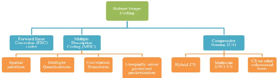
Although the existing image coding schemes can provide excellent compression performance, they also introduce high sensitivity to channel noise. One bit error or loss may cause severe error propagation and thus makes some of the bit stream that follows become meaningless [33]. Therefore, error control or data protection is necessary in many situations. In non-progressive schemes loss of a packet needs waiting for retransmission of the lost packet. There are a number of schemes defined for robust image coding in non-feedback systems (e.g., User Datagram Protocol (UDP)) that are shown in Fig 1.

The rest of the paper is organized as follows. Section I introduces the three different categories of image coding techniques and lists the papers which are surveyed. Section II introduces the concept of Compressive sensing. Section III takes up the survey of specified methods. Section IV provides comparisons and conclusion.

Section I

Images contain large volume of data. The data is spread over multiple packets even after compression. So loss of a packet causes error propagation. Forward Error Correction (FEC) [1],MDC based schemes and CS based schemes are three major types of image coding schemes which are robust against packet losses.

Forward Error Correction Codes

FEC based coding is one of the widely used channel coding techniques to control errors or lost information over noisy channels. Generally FEC methods are employed along with a Transform coding in context of Image coding. Transform based coding schemes in literature include Embedded Zero Wavelet (EZW) image coding [12], Robust quantization based image coding for transmission over noisy channels [21] .Most of these methods are wavelet based and coding is done by exploiting statistical properties of wavelet subbands. Forward error correction techniques are employed on these coded images to be robust against packet losses.

Fig 1: Robust Image coding techniques

Forward error correcting techniques become expensive as the number of errors that may occur increase.

Multiple description coding has become a good alternate for robust image coding and can withstand packet losses to some extent.

Multiple Description Coding

Multiple Description Coding (MDC) is considered as one of the effective schemes to combat packet losses over packet loss networks. In most cases, a Multiple Description (MD) coder generates two or more sub-streams referred to as descriptions, so that each description alone provides low but acceptable reconstructed quality while all the descriptions together lead to the highest quality [28]. The idea of MDC is to provide error resilience to media streams. Since an arbitrary subset of descriptions can be used to decode the original stream, network congestion or packet loss in networks such as the Internet will not interrupt the stream but only cause a (temporary) loss of quality. The quality of a stream can be expected to be roughly proportional to data rate sustained by the receiver. Combined with Multiple Path Transport (MPT), each description can be individually packetized and routed over separate physical channel. Such architecture enables traffic dispersion and can relieve Internet congestion. In the literature, a number of MDC mechanisms have been proposed, which can be roughly divided into four categories:

1) Spatial partition: The original signal is simply decomposed into more than one sub-stream in spatial or transform domain. Each subset is processed and transmitted separately. Ozarow proposed an MDC method with two channels and three receivers in the early 1980s [17]. Gamal et al. derived achievable rates for multiple descriptions [9].

2) Multiple quantizations: The output of a quantizer is assigned with two or more indexes, one for each description. Vaishampayan developed Multiple Description Scalar Quantizers (MDSQ) to overcome channel impairments [25]. Servetto et al. first proposed wavelet-based MDC using MDSQ [20]. Bai et al. presented a multiple description lattice vector quantization for wavelet image coding [2].

3) Correlation transform: The correlated information among different descriptions was harnessed. Wang et al. described an MDC technique using pair wise correlating transforms, where the correlation introduced by the transform helps to reduce the distortion when only a single description is received [27]. Lu et al. considered MDC in wavelet domain combing pair wise correlating transform with quincunx sub- sampling [16].

4) Unequally error protected packetization: Tillo et al. offered a novel R-D-based multiple description scheme compatible with JPEG2000 [23]. Yang et al. presented a However, the number of descriptions in the existing MDC schemes is very small (typically 2). Multimedia content is typically with a large amount of data and such a huge data

volume is often grouped into a number of packets. If an MDC approach has only two or three descriptions, each description would be still loaded into a lot of packets. In this scenario, packet loss in any single description can make the received packets from the description being useless and thus the decoded image quality would be severely affected. So the impact of packet loss in any single description is severe [29]. With the number of descriptions increasing, the coding complexity increases drastically and many decoders would be required. On the other hand, in the existing image coding frameworks (e.g., JPEG 2000), different portions of bit stream have different levels of significance on reconstructed quality. If the output of a source encoder could be represented with the data of equal importance in terms of information toward image reconstruction, error control would be less demanding.

Compressed Sensing

To overcome the limitations of existing MDC based algorithms the emerging Compressive Sensing (CS) theory is applied. The existing compression schemes follow „sample and then compress‟ process. When signals or images that contain high frequency components are sampled, complex systems are required to satisfy „Nyquist Criteria‟. In applications like medical scanners and radars which need high speed analog to digital converters, increasing sampling rate beyond the state-of-art is very expensive. Compressed sensing is technique to directly compress a signal or image while acquiring it. The basic idea behind compressed sensing is sparsity of natural images.

Natural images are generally sparse in basis like Discrete Cosine Transform (DCT) or Discrete Wavelet Transform (DWT). In a sparse representation, suppose a signal X of size N ×N can be represented in linear combination of just K basis vectors such that K<< N. So if a signal X is K-sparse, taking K linear measurements directly can reproduce the original signal exactly.

Even if a signal or image is not exactly K-sparse, but approximately K-sparse, taking K linear measurements can closely approximate the original signal or image. Instead of sampling the original signal at Nyquist rate and then compressing the insignificant components, compressed sensing directly takes M linear measurements while acquiring the signal when M >K such that the original signal can be closely reconstructed. This reduces significant complexity and cost of the codec.

The linear CS measurements are taken by using i.i.d (independent and identically distributed) Gaussian matrices or Rademacher matrices. By simply multiplying the signal with one of the random matrices CS measurements can be taken. The CS principle (i.e., multiplication with a random sampling matrix) can be used as an MDC framework and the CS-based MDC hassome distinctive advantages over the existing MDC schemes.

Principle (UUP), each random CS measurement is with nearly equal importance and thus can be inherently considered as one description of the original signal (i.e., CS-based coding framework is with a number of descriptions) [3].

 Secondly, the encoder of CS-based MDC is simple [29]. The generation of more than two descriptions only involves in making random measurements (i.e., multiplication with a random sampling matrix).

 Thirdly, an attractive property of CS is that the recovery quality only depends on the number of received measurements (not on which of the transmitted measurements that are received) and therefore, the proposed CS-based coding scheme has a unified decoder, while some of the existing MDC schemes employ as many as 2𝑁𝑑− 1 _{(as stated}

earlier, 𝑁𝑑is the number of descriptions) decoders.

There are several methods that have been proposed in literature that take CS measurements to code an image. As shown in fig 1 , to broadly subcategorize the methods on CS, the following categories are arrived.

 Hybrid CS : The idea was suggested by Donoho [24] , to use different algorithms for different subbands of wavelet. Han et al [10] proposed an algorithm based on hybrid CS.

 Multi Scale DWT based CS : There are a number of schemes proposed under this category where wavelet basis is primarily used for sparse representation. In regular CS, all the DWT subbands are re-measured using one CS sensing matrix. In multiscale CS, each decomposition scale is sampled separately and the number of CS measurements is allocated according to the number of wavelet coefficients.

The methods under this category can be further divided based on recovery algorithm used, the measurement matrices used and whether the measurements are adaptive or non adaptive.[30] The following algorithms are particularly considered under this category. Wang et al [29] proposed a CS based multiple description schemes where CS recovery is by solving a total variation problem. He at el [11] developed a Bayesian compressed sensing method, where a spike-and-slab prior [13] and a zero-mean Gaussian model were imposed for low-band and high-bands, respectively. Chenwei Deng et al. [6] proposed a method that uses different measurement matrices for low and high frequency subbands and uses different recovery schemes.

 CS on other bases : Other popular bases like Fourier and DCT are also used for compressed sensing. For example Fourier sinusoids based CS is used in MRI, in radar Imaging. DCT bases compressive sensing is used in computational electromagnetics.

Because of the nature of CS, all CS based methods are generally robust against packet losses. But when compared to traditional compressing methods like JPEG2000 , CS based methods results in significant penalty [8], [31].

In context of robust image coding, this paper surveys about hybrid CS and multiscale DWT based CS schemes mentioned. These multiscale DWT based CS schemes acts as CS based MDC schemes. In CS based MDC schemes, measurements are taken against equal importance of information such that each measurement will act as adescription. So the recovered image quality does not depend on the measurements that are received, instead it only depends on the number of measurements that are received. CS based MDC schemes result in good R-D performance.

Section II

2.0 Compressive Sensing Theory

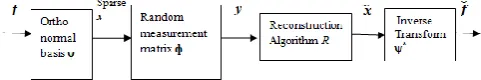
The introduction part slightly introduces the compressive sensing concept and its advantages; this section gives the mathematical details of Compressive sensing. Fig 2 shows the general block diagram for compressive sensing of a signal or image.

Consider a real valued, finite length, one dimensional discrete time signal f which can be represented as N×1 column vector in RN _{with elements f[n] where n= 1,2,3.... N. An image can} be vectorised in a higher dimension in a similar way. f can be represented in terms of a basis of N×1 vectors {𝜓i}𝑖=1𝑁 , such

that the basis is orthonormal. For an N×N basis vector

𝜓 = [𝜓1 𝜓2 … 𝜓𝑁].Then f can be expressed as shown in

equation 2.1

𝑓 = 𝑥𝑖𝜓𝑖 𝑁

𝑖=1

𝑜𝑟 𝑓 = 𝜓𝑥 (2.1)

Clearly x is the representation of f in 𝜓 domain. In the representation of x if there are only K rows that have significant coefficients then the system is said to be K sparse. If K<< N then it is clear that just K rows of x can fully represent f. This is the basic idea of transform coding. But all transform coding methods follow "sample and then compress" procedure which require a lot of resources when the signal involves high frequency information.

Fig 2: Block diagram of compressive sensing

The idea of compressive sensing is to directly take M measurements of x where M>K and M<<N such that f can be reconstructed using M linear measurements of x, represented by y. As shown in the fig 2 random measurement matrices are used for this purpose. CS theory says that from M measurements the signal can be recovered exactly if condition in 2.2 is satisfied.

𝑀 ≥ 𝐶𝑜𝑛𝑠𝑡. 𝐾. 𝑙𝑜𝑔𝑁 (2.2)

Where Const is a over measuring factor greater than 1.Once the signal is represented by linear measurements in some orthonormal basis as y, in order to get back the signal f a number of reconstruction algorithms are used. As mentioned in [26] there are different reconstructions algorithms existing in literature. There are at least five major classes of computational techniques for solving sparse approximation problems.

1) Basis pursuit : The reconstruction algorithm is defined by a convex optimization problem. Solve the convex program with algorithms that exploit the problem structure .Most popular of this is l1 minimization.

2) Greedy pursuit: Iteratively refine a sparse solution by successively identifying one or more components that yield the greatest improvement in quality.

4) Non convex optimization: Relax the „0 problem to a related non convex problem and attempt to identify a stationary point.

5) Brute force: Search through all possible support sets, possibly using cutting-plane methods to reduce the number of possibilities.

Different algorithms and their combinations are used in the methods that are to be discussed. To apply any algorithm the basic condition to be satisfied for faithful reproduction of the signal is RIP (Restricted Isometric Property). To ensure RIP the necessary condition to be satisfied is that, the measurement matrix ф is incoherent with sparsifying basis 𝜓. That is, the measurement matrix ф cannot be sparsely represented by the basis 𝜓 and vice versa.

Section III

This section surveys four robust image coding techniques.

3.1

Hybrid CS

Donoho [24] suggested a hybrid CS to measure wavelet coefficients in higher bands while using linear reconstruction for lower band. Han et al. [10] established a image representation method similar to hybrid CS which is intended for visual sensor networks.

Natural images are complex representation of real world. It is hard to find out a basis, which results in exact sparse representation of the natural image. But the natural image in general is compressible. If an image x such that f(x) = 𝜓x

,where𝜓is a orthonormal basis. x is compressed by taking K largest coefficients into account represented as 𝑥𝐾, then the

difference ||𝑥 − 𝑥𝐾||

||𝑥 − 𝑥𝐾||2 < 𝐶1 . 𝑅. 𝐾−𝑟, 𝑟 = 1/𝑝 − 1/2 ( 3.1)

where R and p are constants and depends on fn(x), that is the

n-th largest coefficients in f ( x) and coefficients of f varies as

1 ≤ 𝑛 ≤ 𝑁, 𝑓𝑛 𝑥 ≤ 𝑅. 𝑛−1/𝑝 (3.2)

Donoho [24] suggested the error bound on CS approximation reconstructed from non adaptive measurements. Given M measurements of signal x, the reconstruction error bound takes the form as shown in equation 3.3

𝑥 − 𝑥𝐶𝑆 ₂ ≤ 𝐶2 . 𝑅.

𝑀 log 𝑁

−𝑟

, 𝑟 =1 𝑝−

1 2 ( 3.3)

where C2 is a constant. If the signal is exactly sparse, the two error bounds will be at same level. Otherwise , there will be a big gap between the two error bounds. Based on these error bounds, one can observe that CS is more suited for sparse signals and if decay rate of the signal is more, it can have fast CS recovery.

Based on the analysis on error bounds, the conclusion is CS is more suited for signals with fast recovery and hence signals are sparser. So to leverage maximum signal recovery and minimum error in presence of noise the image is divided into dense and sparse components. multiscale DWT is used for this purpose. The lowest subband of DWT representation of the signals have most significant data. The coefficients decay slowly, hence it is considered as dense component.

In the other subbands the coefficients decay rate is observed to be fast. Since CS is more efficient for sparse signals, in the scheme, the input image is firstly decomposed into two components, i.e., dense and sparse components.

Fig 3 [10] shows the scheme for Hybrid CS. The input image I is first decomposed into a dense component ID and a sparse component IS through a transform T , where T could be

wavelet, curvelet, or any other transforms. In hybrid CS scheme, DWT basis W is used to decompose the image as shown in equation 3.4.

𝐼 = 𝐼𝐷+ 𝐼𝑆= 𝛼1 𝑗0,𝑘𝑊𝑗0,𝑘+ 𝛼2 𝑗 ,𝑘𝑊𝑗 ,𝑘 (3.4) 𝐾

𝑗2

𝑗 =𝑗1 𝐾

Where j0 is the coarsest level of wavelet and j1 is next level and so on. The lowest band of wavelet transform is taken as dense component and other bands as sparse components. Although the input image could be decomposed into the dense and sparse components, one can still observe that there exists a strong visual correlation between them. Therefore, it is possible to use the dense component to predict the original image, as well as the sparse component.

Fig 3: Image Representation scheme of hybrid CS

The development of adaptive interpolation provides an effective tool to solve this problem. The adaptive interpolation describe the image as a 2D piecewise autoregressive (PAR) model, as in equation 3.5

𝑋𝑖,𝑗 = 𝛽𝑚 ,𝑛 (𝑚,𝑛 )∈𝐵𝑖,𝑗

𝑋𝑖+𝑚 ,𝑗 +𝑛+ 𝑣𝑖,𝑗 (3.5)

Where (i , j) is the pixel to be interpolated, βi,j is the window

centered at pixel (i , j) , v i,j is a random perturbation

independent of pixel and the image signal.

In Zhang et al 's paper [35], they formulate the interpolation problem as an optimization problem:

min 𝑎, 𝑏, 𝑐 𝑢𝑖− 𝑎𝑡𝑣𝑖−𝑡 4 + 𝑏𝑡𝑢𝑖−𝑡 8 3

𝑡=0 2

𝑖∈𝐵

+ 𝑣_𝑖− 𝑎_𝑡𝑢_𝑖−𝑡 4 _{+ 𝑏} 𝑡𝑣𝑖−𝑡 8 3

𝑡=0 2

𝑖∈𝐵

3.6

where Iu is the image to be interpolated and the Iv is the

original image. ui & vi are pixels of image Iu and Iv

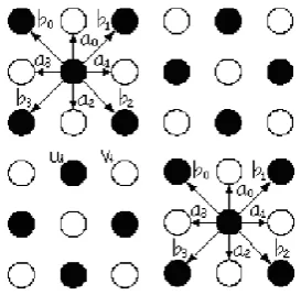
respectively. B is the window size. The superscripts (4) and (8) indicate 4-connected neighboring and 8-connected neighboring, respectively. Fig 4 [10] depicts the sample relationships.

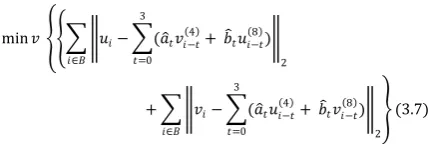
Zhang et al. [35] gives a linear least-square solution to this problem, which estimate neighboring pixels simultaneously in window B as shown in equation 3.7.

min 𝑣 𝑢𝑖− (𝑎 𝑡𝑣𝑖−𝑡 4 + 𝑏 𝑡𝑢𝑖−𝑡 8 ) 3

𝑡=0 2

𝑖∈𝐵

+ 𝑣𝑖− (𝑎 𝑡𝑢𝑖−𝑡 4 + 𝑏 𝑡𝑣𝑖−𝑡 8 ) 3

𝑡=0 2

𝑖∈𝐵

(3.7)

where 𝑎 and 𝑏 are estimated from Iu. With this interpolation

scheme ID is considered as subsample of I such that IS can be

interpolated to get back I.

The two components are measured separately. ȊD and ȊS are used to represent the dense and sparse measurements of the signal components respectively. Direct samples are taken for the dense component. In order to take measurements of the sparse components IS, a Gaussian random ensemble ϕ is used. As the dimension of the input image is very high, block based sampling strategy is used to take CS measurements of sparse component. ISis first divided into several groups by scales

and then reordered into a number of vectors of the same dimension. In the decoder side, the signal has to be recovered separately. Since the dense component is measured pixel by pixel, ȊD is exactly the wavelet coefficients of ID. Therefore, by directly applying inverse transform W‟ to ȊD will get ID. In order to recover IS, optimization problem has to be solved. The prediction Ȋ of the input image could be obtained by adaptive interpolation of the dense component by solving adaptive interpolation problem. The reconstruction of IS is based on POCS (Projection on to Convex Sets). In Candes's paper [15], they propose a different recovery procedure, which requires a small amount of priori information of the signal to be recovered but costs less computation in each iteration. In their algorithm, they assume the l1 norm of the

recovered signal is known.

In order to get a unique solution by compressed sensing the l1

ball 𝐵 = {𝑥 ∶ ||𝑥 ||𝑙1 ≤ ||𝑥||𝑙1} and the Hyper plane

𝐻 = {𝑥 ∶ 𝜙𝑥 = 𝑦} meet exactly at one point 𝐵 𝐻 = {𝑥}. because B and H are convex x can be recovered from alternate Projections On to Convex Sets (POCS) algorithm.

As the dense component ȊD is directly obtained, it is used to predict IS by adaptive interpolation. This predicted IS is used as prior signal for initialization of iteration in POCS. This predicted IS acts as a reference and helps for solution to converge more rapidly and accurately.

The main advantage of Hybrid CS scheme is separating the image into dense and sparse components and taking CS measurements for only those components that are suitable. Also prediction of the input by adaptive interpolation of dense component ensures reconstruction of image in lesser iterations. Hybrid CS method also provides high coding efficiency as the low band coefficients are JPEG 2000 encoded.

Hybrid CS method works excellently well in low PLR environments. However, with the PLR Hybrid CS cannot reconstruct original image with good quality.

3.2

CS based MDC by solving total

variation problem (TV)

Wang et al. [29] proposed a CS-MDC by solving the minimum Total Variation (TV) problem. The scheme is intended for network multimedia communication where the end devices have resource constraints and bandwidth constraints.

Existing MDC based schemes are practically restricted to 2 or 3 descriptions. So each description is still loaded into a lot of packets. So loss of packets will still pose a problem. Priority encoded transmission (PET) offers a way of generating an MDC code of fine description granularity. It can produce many packets, each of which by itself can be transmitted as a description. But the PET technique requires the source code to be rate-distortion scalable. Only few of compression standards are scalable. Moreover, the PET encoder is computationally very expensive because it needs to optimally packetize scalable source code stream. This makes PET-based MDC technique unsuitable for applications with resource constraints. In order to combat packet losses even in resource constrained network multimedia transmission, the CS based MDC scheme by solving Total Variation problem is defined.

Fig 5 : Encoder

3.2.1

Encoder

The Schematic diagram of CS-MDC encoder is as shown in Fig 5[29]. The CS-MDC encoder generates multiple descriptions simply by making random measurements of the signal f such that y = ф f, where f is a sparse representation of input image on some basis.(Wavelet basis used in the current algorithm). The matrix ф can be formed of many possible random bases, e.g., all entries of ф can be Gaussian random variables of zero mean and unit variance, or the Rademacher random variables. For the synchronization of the encoder and decoder, the random matrix ф is formed by a pseudo random number generator.

The CS measurements are real values and need to be quantized for digital communication. Because the random measurements are i.i.d. and obey a Gaussian distribution of rather high entropy, they can be coded by a uniform scalar quantizer of fixed code length without entropy coding. The absence of entropy coding will not incur heavy loss in coding efficiency while greatly simplifying the encoder and the packetization process. In the event of transmission bit errors, the fixed length code will also isolate the errors in the affected measurement without causing error avalanches. A number of coded measurements are packed into a packet and transmitted to the receiver via a lossy network.

If the random measurements are taken on the entire image, the data will be huge and computationally difficult to solve the linear programming model . So the image f is partitioned into workable sized blocks H. For example 16×16 blocks are formed with H=256. So that for each block the decoder will work reducing the time complexity of the decoder.

Measurement allocation :

To address the problem of how many measurements have to be taken for each block, the sparsity of each block is considered. Clearly even allocation of measurements is suboptimal. So relation between number of measurements m and reconstruction error function e(m) is considered. Empirically the relation is found to be 𝑒(𝑚) = 𝛽 𝑚−𝛼 where β and α are constants. β represents energy of the block and α represents decay rate. β and α are related to the coefficients

{𝜃𝑖}1≤𝑖≤𝑁 in sparse space. They can be determined by the

maximal absolute value |𝜃|𝑚𝑎𝑥 and variance ζ of the coefficients.

parameters in block b be βb and αb. The solution to the

allocation problem is given by equation 3.8

𝑚𝑏 =

𝛽1 𝛼1

𝛽𝑏𝛼𝑏𝑚1 −𝛼1−1

− _1+𝛼1 𝑏

1 ≤ 𝑏 ≤ 𝐵 (3.8)

where m1 and mb are bits allocated for 1st and bth block

respectively.

In order to compute the optimized measurement allocation, the decoder needs estimated the error functions e(m) = βm−α for all blocks. To facilitate this, | θ |max and σ are transmitted to the decoder as the side information. If we quantize these values into Q levels, the overhead of the side information is negligible, being only 2log2 Q/H bits per sample.

Quantization :

Though the length of code word is uniform , the quantization step size is varied among the block in order to minimize the quantization distortion of measurements. Quantization step size in each block depends on the variance of measurements taken in that block. The variance of measurements in each block in turn is proportional to energy f the block. So variance can be estimated for each block by the decoder. Based on the same quantization step size is estimated. No side information is needed for decoding quantization step size.

Packetization :

Although each CS measurement can be considered to be a description by itself, it cannot be transmitted on its own for the payload of data packet in network communication is much larger than the code length l of a CS measurement. A set of coded measurements are packed into a data packet and delivered to the receiver via the network. In order to solve the problem of identifying missed packet at random, the unit interval [0,1] is partitioned into B subintervals in proportion to mb. At the run time, both CS-MDC encoder and decoder use a

pseudo random number generator in [0,1] to select measurements from the B blocks, according to which subintervals the random numbers fall into. The selected measurements are packed into consecutive data packets in the pseudo random sequence.

3.2.2

Decoder

The CS-MDC decoder is even simpler. It first unpacks received packets, then performs inverse quantization and finally reconstructs the signal from the decoded measurements by solving the optimization problem. Fig 6[29] shows the block diagram of decoder.

Fig 6: Block diagram of Decoder

At decoder the problem of l1 minimization is converted into

a Total variation problem(minimum TV). The general l1

minimization problem for CS is defined as

𝑃1: 𝑚𝑖𝑛 ||𝜓𝑇𝑓||𝑙1 𝑠. 𝑡 𝜙𝑓 = 𝑦 (3.9)

When the CS measurements are corrupted with noise

𝑦 = 𝜙𝑓 + 𝑒 , ||𝑒||2 ≤ 𝜖 , where 𝜖 is the energy of the noise.

Then P1 problem will have slightly varied form.

𝑃1′: 𝑚𝑖𝑛 ||𝜓𝑇𝑓||𝑙1 𝑠. 𝑡 || 𝜙𝑓 − 𝑦||𝑙2≤ 𝜖 (3.10)

For a natural image signal fm,n, the discrete gradient is small

in most locations. In this case, the objective function in (3.10)

can be changed to minimum total variation problem of the signal || f ||TV , namely

𝑃𝑇𝑉: 𝑚𝑖𝑛 ||𝑓||𝑇𝑉 𝑠. 𝑡 || 𝜙𝑓 − 𝑦||𝑙2≤ 𝜖 (3.11)

where

||𝑓||𝑇𝑉 = 𝑚,𝑛 (𝑓𝑚 +1,𝑛− 𝑓𝑚 ,𝑛)2 + (𝑓𝑚 ,𝑛+1− 𝑓𝑚 ,𝑛)2 =

|∇𝑓𝑚 ,𝑛|

𝑚 ,𝑛 .

By solving the above optimization problem at the decoder side on each workable block , in any sparse basis, the original image can be recovered.

Compared with Other MDC based schemes, CS-MDC has a better granularity and lower complexity and can resist the packet losses efficiently. Furthermore, the decoder can reconstruct the signal in different space flexibly, which can help improve the performance for the signal which has many kinds of features in different parts.

However the R-D performance of the CS-MDC algorithm is relatively poor as the method does not fully exploit the inter and intra correlation dependencies .

3.3

Bayesian Compressive Sensing

He et al. [11] developed a Bayesian compressed sensing method, where a spike-and-slab prior [5] and a zero-mean Gaussian model were imposed for low-band and high-bands, respectively. The inter-scale dependency of high-bands has been applied for hierarchical Bayesian learning. The basis for this method is based on the statistical properties of wavelet coefficients. Wavelet coefficients results in parent children relationships. The wavelet coefficients at the coarsest scale serve as “root nodes” for the quad trees, with the finest scale of coefficients constituting the “leaf nodes”. For most natural images the negligible wavelet coefficients tend to be clustered together; specifically, if a wavelet coefficient at a particular scale is negligible, then its children are also generally (but not always) negligible. This leads to the concept of “zero trees” [19] in which a tree or sub tree of wavelet coefficients are all collectively negligible.

The structure in the wavelet coefficients is imposed within a Bayesian prior, and the analysis yields a full posterior density function on the wavelet coefficients. Consequently, in addition to estimating the underlying wavelet transform coefficients of the given image (Ѳ),“error bars” are also provided, which provide a measure of confidence in the inversion. Such error bars are useful for at least two reasons: (i) when inference is performed subsequently on Ѳ, one may be able to place that inference within the context of the confidence in the CS inversion;

(ii) typically one may not know a priori how many transform coefficients are important in a signal of interest, and therefore one will generally not know in advance the proper number of CS measurements N – one may use the error bars on the inversion to infer when enough CS measurements have been performed to achieve a desired accuracy. Let X be an M dimensional signal or image , which is sparse on wavelet basis vector ψ, an M×M basis. The CS measurement 𝑣 =ф𝜓𝑇_{𝑥 =}

ф𝜃 , where ф is a N×M (N<<M) dimensional matrix of random projections. 𝜃 denotes M dimensional vector of wavelet transform coefficients. Suppose m coefficients of θ are significant and other M-m coefficients are negligible. Then 𝜃 = 𝜃𝑚+ 𝜃𝑒 where 𝜃𝑚 represents the original 𝜃 with

M-m smallest coefficients set to zero. 𝜃𝑒 represents the m

approximated. So 𝜃𝑒 component is considered as noise ne . Further a noise component n0 is considered such that

𝑣 = ф𝜃𝑚+ 𝑛 (3.12)

where elements of n can be represented by a zero-mean Gaussian noise with unknown variance 𝜎2 , or unknown precision 𝛼𝑛= 𝜎−2.

3.3.1

TSW Modeling

Tree-structured wavelet compressive sensing (TSW-CS) model is constructed in a hierarchical Bayesian learning framework. In this setting a full posterior density function on the wavelet coefficients is inferred. Within the Bayesian framework , a spike - and - slab model is imposed for Bayesian regression. The prior for the ith element of θ (corresponding to ith transform coefficient) has the form shown in equation 3.13.

θi ~ 1 − πi δ0 + πi 𝒩 0, αi−1 , i = 1,2, . . M, (3.13)

which has 2 components. The first component δ0 is a point mass concentrated at zero, and the second component is a zero-mean Gaussian distribution with (relatively small) precision α_i−1. the former represents the zero coefficients in θ and the latter the non-zero coefficients. This is a two-component mixture model, and the two two-components are associated with the two states in the HMT [7]. The mixing weight πi, the precision parameter αi, as well as the unknown

noise precision αn, are learned from the data. The proposed Bayesian tree-structured wavelet (TSW) CS model is summarized as follows.

v θ

, αn ~ 𝒩 фθ, αn−1I , (3.14a)

θs,i ~ 1 − πs,i δ0 + πs,i 𝒩 0, αs−1 , with πs,i

=

πr , if s = 1

πs0 , if 2 ≤ s ≤ L, θpa s,i = 0

πs1 , if 2 ≤ s ≤ L, θpa s,i ≠ 0

(3.14b)

αn ~ Gamma a0, b0 , (3.14c)

αs ~ Gamma c0, d0 , s = 1,2, … … L (3.14d)

πr ~ Beta e0r, f0r , (3.14e)

πs0 ~ Beta e0s0, f0s0 , s = 2, … … L (3.14f)

πs1 ~ Beta e0s1, f0s1 , s = 2, … … L (3.14g)

where θs,i denotes the ith wavelet coefficient (corresponding

to the spatial location) at scale s, for i= 1,2...,MS (MS is the total number of wavelet coefficients at scale s) ,πs,i is the

associated mixing weight, and θpa s,i denotes the parent

coefficient of θ s,i . In (3.14b) it is assumed that all the nonzero coefficients at scale s share a common precision parameter αs. It is also assumed that all the coefficients at

scale s with a zero-valued parent share a common mixing weight πs0, and the coefficients at scale s with a nonzero

parent share a mixing weight πs1.

Gamma priors are placed on the noise precision parameter αn

and the nonzero coefficient precision parameter αs, and the posteriors of these precisions are inferred according to the data. The mixing weights πr, πs0,πs1 are also inferred, by

placing beta priors on them. To impose the structural information, depending on the scale and the parent value of the coefficients, different Beta priors are placed. For the

coefficients at the root node, a prior preferring a value close to one is set in (3.14e), because at the low-resolution level many wavelet coefficients are nonzero; for the coefficients with a zero-valued parent, a prior preferring zero is considered in (3.14f), to represent the propagation of zero coefficients across scales; finally, (3.14g) is for the coefficients with a nonzero parent, and hence no particular preference is considered since zero or nonzero values are both possible.

3.3.3

MCMC Inference

The posterior computation is implemented by an Markov chain Monte Carlo (MCMC) method [18] based on Gibbs sampling, where the posterior distribution is approximated by a sufficient number of samples. These samples are collected by iteratively drawing each random variable (model parameters and intermediate variables) from its conditional posterior distribution given the most recent values of all the other random variables. The priors of the random variables are set independently as

P αn, αs S=1:L, πr, π0s, π1s S=2:L = Gamma a0, b0

{ Gamma(c0, d0)} Beta(e0r, f0r)} Beta e0 s0_{, f}

0s0

∗ Beta(e0s1, f0s1) L

s=2

L

s=1

(3.15)

Under this setting the priors are conjugate to the likelihoods, and the conditional posteriors used to draw samples can be derived analytically. At each MCMC iteration, θ can be sampled in block manner or sequentially. But the observation is sequential sampling results in faster convergence.

3.3.4

Extensions to scaling coefficients

The TSW-CS model presented in section 3.3.2 only performs inversion for the wavelet coefficients, assuming that the scaling-function coefficients are measured separately. However, TSW model can be extended to scaling coefficients as well. The model is same as in 3.3.2 except the following,

θs,i ~ 1 − πs,i δ0 + πs,i 𝒩 0, αs−1 , with πs,i

=

πsc, if s = 0

πr , if s = 1

πs0 , if 2 ≤ s ≤ L, θpa s,i = 0

πs1 , if 2 ≤ s ≤ L, θpa s,i ≠ 0

πsc ~ Beta e0sc, f0sc , (3.16b)

Compared to the equation (3.14b) , (3.16a) is defined for s=0 as well with a mixing weight πsc, which is drawn from a prior

distribution Beta e0sc, f0sc . Considering that the scaling coefficients are usually nonzero, the hyper parameters are specified such that πsc = 1 is almost always true.

The TSW-CS method outperforms conventional wavelet based CS schemes as the intra scale correlation of DWT is also exploited. The method is able to produce very good R-D performance with low number of CS measurements.

However, the TSW-CS method cannot achieve high R-D performance, since such CS recovery schemes have not fully exploited the correlation of multi scale DWT [4].

3.4

Wavelet CS with different Low and

High Measurements

3.4.1

Encoding

The encoder and decoder of the system is as shown in fig 7 [6]. A 4 level 9/7 Daubechies DWT is used for sparse representation of the image. The low and high frequency subbands are measured differently with 2 different measurement matrices. As the lowest frequency subband of DWT contains most significant data, more measurements are taken for Low frequency subbands.

3.4.1.1

Discrete Wavelet Transform

DWT decomposes image into a set of basis functions called wavelets i.e into four bands called LL, HL, LH, HH. Here multiscale 2-D DWT is applied.

3.4.1.2

Measurements Sampling

In the proposed CS based MDC image coding instead of directly coding the DWT coefficients, they are re-sampled towards equal importance of information. In the proposed method, i.i.d. Gaussian is selected as CS measurement matrices. In this process low frequency subbands and high frequency sub bands are re-sampled separately, such that the overall re sampled information is of equal important for all subbands.

3.4.1.3

Side Information of Lower band

Coefficients

In order to identify the spatial structures existed in the low-frequency subband (denoted as LL ), we first divide LL into several 4×4 blocks at the encoder side (note that for a natural image, a 3- to 5-level wavelet decomposition is performed and the number of scaling coefficients is practically no less than16×16). For the coefficients in each block, spatial Gabor filters with different frequencies and orientations are utilized to extract the dominant orientation of structures in each block [34].

Fig 8[6] shows possible eight directions of spatial Gabor filters. By using such Gabor filters, each scaling coefficient has an output response with respective to the filter kernel and the largest response value will be selected as the representative orientation. For each block, the number of coefficients in each orientation is calculated and the orientation with the largest number of coefficients is

considered as the statistically major orientation of structures. The information of major orientation in each block corresponds to one of the eight intra predictors. This is sent to the decoder as side information using 3 bits per block. If there is no major orientation in the 4× 4 block, i.e., the outputs of the eight Gabor filters are similar, all the eight intra prediction modes are tested at the encoder side and the candidate mode with minimal Sum of Absolute Differences (SAD) or Mean Absolute Differences (MAD) of the low-band residuals is selected and the information of selected intra mode is also sent to the decoder via 3 bits per block.

3.4.1.4

Quantization and Packeting

Once CS measurements are taken for High and Low frequency sub bands, the resulting coefficients are quantized and distributed into packets and sent across the channel. The entropy coding stage is optional.

CS measurements are taken differently for high and low band coefficients separately as shown in equation

𝑌𝐿

𝑌𝐻 =

ф𝐿

ф𝐻

𝑋𝐿

𝑋𝐻 (3.17)

where 𝑌𝐻 and 𝑌𝐿 denote CS samples measured from low- and

high-bands, while 𝑋𝐿 and 𝑋𝐻represent the scaling and wavelet coefficients, respectively. Assume that L -level 2-D DWT is performed for an N -length image, the number of scaling coefficients is N/4L , which is much smaller than that of original image data . Such coefficients capture extremely important information, and therefore, almost the same number of CS samples are taken. Number of CS samples for high band wavelet coefficients is decided based on bit budget.

3.4.2

Decoding

Fig 7: Block diagram of CS based image compression

side bits are put in different packets and more copies of the overhead are transmitted to combat channel loss. For high frequency band information developed a Bayesian compressed sensing method, where a spike-and-slab prior [13] and a zero-mean Gaussian model were imposed. Using this Bayesian framework High frequency band coefficients are recovered exploiting intra dependencies among neighboring high frequency coefficients.

Fig 8 : Spatial Gabor filter kernels with eight orientations

3.4.2.1

Inverse Discrete Wavelet Transform

The Wavelet coefficients recovered in previous step are used to as inputs to recover original image f by applying Inverse Discrete Wavelet Transform.

3.4.3

Scaling Coefficients

Scaling coefficients are not sparse and nature and carry most of the significant information of an image. the strong intra-redundancy of low-frequency subband provides possibilities to make a concise representation for the scaling coefficients. For each scaling coefficient the dominant orientation is found out and for each block, the orientation with largest number of coefficients is considered as dominant orientation. This is sent as side information with 3 bits per block.

With the received CS samples and the side information of intra mode predictor, one can recover the scaling coefficients at the decoder side, by solving the following object function:

min 𝑅[𝑋𝐿(𝑠)] 𝑙1 𝑠. 𝑡 ф𝐿𝑋𝐿− 𝑌𝐿 𝑙2 ≤ 𝜖 (3.18) 1≤𝑠≤𝑆

where XL and YL denote the scaling coefficients and received CS measurements, respectively; ε represents the noise term and фL is the measurement matrix; S is the number of 4×4 blocks. R[.] depicts the residuals generated by intra-prediction using one of the eight directional modes shown in Fig 8.

3.4.4

Wavelet Coefficients Recovery

Wavelet coefficient recovery is based on Bayesian CS method explained in 3.3.2 and 3.3.3. TSW CS model is applied for sparse coefficients.

The method is referred as WLH - CS as different CS measurement matrices are used for low and high band wavelet coefficients. The method fully exploits intra and inter scale dependencies of wavelet coefficients.

Section IV

4.

COMPARISONS

Table 1 compares different CS based image coding techniques that are discussed. , CS TV represents CS based MDC by solving total variation problem. TSW-CS represents Tree structured Wavelet CS. WLH -CS represents CS based MDC using multiscale DWT with different measurements for low and high bands.

Table 1: Comparison of different methods

Method Computati onal complexit y

Application Methodology

Hybrid CS

Medium Storage based /transmission applications

with Low

PLRs.

Separately coding dense and sparse

components of

image.

CS TV Low Networks

where end

devices are resource constrained

Block based CS measurements are taken and solved by minimizing total variation problem

TSW-CS High Transmission

on networks with Low to medium PLR

Exploiting inter scale dependencies of multiscale DWT (MCMC inference for coefficients recovery)

WLH

-CS

High Transmission

on High PLR networks

Exploiting inter scale, intra scale dependencies of multiscale DWT. different recovery and measurements for low and high band coefficients

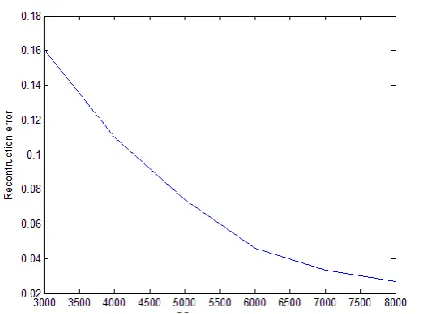
TSW -CS and WLH CS methods uses MCMC techniques and require more computational resources. However , both the methods can achieve better image quality with fewer number of CS measurements (Computationally efficient).

Fig 9:CS measurements Vs Reconstruction error for TSW-CS.

5.

CONCLUSIONS

The comparisons presented above can be summarized as follows

 Hybrid CS method is best suited for storage based applications or transmission on networks with Low packet loss rate. This method is a good compromise between coding efficiency and coding expenses, as the method exploits the properties of dense and sparse components of wavelet decomposed image.

 CS-MDC Total Variation method is best suited for visual sensor networks, where the network is resource and bandwidth constrained.

 TSW-CS method exploits the inter scale dependencies of multiscale DWT , by belief propagation. The method makes CS recovery problem to be computationally very efficient. The method is suited for image coding on networks with low to medium packet loss rates.

 WLH-CS method is best suited for image coding on networks with high to very high packet loss rates. The method fully exploits the intra and inter scale dependencies of multiscale DWT.

Previously the coding efficiency of CS based algorithms is poor compared to JPEG 2000 [8], [31]. Now by taking different measurement algorithms for low and high frequency subbands, the coding efficiency has been increased without sacrificing quality. Rate - distortion performance, Complexity of codec and Coding efficiency are considered as main parameters for devising a practical image codec which is robust against packet losses.

To resist loss of packets different algorithms are developed for duplication [6]. Also by employing different algorithms for recovery of low and high frequency sub bands, the complexity of receiver also controlled. The trend is towards algorithms with optimized R-D characteristics ,coding efficiency and error resilience with minimal computational complexity. We hope more methods that can be implementable in real time applications.

6.

REFERENCES

[1] Alexander E. Mohr, Eve A. Riskin, and Richard E. Ladner. "Unequal loss protection: Graceful degradation of image quality over packet erasure channels through forward error correction." Selected Areas in Communications, IEEE Journal on 18.6 (2000): 819-828. [2] Bai H. H., Zhu C. and Zhao Y., “Optimized multiple description lattice vector quantization for wavelet image coding,” IEEE Trans. Circuits Syst. Video Technol., vol. 17, no. 7, Jul. 2007, pp. 912–917.

[3] Candès E. J. and Tao T., “Near-optimal signal recovery from random projections: Universal encoding strategies?,” IEEE Trans. Inf. Theory,vol. 52, no. 12–54, Dec. 2006, pp. 5406–5425.

[4] Dekel S., Adaptive Compressed Image Sensing Based on Wavelet Trees, 2008. [Online]. Available: http://shaidekel.tripod.com/.

[5] Deng C.W., Lin W. S., Lee B. S. and Lau C. T., “Robust image compression based upon compressive sensing,” in Proc. IEEE Int. Conf. Multimedia and Expo. (ICME‟10), Jul. 2010, pp. 462–467.

[6] Deng C.W., Lin W. S., Lee B. S. and Lau C. T., “Robust image coding based upon compressive sensing,” Multimedia, Vol. 14, No. 2, April 2012, PP 278- 290. [7] Duarte M. F., Wakin M. B. and Baraniuk R. G.,

“Wavelet-domain compressive signal reconstruction using a hidden Markov tree model,” in Proc. IEEE Int. Conf. Acoustics, Speech. Signal Process. (ICASSP‟08), Mar. 2008, pp. 5137–5140.

[8] Fletcher A.K., Rangan S. and Goyal V. K., “On the rate-distortion performance of compressed sensing,” in Proc. IEEE Int. Conf. Acoustics, Speech. Signal Process. (ICASSP‟07), Apr. 2007, pp. 885–888.

[9] Gamal A. E. and Cover T. , “Achievable rates for multiple descriptions,” IEEE Trans. Inf. Theory, vol. 28, no. 6, Nov. 1982, pp. 851–857.

[10] Han B., Wu F., and Wu D. P., “Image representation by compressive sensing for visual sensor networks,” J. Vis. Communication., vol. 21, no. 4, May 2010, pp. 325–333. [11] He L. H and Carin L. , “Exploiting structure in wavelet-based Bayesian compressive sensing,” IEEE Trans. Signal Process., vol. 57, no. 9, Sep. 2009, pp.3488–3497. [12] Hong Man ,Kossentini, F. ; Smith, M.J.T. "Robust EZW image coding for noisy channels ",IEEE Signal Processing letters, Aug.1997, PP 227-229002E

[13] Ishwaran H. and Rao J. S., “Spike and slab variable selection: Frequentist and Bayesian strategies,” Ann. Statist., vol. 33, no. 2,Sep. 2005, pp. 730–773.

[14] Ji S. , Xue Y. , and Carin L., “Bayesian compressive sensing,” IEEE Transactions on Signal Processing, vol. 56, 2008, pp. 2346–2356.

[15] Candès E. and Romberg J., “Practical signal recovery from random projections”, Wavelet Applications in Signal and Image Processing XI, Proc. SPIE Conf., pp. 5914, 2004.

[16] Lu T. L., Shi Y. H., Kong D. H. and Yin B. C., “A wavelet-based multiple description coding combing pairwise correlating transform with quincunx sub-sampling,” in Proc. IEEE Int. Conf. Signal Process.(ICSP’08), Oct. 2008, pp. 1223–1226.

[17] Ozarow L., “On a source coding problem with two channels and three receivers,” Bell Syst. Tech. J., vol. 59, Dec. 1980, pp. 1909–1921.

[18] Robert C. P. and Casella G., Monte Carlo Statistical Methods, 2nd ed. New York: Springer, 2004.

[19] Said A. and Pearlman W. A., “A new, fast, and efficient image codec based on set partitioning in hierarchical trees,” IEEE Transactions on Circuits and Systems for Video Technology, vol. 6, 1996, pp. 243–250.

[20] Servetto S. D. ,Ramchandran K. , Vaishampayan V. A. and Nahrstedt K., “Multiple description wavelet based image coding,” IEEETrans. Image Process., vol. 9, no. 5, May 2000, pp. 813–826.

[22] Taubman D. S. and Marcellin M. W, “JPEG 2000: Standard for interactive imaging,” Proc. IEEE, vol. 90, no. 8, Aug. 2002, pp. 1336–1357.

[23] Tillo T. and Olmo G. , “A novel multiple description coding scheme compatible with the JPEG 2000 decoder,” IEEE Signal Process. Lett., vol. 11, no. 11, Nov. 2004, pp. 908–911.

[24] Tsaig Y. and Donoho D. L., “Extensions of compressed sensing,” Signal Process., vol. 86, no. 5, Jul. 2006, pp. 533–548.

[25] Vaishampayan V A., “Design of multiple description scalar quantizers,”IEEE Trans. Inf. Theory, vol. 39, no. 3, May 1993, pp. 821–834.

[26] Tropp, Joel A., and Stephen J. Wright. "Computational methods for sparse solution of linear inverse problems." Proceedings of the IEEE 98.6 (2010): 948-958.

[27] Wang Y., Orchard M. T., Vaishampayan V.A and Reibman R. , “Multiple description coding using pairwise correlating transforms,” IEEETrans. Image Process., vol. 10, no. 3, Mar. 2001, pp. 351–366. [28] Wang Y , Reibman A. R. and Lin S. N. “Multiple

description coding for video delivery,” Proc. IEEE, vol. 93, no. 1, Jan. 2005, pp. 57–70.

[29] Wang L. J., Wu X. L. and Shi G. M., “A compressive sensing approach of multiple descriptions for network multimedia communication,” in Proc. IEEE Workshop Multimedia Signal Process. (MMSP’08), Oct. 2008, vol. 1, pp. 445–449.

[30] Wu X. L. and Zhang X. J., “Model-guided adaptive recovery of compressive sensing,” in Proc. Data Compression Conf. (DCC’09), Mar.2009, pp. 123–132. [31] Wu F., Fu J. J., Lin Z. C. and Zeng B., “Analysis on

rate-distortion performance of compressive sensing for binary sparse source,” in Proc. Data Compression Conf. (DCC‟09), Mar. 2009, pp. 113–122.

[32] Yang S. H. and Cheng P. F., “Robust transmission of SPIHT-coded image over packet networks,” IEEE Trans. Circuits Syst. Video Technol., vol. 17, no. 5, May 2007, pp. 558–567.

[33] Zadeh H. Y., Jafarkhani H. And Etemadi F., “Transmission of progressive images over noisy channels: An end-to-end statistical optimization framework,” IEEE J. Select. Topics. Signal Process., vol. 2, no. 2, Nov. 1999, pp.569–571.