A New Task Scheduling Algorithm for Maximizing the Distributed Systems Efficiency

A New Task Scheduling Algorithm for Maximizing the

Distributed Systems Efficiency

Amal El-Nattat

Computer Science & Eng. Dept., Faculty of Electronic Eng.

Menouf 32952, Egypt.

Nirmeen A. El-Bahnasawy

Computer Science & Eng. Dept., Faculty of Electronic Eng.

Menouf 32952, Egypt.

Ayman El-Sayed

Computer Science & Eng. Dept., Faculty of Electronic Eng.

Menouf 32952, Egypt.

ABSTRACT

Efficient task scheduling is essential to obtain high performance in distributed computing environment. Achieving a better makespan is a key issue in designing and development of task scheduling algorithms. Several algorithms have been proposed for homogeneous and heterogeneous distributed computing systems. In this paper, we proposed a new static scheduling algorithm called Leveled DAG Prioritized Task (LDPT) to efficiently schedule tasks on homogeneous distributed computing systems. LDPT aims to improve the efficiency of the system by minimizing the schedule length.

Keywords

Task scheduling; Homogeneous distributed computing systems; Precedence constrained parallel applications; Directed Acyclic Graph.

1.

INTRODUCTION

Distributed systems have emerged as powerful platforms for executing parallel applications. They are efficient systems that are known to solve tasks and problems in a feasible and fast way. A distributed system can be defined as a computing system in which services are provided by a pool of loosely coupled computers collaborating over a network working for a common goal [1]. It can be homogeneous (in which processors are identical in capabilities and functionality) or heterogeneous (in which processors are different).

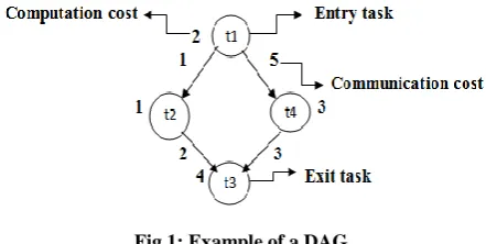
In distributed computing environment, an application is usually decomposed into several independent and/or interdependent sets of cooperating tasks. These tasks are represented by a Directed Acyclic Graph (DAG). DAG is a graph consists of a set of vertices or nodes and a set of edges G(V, E) in which each node represents a task and each edge represents a communication between two tasks (the two tasks are dependent on each other). The weight associated with each node represents the computation cost of the task and the weight associated with each edge represents the communication cost between two tasks. If two dependent tasks are executed on the same processor, then the communication cost between them is considered to equal zero. Figure 1 shows an example of a simple task graph (DAG). In the figure, t1 is called predecessor (or parent) of t2 and t2 is called successor (or child) of t1. The edge between t1 and t2 means that t2 can start execution only after t1 finishes its execution.

The efficient scheduling of application tasks is critical to achieve high performance in parallel and distributed systems. The objective function of scheduling is to map the tasks onto the processors and order their execution so that task precedence requirements are satisfied and minimum schedule length (or makespan) is obtained [2].Task-scheduling algorithms are broadly classified into two classes: static and dynamic. When the characteristics of an application, such as execution time of tasks and data dependencies between tasks are known in advance, the scheduling algorithm is known as static model.

Static task scheduling takes place during compile time before running the distributed application. Whereas in the dynamic scheduling decisions are made at run time [3].

Fig 1: Example of a DAG

Over the past few decades, research efforts are mainly focused on the problem of task scheduling on algorithms running on homogenous and heterogeneous systems mainly with the objective of reducing the overall execution time of the tasks. Topcuoglu et al. [4] have presented HEFT and CPOP scheduling algorithms for heterogonous processors. Luiz et al. [5] have developed lookahead-HEFT algorithm, which look ahead in the schedule to make scheduling decisions. Eswari, R. and Nickolas, S. [6] have proposed PHTS algorithm to efficiently schedule tasks on the heterogeneous distributed computing systems. Rajak and Ranjit [7] have presented a queue based scheduling algorithm called TSB to schedule tasks on homogeneous parallel multiprocessor system. Ahmed, S.G.; Munir, E.U.; and Nisar, W. [8] have developed genetic algorithm called PEGA that provide low time complexity than standard genetic algorithm (SGA). Xiaoyong Tang; Kenli Li; Renfa Li; and Guiping Liao [9] have presented a list-scheduling algorithm called HEFD for heterogeneous computing systems. Nasri, W. and Nafti, W. [10] have developed a new DAG scheduling algorithm for heterogeneous systems that provide better performance than some well-known existing scheduling algorithms.

The remainder of this paper is organized as follows. Section 2 provides an overview of the related work algorithm. The proposed algorithm is discussed in section 3. Section 4 presents performance evaluation results of the proposed algorithm. Section 5 introduces a discussion of energy awareness. Finally, conclusion is reviewed in section 6.

2.

RELATED WORK ALGORITHM

B-level algorithm is a list based scheduling algorithm. It depends on sorting all tasks in the graph into a list and then schedules them one by one. Before the scheduling begins, the b-level values of all tasks in a task graph are computed and sorted into a scheduling list in decreasing order of their b-level values. Then, tasks are picked from the sorted list and assigned to PMs one by one. Each task is assigned to the processor which minimize the earliest start time of that task. If LPathi=

{ni, ni+1, …,nexit} is the longest path from node ni to exit node

so the b-level value for the task ni is defined as:

b-leveli = Σ nj∈ node(LPathi) wj+Σej∈ edge(LPathi) cj ---- (1)

3.

OUR PROPOSED SCHEDULING

ALGORITHM (LDPT)

LDPT is a list based scheduling algorithm. It depends on dividing the DAG into levels with considering the dependency conditions among tasks in the DAG. The algorithm has two phases: (1) Task prioritization phase, (2) Processor selection phase.

3.1

Task Prioritization Phase:

In this phase, the DAG is divided into levels then, the tasks in each level will be sorted into a list based on their computation cost in decreasing order. The ties are broken by the communication cost between the task and all of its childs in the next level.

The priority for each task is Wj(ni) for tasks that have non

equal computation cost values or Cj[(ni)j , 𝑁𝑥=1 𝑛𝑥 j+1] for

tasks having equal computation cost values, Where Wj(ni) is

the computation cost of the specified task (ni) in the j level

where 1 ≤ j ≤ T, T is the total number of levels and 1 ≤ i ≤ N, N is the total number of tasks. Cj[(ni)j , 𝑁𝑥=1 𝑛𝑥 j+1] determines

the sum of communication costs between task (ni) in j level and

all of its children in j+1 level. A child task is denoted by (nx)

where 1≤ x ≤ N.

3.2

Processor Selection Phase:

In this phase, the tasks are picked from the list one by one and assigned to the processor that will minimize the earliest start time of the task, with taking into consideration the insertion-based policy. The insertion policy means that if there is an idle time slot on the processor between two already scheduled tasks and it was enough for executing the task, then the task is assigned on that processor in this idle slot without violating precedence constraints. In other words, a task can be scheduled earlier if there is a period of time between two tasks already scheduled on processor (P), where P runs idle. If two processors provide the same start time for the task then, the task is assigned to the processor on which most of its parents are scheduled. The Earliest Start Time of a task 𝑛𝑖on a

processor 𝑃𝑗is defined as:

EST(𝒏𝒙, 𝑷𝒎)=max[TAvailable(𝑷𝒎),max{AFT(𝒏𝒊)+𝒄𝒙,𝒊}]-- (2)

Where TAvailable (𝑃𝑚) is the earliest time at which processor

𝑃𝑚is ready. AFT(𝑛𝑖) is the Actual Finish Time of a task 𝑛𝑖 (the

parent of task nx) on the processor𝑃𝑚. 𝑐𝑛,𝑖 is the

communication cost from task 𝑛𝑖 to task 𝑛𝑥,𝑐𝑘,𝑖 equal zero if

the predecessor task 𝑡𝑘is assigned to processor 𝑃𝑚. For the

entry task, EST(𝑛𝑒𝑛𝑡𝑟𝑦, 𝑃𝑚)= 0. Figure (2) shows the pseudo

code of LDPT algorithm. Generate the DAG

Divide the DAG into levels according to their communicated dependency

Sort the constructed levels according to dependency ordering

Sort tasks according to [their computation costs then their direct communication of its next level] in descending order While there are unscheduled levels do

While there are unscheduled tasks do For each level do

Find the task with the highest computation cost If there are tasks have equal computation cost Then

Choose the task with the highest communication cost with its childs in next level

End if

Find the processor that minimizes the Earliest Start Time of the selected task

Assign the task to the selected processor Remove the selected task from the list Repeat

Until all tasks are scheduled End for each

End while

Fig 2: .Leveled DAG Prioritized Task (LDPT) algorithm.

3.3

Case Study

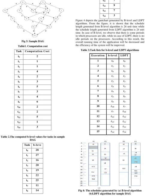
Consider the DAG shown in figure (3), assume the system has two processors (P0, P1). Table 1 shows the computation cost for each task; table 2 shows the b-level value for each task. Both b-level, LDPT algorithms generate a list of tasks that shows the execution order of them. For b-level algorithm, the tasks are sorted in the list in decreasing order according to their b-level value that is computed by using equation 1. For LDPT algorithm, the DAG is divided into levels and the tasks are sorted in each level in descending order according to their computation cost. Table 3 shows the lists generated by b-level and LDPT algorithms. Figure (4.a, 4.b) shows the gantchart generated by B-level and LDPT algorithms respectively. Both algorithms assign the selected task to the processor that minimizes the start time (EST) of it. For example, in figure 4.a, the EST for task t6 on p0 is 2 and the EST for t6 on p1 is 1, so

the task t6 is scheduled on p1. The data ready time (DRT) for task t5 on p0 is 4 and the DRT for t5 on p1 is 6, so the task is

scheduled on p0. In figure 4.b, the same manner if followed but

with taking into consideration the insertion based policy. For example, in figure 4.b, the EST for task t7 on p0 is 15 and the

EST for t7 on p1 is 18 while the DRT for t7 on p0 is 13 and the

DRT for t7 on p1 is 9. It is shown that p1 is idle from 9 to 14

and this period is enough for executing t7, so t7 is inserted in

this idle time period (between t2 and t8 ) on p1. In addition, task

that the schedule length (the finish time of the last task scheduled from the DAG) resulted from B-level and LDPT algorithms is 26, 24 unit of time respectively.

Fig 3: Sample DAG

Table1. Computation cost

Task Co mput ati on Cost

t0 2

t1 1

t2 1

t3 4

t4 2

t5 3

t6 5

t7 3

t8 4

t9 6

t10 2

t11 2

t12 5

t13 1

t14 3

Table 2.The computed b-level values for tasks in sample DAG

Task b-l eve

t0 28

t1 27

t2 16

t3 20

t4 19

t5 22

t6 25

t7 11

t8 14

t9 17

t10 14

t11 7

t12 9

t13 7

t14 3

Figure 4 depicts the gantchart generated by B-level and LDPT algorithms. From the figure, it is shown that the schedule length generated from B-level algorithm is 26 unit time while the schedule length generated from LDPT algorithm is 24 unit time. In case of B-level, we observe that there is some periods in which processors are idle, while in case of LDPT, there is no idle periods on the processors. According to this result, the overall running time of the application will be decreased and the efficiency of the system will be improved.

Table 3.Task lists for b-level and LDPT algorithms

Ex ecuti on b-l evel LDPT

1 t0 t0

2 t1 t1

3 t6 t6

4 t5 t3

5 t3 t5

6 t4 t4

7 t9 t2

8 t2 t9

9 t8 t8

10 t1 0 t7

11 t7 t1 0

12 t1 2 t1 2

13 t1 3 t1 1

14 t1 1 t1 3

15 t1 4 t1 4

4.

RESULTS AND PERFORMANCE

EVALUATION

4.1

Simulation Environment

To evaluate the performance of our developed LDPT algorithm, a simulator had been built using visual C# .NET 4.0 on machine with: Intel(R) Core(TM) i3 CPU M 350 @2.27GHz, RAM of 4.00 GB, and the operating system is window 7, 64-bit.

To test the performance of B-level and LDPT algorithms, a set of randomly generated graphs is created by varying a set of parameters that determines the characteristics of the generated DAGs. These parameters are described as follows:

DAG size (n: the number of tasks in DAG). Density (d: the probability of existence edge between ni in levelj and nx in the

next level levelj+1 for DAG. Where, i, x=1,2,…, N, and N is the

number of tasks, j=1, 2,…, T, and T is the number of levels in DAG). With six different numbers of processors varying from 2, 4, 8, 16, 32 and 64 processors. For each number of processors, six different DAG sizes have been used varying from 10, 20,40,60,80 and 100 nodes.

4.2

Evaluation Metrics

Schedule length, speed up, and efficiency are the most important metrics used for evaluating performance of scheduling algorithms. In addition, energy consumption is defined as a metric since we are focused on minimizing of the energy consumed by the PMs and NDs. Schedule length is the maximum finish time of the last task (exit task) scheduled from the DAG.

Schedule length= Max(AFT(nexit)) ---(3)

Where AFT(nexit) is the actual finish time of the exit task.Speed up is defined as the ratio of the schedule length generated from executing the application on one processor to the schedule length generated from executing the application on multiple parallel processors.

Speed up= 𝒑𝒋𝝐𝑷[ 𝒏𝒊𝝐𝑽𝒘(𝒊,𝒋)]

𝑴𝒊𝒏

𝑺𝑳 ---(4)

Where 𝑤 𝑖, 𝑗 means the weight of task ni on processor pj and SL means the schedule length. Efficiency is the inverse of speed up.

𝑬𝒇𝒇𝒊𝒄𝒊𝒆𝒏𝒄𝒚 = 𝟏

𝒔𝒑𝒆𝒆𝒅𝒖𝒑 ---(5)

4.3

Experimental Results

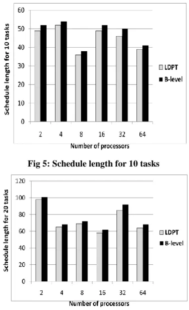
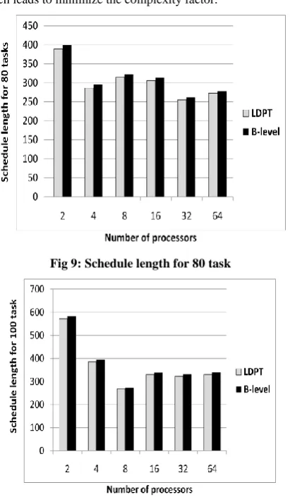
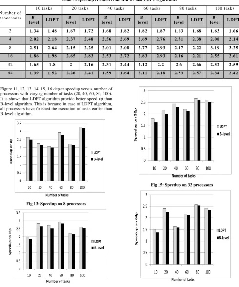
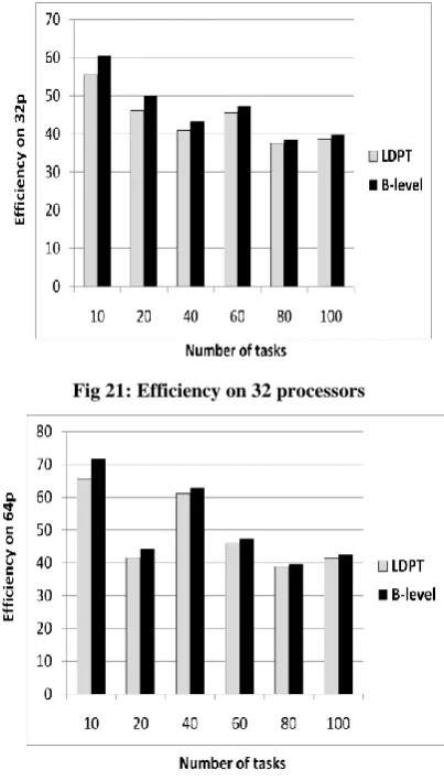
The schedule length generated by b-level and LDPT algorithms is shown in figure 5, 6, 7, 8, 9, 10 for 10, 20, 40, 60, 80, 100 tasks respectively and the results are recorded in table 4. According to the results, the schedule length is decreased that will minimize the running time of the application. The improvement ratio in schedule length is (1%). Figure 11, 12, 13, 14, 15, 16 show a comparative study of the speed up of b-level and LDPT algorithms in case of 2, 4, 8, 16, 32, 64 processors respectively. Table 5 shows the speedup results of B-level and LDPT algorithms. From the results, we can see that the improving ratio in speed up is (1.58%). From figure 17, 18, 19, 20, 21, 22 we can see that LDPT is more efficient than b-level. The improvement ratio in efficiency is (1.38%). Table 6 shows the efficiency results of B-level and LDPT algorithms.

Fig 5: Schedule length for 10 tasks

Fig 6: Schedule length for 20 tasks

Fig 7: Schedule length for 40 task

Figure 5, 6, 7, 8, 9, 10 depict the schedule length versus number of tasks with varying number of processors 2, 4, 8, 16, and 32 processors. It is shown that the schedule length in case of applying LDPT algorithm is less than B-level algorithm. This is because B-level algorithm depends on paths idea and this will increase the communication overhead during assigning tasks on processors. On the other side, LDPT algorithm depends on levels idea that will minimize the communication overhead during assigning tasks on processors. Another reason is that B-level algorithm must calculate the b-level value for each task before scheduling so that, the arithmetic calculation in LDPT is less than B-level algorithm which leads to minimize the complexity factor.

Fig 9: Schedule length for 80 task

Fig 10: Schedule length for 100 task

Fig 11: Speedup on 2 processors

Fig 12: Speedup on 4 processors

Table 4. Schedule length resulted from B-level and LDPT algorithms

Nu mber of t as ks

2 processor 4 processor 8 processor 16 processor 32 processor 64 processor

B

-level LDPT B

-level LDPT B

-level LDPT B

-level LDPT B

-level LDPT B

-level LDPT

10 52 49 54 52 38 36 52 49 50 46 41 39

20 101 98 68 65 72 69 62 58 92 85 68 64

40 210 194 127 121 163 158 131 122 149 141 218 212

60 300 293 197 192 177 167 181 175 254 245 246 239

80 399 389 295 286 322 315 313 306 261 255 278 273

Table 5. Speedup resulted from B-level and LDPT algorithms

Nu mber o f proces sors

10 tasks 20 tasks 40 tasks 60 tasks 80 tasks 100 tasks

B

-level LDPT B

-level LDPT B

-level LDPT B

-level LDPT B

-level LDPT B

-level LDPT

2 1.34 1.48 1.67 1.72 1.68 1.82 1.82 1.87 1.63 1.68 1.63 1.66 4 2.02 2.18 2.37 2.48 2.56 2.69 2.69 2.76 2.31 2.38 2.08 2.14 8 2.51 2.64 2.15 2.25 2.01 2.08 2.77 2.93 2.17 2.22 3.19 3.25 16 1.86 1.98 2.65 2.83 2.53 2.72 2.83 2.93 2.16 2.21 2.55 2.61 32 1.65 1.8 2 2.16 2.31 2.44 2.12 2.2 2.6 2.66 2.52 2.59 64 1.39 1.52 2.26 2.41 1.59 1.64 2.11 2.18 2.53 2.57 2.34 2.42

Figure 11, 12, 13, 14, 15, 16 depict speedup versus number of processors with varying number of tasks (20, 40, 60, 80, 100). It is shown that LDPT algorithm provide better speed up than B-level algorithm. This is because in case of LDPT algorithm, all processors have finished the execution of tasks earlier than B-level algorithm.

Fig 13: Speedup on 8 processors

Fig 14: Speedup on 16 processors

Fig 15: Speedup on 32 processors

Fig 17: Efficiency on 2 processors

Fig 18: Efficiency on 4 processors

Fig 19: Efficiency on 8 processors

Fig 20: Efficiency on 16 processors

Fig 21: Efficiency on 32 processors

Fig 22: Efficiency on 64 processors

Figure 17, 18, 19, 20, 21, 22 depict efficiency versus number of processors with varying number of tasks (20, 40, 60, 80, 100). It is shown that LDPT algorithm is more efficient and provide better performance than B-level algorithm. Most of processors elements have been perfect utilized in our algorithm because of the communications among tasks is not affected in algorithm breadth procedures.

5.

DISCUSSION OF ENERGY AWARENESS

EASy (Energy Aware Scheduling) algorithm is an algorithm that aims to reduce power consumption. EASy is divided into two phases. In the first phase B-level algorithm is used for scheduling. In this paper, we have developed a new static scheduling algorithm called LDPT (Leveled DAG Prioritized Task). LDPT outperforms B-level in terms of schedule length, speedup, and efficiency. The second phase of EASy algorithm involves applying a technique called DVFS (Dynamic Voltage Frequency Scaling) [18] for power reduction. We expect good results when applying LDPT instead of B-level with this technique (DVFS).

6.

CONCLUSION AND FUTURE WORK

 In this paper LDPT algorithm is applied on Directed Acyclic Graph (DAG). In the future it can be applied on Directed Cyclic Graph (DCG).

 LDPT can be applied on Heterogeneous Distributed Computing Systems (HDCS).

 LDPT can be applied in a dynamic strategy instead of static strategy.

 Finally, duplication technique can be applied with LDPT algorithm to minimize the communication overhead.

7.

REFERENCES

[1] Journal of Theoretical and Applied Information Technology. (2011, April 9). [Online]. Available: http://www.jatit.org/distributed-computing/grid-vs-distributed.htm.

[2] H. Topcuoglu, S. Hariri, and M.Y. Wu, “Performance-Effective and Low-Complexity Task Scheduling for Heterogeneous Computing,” IEEE Trans. Parallel and Distributed Systems, Vol. 13, No.3, pp. 260-274, March 2002.

[3] Y.K. Kwok and I. Ahmad, “Static Scheduling Algorithms for allocating Directed Task Graphs to Multiprocessors”, ACM Computing Surveys, Vol.31, No.4, pp. 406-471, December 1999.

[4] Topcuoglu, H., Hariri, S., Wu, M.Y. "Performance effective and low complexity task scheduling for heterogonous computing", IEEE Trans. Parallel Distributed Syst. 13(3), 2002.

[5] Luiz F. Bittencourt, Rizos Sakellariou. "DAG Scheduling Using a Look ahead Variant of the Heterogeneous Earliest Finish Time Algorithm", 18th Euromicro International Conference on Parallel, Distributed and Network-Based Processing (PDP), pp. 27-34, 2010.

[6] Eswari, R. and Nickolas, S. "Path-Based Heuristic Task Scheduling Algorithm for Heterogeneous Distributed Computing Systems". Advances in Recent Technologies in Communication and Computing (ARTCom), International Conference on 2010. P: 30-34.

[7] Rajak and Ranjit. "A Novel Approach for Task Scheduling in Multiprocessor System". International Journal of Computer Applications (IJCA), Vol.44, No. 11, pp. 12-16. April 2012.

[8] Ahmad, S.G.; Munir, E.U. and Nisar, W. PEGA "A Performance Effective Genetic Algorithm for Task

Scheduling in Heterogeneous Systems". High Performance Computing and Communication & 2012 IEEE 9th International Conference on Embedded Software and Systems (HPCC-ICESS), IEEE 14th International Conference on 2012. Pp. 1082-1087. [9] Tang, X., et al., "List scheduling with duplication for

heterogeneous computing systems", Journal of Parallel and Distributed Computing (JPDC), Vol. 70, No.4, pp. 323-329. 2010.

[10]Nasri,W. and Nafti, W. "A new DAG scheduling algorithm for heterogeneous platforms". Parallel Distributed and Grid Computing (PDGC), second IEEE International Conference on 2012. Pp. 114-119.

[11]B. Kruatrachue and T. Lewis, "Grain size determination for parallel processing," IEEE Software, vol. 5, no. 1, pp. 23-32, May 1988.

[12]M. Y. Wu and D. D. Gajski, "Hypercool: a programming aid for message passing systems," IEEE Transactions on Parallel and Distributed Systems, vol. I, no. 3 pp. 330-343, July 1990.

[13]J. J. Hwang. Y.C. Chow. F. D. Anger and C.-Y. Lee. "Scheduling precedence graphs In systems with interprocessor communication times." SLAM Journal of Computing, vol. 18, no. 2. pp. 244-257. 1989.

[14]G.C. Slh and E. A. Lee. "A compile-time scheduling heuristic for interconnection-constrained heterogeneous processor architectures." IEEE Transactions on Parallel and Distributed Systems, vol. 4. no. 2, pp. 75-87. Feb. 1997.

[15]H. El-Rewini and T.G .Lewis, " Scheduling parallel programs onto arbitrary target machines." Journal of Parallel and Distributed Computing, vol. 9. no. 2, pp. 138-153, June 1990.

[16]Panos M. Pardalos, SanguthevarRajasekaran, José D. P. Rolim, " Randomization Methods in Algorithm Design: DIMACS Workshop", vol. 43, December 12-14, 1997. [17]Ebrahimirad, V.; Rajabi, A.; Goudarzi, M., "Energy-aware

scheduling algorithm for precedence-constrained parallel tasks of network-intensive applications in a distributed homogeneous environment". Computer and Knowledge Engineering (ICCKE) 3th International Conference on 2013. Pp. 368 – 375.