Optimal Patent Breadth: Quantifying the Effects of Increasing Patent Breadth

Munich Personal RePEc Archive

Optimal Patent Breadth: Quantifying

the Effects of Increasing Patent Breadth

Chu, Angus C.

University of Michigan

July 2007

Online at

https://mpra.ub.uni-muenchen.de/3910/

Optimal Patent Breadth:

Quantifying the Effects of Increasing Patent Breadth

Angus C. Chu*

University of Michigan

July 2007

Abstract

In a generalized quality-ladder growth model, this paper firstly derives the optimal patent breadth

and the socially optimal profit-sharing arrangement between patentholders. In this general-equilibrium

setting, it identifies and derives a dynamic distortion of markup pricing on capital accumulation that has

been neglected by previous studies on patent policy. Then, it quantitatively evaluates the effects of

eliminating blocking patent and increasing patent breadth, and this exercise suggests a number of

findings. Firstly, the market economy underinvests in R&D so long as a non-negligible fraction of

long-run TFP growth is driven by R&D. Secondly, increasing patent breadth may be an effective solution to

R&D underinvestment. The resulting effect on long-run consumption can be substantial because the

harmful distortionary effects are relatively insignificant. However, the damaging effect of blocking patent

arising from suboptimal profit-sharing arrangements between patentholders can be quantitatively

significant. Finally, it considers the effect on consumption during the transition dynamics.

Keywords: endogenous growth, intellectual property rights, patent breadth, R&D JEL classification: O31, O34

*

“Although length of protection is the most obvious policy lever for governing the

profitability of an intellectual property right, it is not the instrument that shows up in

patent disputes. Patent disputes almost always revolve around either validity of the patent

in the first place, or the subtle question of how different another product must be in order

not to infringe. The latter notion is colloquially known as the ‘breadth’ of the property

right.” – Scotchmer (2004, p. 103)

1. Introduction

Patent protection in the form of patent breadth has strengthened in the United States (US) since the 80’s.1 The facts that effective patent lives are very short and only a small fraction of patents are maintained until

the end of the statutory term suggest that perhaps the term of patent is less of an important policy tool

than patent breadth.2 The first objective of this paper is to develop a tractable framework for a general-equilibrium analysis on optimal patent breadth using a quality-ladder growth model. In an environment

with sequential innovations, patent breadth takes the form of lagging breadth and leading breadth.

Lagging breadth provides patent protection against imitation while leading breadth provides patent

protection against subsequent innovations, which might infringe existing patents. Whether an increase in

leading breadth would enhance or dampen the incentives for research and development (R&D) depends

on the profit-sharing arrangement between patentholders, who may engage in a complicated bargaining

process. This paper derives the socially optimal profit-sharing arrangement between patentholders that

should be implemented by the patent authority through designing an appropriate set of institutional

policies for patent disputes to influence the patentholders’ bargaining power. Upon enforcing this optimal

profit-sharing arrangement, the optimal level of patent breadth can be determined by balancing the social

marginal cost of distortions arising from patent protection and the social marginal benefit of R&D.

1

See, e.g. Jaffe (2000), Gallini (2002), and Jaffe and Lerner (2004) for a comprehensive discussion. Hall, Jaffe and Trajtenberg (2002) provide data on the increase in the average number of patent citations, which can be viewed as a rough proxy for the broadening of patent breadth.

2

The second objective of this paper is to analyze the distortionary effects of increasing patent

breadth. The patent-design literature emphasizes the tradeoff of patent protection between the incentives

for R&D and the static distortionary effect of monopolistic markup pricing. However, mostly based on a

partial-equilibrium setting, this literature neglects an important dynamic distortion on capital

accumulation. In particular, increasing patent breath potentially raises the market value of patents on one

hand and worsens the incentives for capital accumulation on the other by increasing the wedge between

the marginal product of capital and its rental price. This paper identifies and analytically derives this

distortionary effect in a generalized version of the quality-ladder growth model originating from

Grossman and Helpman (1991) and Aghion and Howitt (1992).

The third objective of this paper is to provide a quantitative assessment on the effects of

eliminating blocking patent and increasing patent breadth. Figure 1 shows that private spending on R&D

in the US as a share of gross domestic product (GDP) has been rising sharply since the beginning of the

80’s. Then, after a few years, the number of patents granted by the US Patent and Trademark Office also

began to increase rapidly as shown in Figure 2. The calibration exercise takes as a premise the hypothesis

that the incentive for private investments in R&D increases in response to broadening patent protection

and makes use of the general-equilibrium framework to quantitatively evaluate the effects of increasing

patent breadth and R&D along with the blocking-patent, static and dynamic distortionary effects on

consumption. This numerical exercise suggests a number of findings. Firstly, the market economy

underinvests in R&D relative to the first-best optimum so long as a non-negligible fraction of long-run

total factor productivity (TFP) growth is driven by R&D. The quality-ladder growth model involves

multiple externalities in R&D investment: (a) a negative intratemporal congestion or duplication

externality; (b) a positive or negative externality in intertemporal knowledge spillover; (c) the

monopolists’ static surplus appropriability problem which is a positive externality; (d) the monopolists’

dynamic surplus appropriability problem in the form of creative destruction which is also a positive

externality; and (e) the business-stealing effect which is a negative externality. Furthermore, in the case of

blocking patent that reduces the incentives for R&D. Given the existence of positive and negative

externalities, whether the market economy over- or under-invests in R&D depends mainly on the extents

of intratemporal duplication and intertemporal spillover, which in turn are imputed from the

balanced-growth condition between run TFP balanced-growth and R&D. Therefore, the larger is the fraction of

long-run TFP growth driven by R&D, the more likely it is for the market economy to underinvest in R&D.

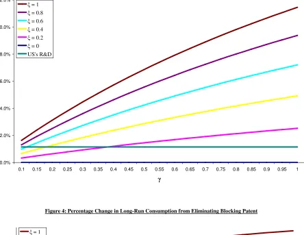
Secondly, increasing patent breadth may be an effective solution to the potential problem of R&D

underinvestment. The resulting positive effect on long-run consumption can be substantial because the

harmful effects of dynamic and static distortions are relatively insignificant. However, the damaging

effect of blocking patent arising from socially suboptimal profit-sharing arrangements between

patentholders can be quantitatively significant. Thirdly, the dynamic distortionary effect on capital

accumulation has a more severe impact on consumption than the static distortionary effect from markup

pricing unless the fraction of competitive industries in the economy is very large. Finally, it considers the

effect on consumption during the transition dynamics. In particular, the economy does not always

experience a significant fall in consumption in response to the increase in patent protection. Over a wide

range of parameters, upon the strengthening of patent protection, consumption gradually rises towards the

new balanced growth path by reducing physical investment and temporarily running down the capital

stock. This finding contrasts that of Kwan and Lai (2003), whose model does not feature capital

accumulation and hence predicts consumption losses during the transition path.

This paper relates to a number of studies. It provides an explanation and a potential solution to the

R&D underinvestment problem identified by Jones and Williams (1998) and (2000). Jones and Williams

(1998) develop a method to calculate the social rate of return to R&D based on endogenous-growth

theory and show that estimates from the empirical productivity literature represent lower bounds on the

true social rate of return. Using this information, they find that the socially optimal amount of R&D

investment is at least two to four times larger than the actual amount. Jones and Williams (2000) adopt a

conclusion that there is underinvestment in R&D over a wide range of parameters.3 The current paper follows this latter approach by calibrating a generalized quality-ladder growth model with patent breadth

as a policy instrument to show that the R&D underinvestment problem arises from insufficient patent

breadth, and increasing patent breadth may be an effective solution to this problem. Furthermore, the

calibration exercise takes into consideration Comin’s (2004) critique that long-run TFP growth may not

be solely driven by R&D.

In terms of qualitative analysis, it complements the patent-design literature,4 which is mostly based on a partial-equilibrium setting, in providing a general-equilibrium analysis on optimal patent

breadth and in identifying an important dynamic distortion on capital accumulation. O’Donoghue and

Zweimuller (2004) is the first study that merges the patent-design and endogenous growth literatures to

analyze the effects of patentability requirement, lagging and leading breadth on economic growth in a

simple quality-ladder growth model. However, their focus was neither in characterizing the optimal patent

breadth nor in quantifying the effects of eliminating blocking patent and increasing patent breadth. In

addition, the current paper generalizes their model in a number of dimensions. For example, the usual

Cobb-Douglas aggregator for intermediate goods is generalized to a CES aggregator to derive the

condition under which patent breadth becomes ineffective in stimulating R&D. Goh and Olivier (2002)

analyze the welfare effects of patent breadth in a two-sector variety-expanding growth model, and

Grossman and Lai (2004) analyze the welfare effects of strengthening patent protection in developing

countries as a result of the TRIPS agreement using a multi-country variety-expanding model. However,

these studies do not analyze patent breadth in an environment with sequential innovations. Li (2001)

analyzes the optimal policy mix of R&D subsidy and lagging breadth in a quality-ladder model with

3

Stokey (1995) also calibrates an R&D-growth model to examine the range of parameters under which the market economy underinvests in R&D.

4

endogenous step size, but he does not consider leading breadth. Furthermore, none of the abovementioned

studies feature capital accumulation so that the dynamic distortion is absent.

Laitner (1982) identifies in an exogenous growth model with overlapping generations of

households that the existence of an oligopolistic sector and its resulting pure profits as financial assets

creates both the usual static distortion from markup pricing and an additional dynamic distortion on

capital accumulation due to the crowding out of households’ portfolio space, and he finds that the latter is

more significant than the former. The current paper extends this study to show that this dynamic

distortion also plays an important role and through a different channel in an R&D-driven endogenous

growth model in which both patents and physical capital are owned by households as financial assets.

In terms of quantitative analysis, this paper relates to Kwan and Lai (2003) and Chu (2007).

Kwan and Lai (2003) numerically evaluate the effects of extending the effective lifetime of patent in the

variety-expanding model originating from Romer (1990) and find substantial welfare gains despite the

temporary consumption losses during the transition path in their model. Chu (2007) uses a generalized

variety-expanding model and finds that whether or not an extension in the patent length is effective in

stimulating R&D depends crucially on the patent-value depreciation rate. At the empirical range of

patent-value depreciation rates estimated by previous studies, patent extension has only limited effects on

R&D and thus social welfare. Therefore, Chu (2007) and the current paper together provide a comparison

on the effectiveness of patent length and patent breadth in solving the R&D underinvestment problem.

The crucial difference between these two policy instruments arises because patent length affects future

monopolistic profits while patent breadth affects current monopolistic profits.

The rest of the paper is organized as follows. Section 2 describes the generalized quality-ladder

model and derives the analytical characterization of optimal patent breadth and the dynamic distortion on

capital accumulation. Section 3 calibrates the model and numerically evaluates the effects of eliminating

blocking patent and increasing patent breadth on consumption. The final section concludes with some

2. Optimal Patent Breadth

The patent-design literature has identified and analyzed four patent-policy tools: (a) the term of patent or

simply patent length; (b) patentability requirement; (c) lagging breadth; and (d) leading breadth.5 In a standard quality-ladder growth model, lagging breadth (i.e. patent protection against imitation) is assumed

to be complete while leading breadth (i.e. patent protection against subsequent innovations) is assumed to

be zero. This section derives the second-best optimal level of lagging and leading breadth chosen by a

benevolent government in a generalized quality-ladder growth model.

The model is a generalized version of Grossman and Helpman (1991) and Aghion and Howitt

(1992). To prevent the model from overestimating the social benefits of R&D and hence the extents of

underinvestment in R&D, long-run TFP growth is assumed to be driven by both R&D investment and an

exogenous process as in Comin (2004). To prevent the model from overstating the effectiveness of patent

breadth in stimulating R&D, the usual Cobb-Douglas aggregator for the quality-enhancing intermediate

goods is generalized to a CES aggregator as in Laitner and Stolyarov (2005). To maintain the analytical

tractability of the aggregate conditions under the CES aggregator, all the intermediate-goods industries

are assumed to be monopolistic in this section; consequently, the static distortion is absent. To introduce

the static distortionary effect of markup pricing into the model, a special case of the Cobb-Douglas

aggregator will be considered in addition to the CES aggregator when performing the numerical exercises

in Section 3. Furthermore, computation of the transition dynamics is possible under the Cobb-Douglas

aggregator.6 In order to perform a more realistic calibration, the model is further modified to include physical capital, which is a factor input for the production of intermediate goods and R&D, and the final

goods can be used for consumption or investment in capital. Finally, the class of first-generation

R&D-driven endogenous growth models, such as Grossman and Helpman (1991) and Aghion and Howitt

5

See, e.g. O’Donoghue and Zweimuller (2004) for an overview of these four patent-policy tools. For a more detailed discussion on patentability requirement and leading breadth, refer to O’Donoghue (1998) and O’Donoghue, Scotchmer and Thisse (1998).

6

(1992), exhibits scale effects and is inconsistent with the empirical evidence in Jones (1995a).7 In the present model, scale effects are eliminated by assuming increasing difficulty in R&D successes as in

Segerstrom (1998), which becomes a semi-endogenous growth model.8

The various components of the model are presented in Sections 2.1–2.9, and the balanced-growth

equilibrium is defined in Section 2.10. Section 2.11 derives the first-best social optimum, and Section

2.12 characterizes the second-best optimal level of patent breadth.

2.1. Representative Household

The infinitely-lived representative household maximizes life-time utility that is a function of per-capita

consumption

c

_t of the numeraire final goods and is assumed to have the iso-elastic form given by

(1)

U

e

nt

c

t

dt

σ

σ ρ

−

=

− ∞

− −

1

1 0

) (

.

1 ≥

σ

is the inverse of the elasticity of intertemporal substitution. The household has

L

t

=

L

0exp(

n

.

t

)

members at time t. The population size at time 0 is normalized to one, and n>0 is the exogenous

population growth rate.

ρ

is the subjective discount rate. To ensures that lifetime utility is bounded,

(A1)

ρ

>n.

The household maximizes (1) subject to a sequence of budget constraints given by

(2) at =at(rt −n)+wt −ct.

Each member of the household inelastically supplies one unit of homogenous labor in each period to earn

a real wage income wt. at is the value of risk-free financial assets in the form of patents and physical

7

See, e.g. Jones (1999) for an excellent theoretical analysis on scale effects. 8

capital owned by each household member, and rt is the real rate of return on these assets. The familiar

Euler equation derived from the intertemporal optimization is

(3) ct =ct(rt −

ρ

)/

σ

.

Along the balanced-growth path, ct increases at a constant rate gc. The steady-state real interest rate is

(4) r=

ρ

+gc

σ

.

2.2. Final Goods

This sector is characterized by perfect competition, and the producers take both the output price and input

prices as given. The production function for the final goods Yt is a CES aggregator of a continuum of

differentiated quality-enhancing intermediate goods X_t(j) for j∈[0,1] given by

(5)

ε ε

/ 1 1

0

) (

= X j dj

Yt t ,

where

ε

∈

[

0

,

.

1

)

. The constant elasticity of substitution as well as the absolute value of demand elasticity

is 1/(1−

ε

). This formulation nests the usual Cobb-Douglas aggregator in quality-ladder models as a

special case with

ε

=0. The familiar aggregate price index is ( ) 1

/ ) 1 ( 1

0

) 1 /(

= =

−

−

ε ε ε

ε

dj j P

P_{t t} , and the

demand curve for each variety of intermediate goods is

(6) X_t(j)=P_t(j)−1/(1−ε)Y_t.

2.3. Intermediate Goods

There is a continuum of monopolistic industries producing the differentiated quality-enhancing

who owns the latest R&D-driven technology for production. The production function in each industry j

has constant returns to scale in labor and capital inputs and is given by

(7)

(

)

(

)

1

(

)

, , ) (

j

L

j

K

Z

z

j

X

_t

=

mt j _{t x}α_{t x}−_tα _.

) (

, j

Kxt and Lx,t(j) are respectively the capital and labor inputs for producing intermediate-goods j at

time t. Z_t =Z₀exp(g_Zt) represents an exogenous process of productivity improvement that is common

across all industries and is freely available to all producers. _zmt(j) _{is the industry leader’s level of}

R&D-driven technology, which is increasing over time through R&D investment and successful innovations.

1 >

z is the exogenous step-size of a technological improvement arising from each innovation. m_t(j),

which is an integer, is the number of innovations that has occurred in industry j as of time t. The marginal

cost of production in industry j is

(8)

α α

α

α

−

−

=

1 )

(

1

1

)

(

t t

t j m t

w

R

Z

z

j

MC

t ,

where Rt is the rental price of capital. The optimal price is a constant markup

µ

over the marginal cost

of production given by

(9) Pt(j)=

µ

.MCt(j).

The profit-maximizing markup for an unconstrained monopolist is 1/

ε

. With a Cobb-Douglas

aggregator,

ε

=0; therefore, it is always the closest rival’s marginal cost that is the binding constraint.

Then, in the standard case of complete lagging breadth and zero leading breadth (to be defined in

Sections 2.5 and 2.6), the industry leader is able to charge a markup of z over the marginal cost without

losing its market share to the closest rival. With a CES aggregator,

µ

≡

min{

z

,

.

1

/

ε

}

. If z≥1/

ε

, then

increasing leading breadth would have no stimulating effects on R&D because the industry leader would

always choose a markup of 1/

ε

regardless the level of leading breadth. To analyze the implications of

(A2) z<1/

ε

.9

Then, the amount of profit earned by the leader of industry j at time t is

(10)

π

t(j)=(z−1)MCt(j)Xt(j).

2.4. Patent Breadth

This subsection presents the Bertrand equilibrium price and profit in the presence of patent breadth, which

is denoted by

η

, under the optimal profit-sharing arrangement. Then, in the following two subsections,

η

is decomposed into lagging breadth

η

lag and leading breadth

η

lead (i.e.

η

=

η

lag +

η

lead) to demonstrate

the underlying assumptions behind the following analytically tractable expressions

(11) P_t(j)=zηMC_t(j)

(12) t(j)=(z −1)MCt(j)Xt(j)

η

π

for

η

∈(0,∞) and j∈[0,1]. The expression for the equilibrium price is consistent with the seminal work

of Gilbert and Shapiro’s (1990) interpretation of “breadth as the ability of the patentee to raise price.” A

broader patent breadth corresponds to a larger

η

, and vice versa. Therefore, an increase in patent breadth

enhances the incentives for R&D by raising the amount of monopolistic profit captured by each

innovation but worsens the distortionary effects of markup pricing. This discussion implicitly assumes

that zη <1/

ε

because the markup is now given by

µ

min{ ,.1/

ε

} η z

≡ . When zη =1/

ε

, patent breadth

has no more stimulating effects on R&D and no more distortionary effects from markup-pricing.

2.5. Lagging Breath

The first deviation from standard quality-ladder models is the introduction of incomplete lagging breadth.

Assume zero leading breadth

η

lead =0 as in standard models for now. To reiterate, each innovation is a

9

constant step-size z of a technological improvement, and this production technology, once invented,

becomes public knowledge to fulfill the disclosure requirement for obtaining a patent. In the case of

complete lagging breadth, the patent for mt(j) allows the new industry leader to produce with any

technology level ( m_t(j) 1, m_t(j)] z

z −

∈ , but the profit-maximizing level is _zmt(j)_{. The former industry leader,}

who holds the patent for mt(j)−1, is now also technologically feasible to upgrade its production

process. However, to do so, she would infringe the patent of the new industry leader, and any licensing

agreement would drive the licensee’s profit to zero.

The parameter

η

lag ≤1 represents the degree of lagging breadth. In the special case of complete

lagging breadth

η

lag =1, any technology level beyond

1 ) (j− m_t

z is protected by the patent for mt(j). In

the case of incomplete lagging breadth

η

lag <1, only technology level beyond

lag

t j

m

z ( )−η is protected. The

following diagram illustrates the concept of incomplete lagging breadth.

In other words, although the invention is a quality improvement of z, the patent only protects part of this

invention lag

zη against imitators. Therefore, with incomplete lagging breadth, the Bertrand equilibrium

price becomes

(13)

P

_t

(

j

)

z

ηlag

MC

_t

(

j

)

=

for

η

lag ∈(0,1) and j∈[0,1]. The amount of profit is

(14) t

(

j

)

(

z

1

)

MC

t

(

j

)

X

t

(

j

)

lag

₋

=

η

π

for

η

lag∈(0,1) and j∈[0,1]. Incomplete protection against imitators forces the industry leader to lower

its markup. On one hand, incomplete lagging breadth reduces the distortionary effects of markup pricing;

on the other hand, the reduced profit worsens the incentives for R&D. 1

) (j− m_t

z _zmt(j)

patent protection

lag

t j

m

2.6. Leading Breadth

The second deviation from standard models is the introduction of nonzero leading breadth, which protects

patentholders against subsequent innovators. The formulation of leading breadth originates from

O’Donoghue and Zweimuller (2004). Assume complete lagging breadth

η

lag =1 as in standard models

for now. The degree of leading breadth is represented by

η

lead ∈{0,1,2,...}. Standard models assume zero

leading breadth (i.e.

η

lead =0). For example, if

η

lead =1, then the most recent innovation infringes the

patent of the second-most recent innovator. If

η

lead =2, then the most recent innovation infringes the

patents of the second-most and the third-most recent innovators, etc. The following diagram illustrates the

concept of nonzero leading breadth with an example of leading breadth equal two.

Therefore, nonzero leading breadth facilitates the new industry leader and the previous innovators, whose

patents are infringed, to consolidate market power through licensing agreements resulting in a higher

markup.10 The Bertrand equilibrium price under nonzero leading breadth is

(15) Pt(j) z1 MCt(j)

lead

η

+

=

for

η

lead ∈{1,2,...} and j∈[0,1]. Assumption 1 is sufficient to derive this equilibrium markup price.

Assumption 1: An infringed patentholder cannot become the next industry leader while she is still covered by a licensing agreement in that industry.11

10

See, e.g. Gallini (2002) and O’Donoghue and Zweimuller (2004), for a discussion on market-power consolidation through licensing agreements.

11

The sufficiency of this assumption in determining the markup price is most easily understood with an example. Suppose leading breadth is one and lagging breadth is complete, the lower bound on the profit-maximizing markup is the square of z, which is the limit price from the collusion of the most recent and the second-most recent innovators against the third-most recent innovator, whose patent is not infringed upon by the most recent invention. In this example, the limit-pricing markup would be even larger if the third-most recent innovator happens to be the new industry leader. Continuing this reasoning, the markup could grow without bound or until it equals 1/ε;

) (j m_t

z _zmt(j)+2

patent protection for _zmt(j)

1 ) (j+ m_t

Then, the amount of monopolistic profit generated in each period by the licensing agreement between the

industry leader and the infringed patentholders is

(16) ( ) ( 1 1) ( ) ( )

j X j MC z

j _{t t}

t

lead −

= +η

π

for

η

lead ∈{1,2,...} and j∈[0,1].

Determining the share of profit obtained by the industry leader requires solving the profit-sharing

arrangement (i.e. the terms in the licensing agreement) between patentholders. A stationary outcome is

assumed to simplify the analysis.

Assumption 2:There is a set of stationary profit-sharing arrangements for each η_lead ∈{1,2,...} denoted

by =( ₁ , ₂ ,..., ₁₊lead )∈[0,1]

lead lead

lead

lead η

η η

η

η _{σ σ σ}

σ , where lead

i

η

σ is the share of profit received by the i-th most

recent innovator when leading breadth is η_lead, and 11 =1

+

=lead lead

i i

η _ση

.

Although the shares of profits and licensing fees eventually received by the owner of an invention are

constant overtime, the present value of profits is determined by the actual profit-sharing arrangement. The

two extreme cases are: (a) complete frontloading

σ

ηlead =(1,0,...,0)_{; and (b) complete backloading}

) 1 ,..., 0 , 0 ( =

lead

η

σ

. Complete frontloading maximizes the stimulating effect of leading breadth on R&D

by maximizing the present value of profits. The opposite effect of blocking patent arises when profits are

backloaded, and complete backloading maximizes this damaging effect on the incentives for R&D.

Assumptions 1 and 2 originate from O’Donoghue and Zweimuller (2004) to formalize the

modeling of leading breadth, but they did not derive the equilibrium outcome that requires solving the

bargaining game between patentholders. Instead, this paper characterizes the optimal patent breadth by

deriving the optimal profit-sharing arrangement.

Assumption 3:The patent authority is able to enforce the socially optimal profit-sharing arrangement in the licensing agreements between patentholders.

Proposition 1a: For any given level of patent breadth, the complete frontloading profit-sharing arrangement is socially optimal if there is underinvestment in R&D in the decentralized equilibrium.

Proposition 1b: In the special case of labor being the only factor input for R&D, the complete frontloading profit-sharing arrangement is socially optimal if and only if there is underinvestment in

R&D in the decentralized equilibrium.

Intuitively, the first-order distortionary effect of markup pricing is determined by

η

, independent of the

profit-sharing arrangement between patentholders. Therefore, given a level of patent breadth, the society

is better off by having a profit-sharing arrangement that creates the largest incentives for R&D if there is

underinvestment in R&D in the market economy. However, the underinvestment in R&D is not a

necessary condition when capital is also a factor input for R&D because stimulating the incentives for

R&D in this case also increases the rate of investment in capital that partly offsets the dynamic

distortionary effect of markup pricing on capital accumulation.

Proposition 1 establishes the condition for the social optimality of the complete frontloading

profit-sharing arrangement, in which the infringed patentholders of previous inventions allow the new

industry leader to capture the entire amount of profits from her invention until the next innovation occurs.

Every successful innovator goes through the cycle of being an infringing industry leader initially and an

infringed patentholder subsequently. Therefore, the distinction between the frontloading and backloading

example of this profit-sharing arrangement is a royalty-free cross-licensing agreement.12 From a policy perspective, the complete frontloading profit-sharing arrangement should be implemented by the patent

authority through the following policies: (a) compulsory licensing with an upper limit on the amount of

licensing fees charged to subsequent inventors of more advanced technology; and (b) making

patent-infringement cases in court favorable to subsequent inventors of more advanced technology.

Given Proposition 1, the equilibrium price and the amount of profit for an industry leader are

respectively Pt(j) z MCt(j) η

= and t(j)=(z −1)MCt(j)Xt(j) η

π

. In the case of complete lagging

breadth and zero leading breadth,

η

=1. In the case of incomplete lagging breadth and zero leading

breadth,

η

∈(0,1). In the case of complete lagging breadth and nonzero leading breadth,

η

∈{2,3,...}. In

the general case of incomplete lagging breadth and nonzero leading breadth,

η

∈(0,∞). For example,

5 . 1 =

η

corresponds to lagging breadth of 0.5 and leading breadth of 1.

2.7. Aggregation

The aggregate production function for the final goods is

(17) α α

ε

ε −

=

= 1

, , /

1 1

0

)

( _{t t xt xt}

t

t X j dj AZ K L

Y ,

where

ε ε ε ε

/ ) 1 ( 1

0

) 1 /( ) (

) (

−

−

≡ z dj

A_t mt j _{is the level of R&D-driven technology.}

=

1 0

, ,

K

(

j

)

dj

K

_{xt xt} and

=

1 0

, ,

L

(

j

)

dj

L

xt xt are total labor and capital inputs for production. The market-clearing condition for the

final goods is

(18) Yt =Ct +It.

12

t t

t Lc

C = is the aggregate consumption, and It is the investment in physical capital. The factor

payments for the final goods are

(19) Yt =wtLx,t +RtKx,t +

π

t.

=

1 0

)

(

j

dj

t

t

π

π

is the total amount of monopolistic profits. Substituting (7) and (8) into (12) and then

summing over all industries yields

(20) t Yt

− =

µ

µ

π

1 .

Therefore, the growth rate of monopolistic profits equals the growth rate of output denoted by

g

_Y. The

amount of factor payments for labor and capital inputs are

(21) wtLxt Yt

− =

µ

α

1

, ,

(22) R_tK_xt = Y_t

µ

α

, .

(22) shows that the markup drives a wedge between the marginal product of capital and its rental price.

As will be shown below, this wedge creates a distortion on the rate of investment in physical capital.

Finally, the value of GDP should include the amount of investment in R&D such that

(23) GDP_t =Y_t +w_tL_r,t +R_tK_r,t.13

t r

L_, and Kr,t are respectively the number of workers and the amount of capital for R&D.

2.8. Capital Accumulation

The market-clearing condition for physical capital is

13

(24) Kt =Kx,t +Kr,t.

t

K is the total amount of capital available in the economy at time t. The law of motion for capital is

(25) Kt = It −Kt

δ

δ

is the rate of depreciation. Denote the balanced-growth rate of capital by

g

K; then, the endogenous

steady-state investment rate in physical capital is

(26) i=(g_K +

δ

)K_t /Y_t

for all t. The no-arbitrage condition rt =Rt −

δ

for the holding of capital and (22) imply that the

steady-state capital-output ratio is

(27)

) )( 1

(

δ

µ

α

+ −

=

r s Y

K

K t

t

.

K

s

is the endogenous steady-state share of capital for R&D. Substituting (27) into (26) yields

(28)

+

+

−

=

δ

δ

µ

α

r

g

s

i

K

K

)

1

(

.

In the Romer model, (skilled) labor is the only factor input for R&D (i.e.

s

K

=

0

); therefore, the

distortionary effect of markup pricing on the rate of investment is unambiguously negative (i.e.

0 /∂ <

∂i

µ

). In the current model, there is an opposing positive effect operating through

s

K. Intuitively,

an increase in patent breadth raises the private return on R&D and consequently, the share of capital

employed in the R&D sector. Proposition 2 in Section 2.11 shows that the negative distortionary effect

still dominates if the intermediate-goods sector is at least as capital intensive as the R&D sector.

2.9. R&D

) (j

V_t is the value of the patent owned by the leader in industry j at time t and is determined by the

following no-arbitrage condition

The first terms in the right is the flow profit generated by the patent at time t. The second term is the

capital gain due to the growth in profit. The third term is the expected value of capital loss due to creative

destruction, and

λ

t is the Poisson arrival rate of the next innovation in the same industry. This

no-arbitrage condition can be re-expressed as

(30)

) ( / ) (

) ( )

(

j V j V r

j j

V

t t t t

t t

− + =

λ

π

.

The aggregate value of the patents owned by all the industry leaders at time t is

(31)

t t t t

t t

t

V

V

r

Y

dj

j

V

V

/

1

)

(

1

0

+

−

−

=

=

λ

µ

µ

.

Since the amount of monopolistic profits varies across industries with the CES aggregator, it

leads to strategic considerations in terms of targeting innovations to a particular industry. To avoid this

problem, the following assumption is made.

Assumption 4: Innovation successes of the R&D entrepreneurs are randomly assigned to the industries in the intermediate-goods sector.

Therefore, the steady-state no-arbitrage value of achieving a new successful innovation at time t is the

expected present value of the stream of monopolistic profits given by

(32)

Y t t

g r

Y V

− + − =

λ

µ

µ

1

.14

The arrival rate of an innovation success for an R&D entrepreneur h∈[0,1] is a function of labor input

) (

, h

L_rt and capital input K_r,t(h) given by

(33)

(

)

(

)

1

(

)

, ,

h

L

h

K

h

_{t rt rt}

t

β β

ϕ

λ

−

=

.15

14

t

ϕ

is a productivity parameter that the entrepreneurs take as given. The amount of expected profit from

R&D is

(34) Et[

π

r_,t(h)]=Vt

λ

t(h)−wtLr_,t(h)−RtKr_,t(h).

The first-order conditions are

(35)

−

V

t t

K

rt

h

L

rt

h

=

w

t

β

ϕ

β

)

(

(

)

/

(

))

1

(

_{, ,} ,

(36)

V

t t

K

rt

h

L

rt

h

=

R

t

−1 ,

,

(

)

/

(

))

(

β

ϕ

β

.

To eliminate scale effects and capture various externalities, the individual R&D productivity

parameter

ϕ

_t at time t is assumed to be decreasing in the level of R&D-driven technology A_t such that

(37) _φ

γ β β

ϕ

ϕ

₋

− −

= ₁

1 1

,

, )

(

t t r t r t

A L K

,

where

=

1 0

, ,

K

(

h

)

dh

K

rt rt and

=

1 0

, ,

L

(

h

)

dh

L

rt rt .

γ

∈(0,1] captures the intratemporal negative

congestion or duplication externality or the so-called “stepping on toes” effects, and

φ

∈(−∞,1) captures

the externality of intertemporal knowledge spillovers.16 Given that the arrival of innovations follows a Poisson process, Laitner and Stolyarov (2005) appeal to the Law of Large Numbers to show that the

aggregate technology can be re-expressed as At

(

.z( ).t

)

~

exp

λ

ε

= , where ~(

ε

)≡( ε/(1−ε) −1)(1−

ε

)/

ε

z

z .

Therefore, the law of motion for R&D-driven technology along the balanced-growth path, in which

λ

is

constant, is given by

(38) .

~

(

)

~

(

)

(

)

.

~

(

)

1 , , 1

,

,

ε

ϕ

ε

ϕ

ε

λ

β β φ β β γ

z

L

K

A

z

L

K

A

z

A

A

_t

=

_t

=

_{t t rt r}−_t

=

_{t rt r}−_t .

15

This specification nests the “knowledge-driven” specification in Romer (1990) as a special case with β =0 and the “lab equipment” specification in River-Batiz and Romer (1991) as a special case with β =α.

16

This specification captures how semi-endogenous growth models eliminate scale effects as in Jones (1995b). )

1 , 0 (

∈

φ corresponds to the “standing on shoulder” effect, in which the economy-wide R&D productivity A_qϕ

Along the balanced-growth path, the growth rate of R&D-driven technology denoted by

g

A is related to

the population growth rate such that

(39)

z

g

n

A

L

K

A

A

g

_K

t t r t r

t t A

−

−

+

−

=

=

=

₋

−

φ

β

γ

φ

β

γ

ε

ϕ

φ

γ β β

1

)

1

(

1

)

(

~

)

(

. . .

1 1

, ,

.

Then, the steady-state rate of creative destruction is

λ

=

g

_A

/

~

z

(

ε

)

.

2.10. Balanced-Growth Equilibrium

The analysis starts at t =0 when the economy has reached its balanced-growth path corresponding to the

patent policy {

η

}. The equilibrium is a sequence of prices {wt,rt,Rt,Pt(j),Vt}∞t₌₀ and a sequence of

allocations

{

a

t

,

c

t

,

I

t

,

Y

t

,

X

t

(

j

),

K

x,t

(

j

),

L

x,t

(

j

),

K

r,t

(

h

),

L

r,t

(

h

),

K

t

,

L

t

}

∞t=0 that are consistent with the

initial conditions {K₀,L₀,Z₀,A₀,

ϕ

₀} and their subsequent laws of motions. Also, in each period,

(a) the representative household chooses {at,ct} to maximize utility taking {wt,rt} as given;

(b) the competitive firms in final-goods sector choose {Xt(j)} to maximize profits according to the

production function taking {Pt(j)} as given;

(c) the industry leaders j∈[0,1] in the intermediate-goods sector choose {Pt(j),Kx_,t(j),Lx_,t(j)}

to maximize profits according to the Bertrand price competition and the production function

taking {R_t,w_t} as given;

(d) the entrepreneurs h∈[0,1] in the R&D sector choose {K_r,t(h),L_r,t(h)} to maximize profits

according to the R&D production function taking {

ϕ

t,Vt,Rt,wt} as given;

(e) the market for the final-goods clears such that Yt =Ct +It;

(f) the full employment of capital such that Kt =Kx,t +Kr,t; and

Equating the first-order conditions (21) and (35) and imposing the balanced-growth condition

(40) 1 _,

~

(

)

,

ε

ϕ

β β

z

K

L

g

_A

=

_{t r}−_{t rt}

yield the steady-state R&D share of labor inputs given by

(41)

−

+

−

−

−

=

−

L Y

L

g

r

s

s

λ

λ

µ

α

β

(

1

)

1

1

1

.

Similarly, solving (22), (36) and (40) yields the steady-state R&D share of capital inputs given by

(42)

−

+

−

=

−

K Y

K

g

r

s

s

λ

λ

µ

α

β

(

1

)

1

.

The balanced-growth rates of various variables are given as follows. Given that the steady-state

investment rate is constant, the steady-state growth rate of per capita consumption is

(43) g_c =g_Y −n.

From the aggregate production function (17), the steady-state growth rates of output and capital are

(44)

g

Y

=

g

K

=

n

+

(

g

A

+

g

Z

)

/(

1

−

α

)

.

Using (39) and (44), the steady-state growth rate of R&D-driven technology is determined by the

exogenous population growth rate

n

and productivity growth rate

g

Z given by

(45)

− + −

− − =

−

Z

A n g

g

α

β

α

β

γ

φ

1 1

1 1

.

Long-run TFP growth denoted by

g

TFP

≡

g

A

+

g

Z is empirically observed. For a given

g

TFP, a higher

value of

g

_Z implies a lower value of

g

_A as well as a lower calibrated value for

γ

/(1−

φ

) indicating

smaller social benefits from R&D.

2.11. First-Best Social Optimum

To derive the socially optimal equilibrium rate of investment i* and R&D shares of labor s*L and capital

*

K

(46) ∞ − − −

−

−

=

0 1 ) (

1

)

/

)

1

((

dt

L

Y

i

e

U

nt t t

σ

σ ρ

subject to: (a) the aggregate production function expressed in terms of

s

L and

s

K given by

(47) = − α − 1−α α 1−α

) 1 ( ) 1

( K L t t

t t

t AZ s s K L

Y ;

(b) the law of motion for capital expressed in terms of i given by

(48) Kt =iYt −Kt

δ

;

and (c) the law of motion for R&D-driven technology expressed in terms of

s

_L and

s

_K given by

(49) ( ) ( ) .~( )

) 1 ( )

1

( β γ βγ β γ

_ϕ

_ε

βγ φ z L K s s A

A_t = _{t K L} − _{t t}− .

After solving this maximization problem, the modified Golden-rule rate of investment is

(50)

δ

σ

ρ

δ

φ

σ

ρ

γ

β

α

+

+

+

−

+

−

+

−

+

=

c K A c A

g

g

g

g

n

g

i

)

1

(

)

1

(

. * .

Proposition 2 provides the condition under which the markup-pricing distortion moves the market

equilibrium rate of investment i away from the social optimum i*.

Proposition 2a: The decentralized equilibrium rate of investment is below the socially optimal investment rate if either there is underinvestment in R&D or labor is the only factor input for R&D.

Proposition 2b: An increase in patent breadth leads to a reduction in the decentralized equilibrium rate of investment if the intermediate-goods sector is at least as capital intensive as the R&D sector.

Similarly, the socially optimal R&D shares of labor s*_L and capital s*_K are respectively

(51) L L c A c A L L

s

s

g

n

g

g

n

g

s

s

−

=

+

−

+

−

−

−

−

≠

−

+

−

+

−

−

−

=

−

(

1

)

1

(52)

K K

c A

c A

K K

s

s

g

n

g

g

n

g

s

s

−

=

+

−

+

−

−

≠

−

+

−

+

−

=

−

(

1

)

1

)

1

(

)

1

(

)

1

(

1

.

* *

λ

σ

ρ

λ

µ

α

β

φ

σ

ρ

γ

α

β

.

(51) and (52) indicate the various sources of externalities and distortion: (a) the negative congestion

externality

γ

∈(0,1]; (b) the positive or negative externality in intertemporal knowledge spillovers

) 1 , (−∞ ∈

φ

; (c) the static surplus appropriability problem (

µ

−1)/

µ

∈(0,1], which is a positive

externality; (d) the distortion of patent protection in driving a wedge of

µ

>1 between the factor payment

for production inputs and their marginal products; and (e) the positive externality of creative destruction

together with the negative externality of the business-stealing effect given by the difference between

) )

1 (

/(

ρ

σ

λ

λ

−n+ − gc + and gA/(

ρ

−n+(

σ

−1)gc +gA). In addition, in the case of suboptimal

profit-sharing arrangements between patentholders, both

s

L

/(

1

−

s

L

)

and

s

K

/(

1

−

s

K

)

are decreased by

the backloading discount factor that is a non-decreasing function of leading breadth.17 Given the existence of positive and negative externalities, it requires a numerical calibration to the data that will be performed

in Section 3 to determine whether the market economy over- or under-invests in R&D.

If the market economy underinvests in R&D as also suggested by Jones and Williams (1998) and

(2000), the government can increase patent breadth to reduce the extent of market failures. However, as

Propositions 2 demonstrates, an increase in

η

mitigates the problem of underinvestment in R&D at the

cost of worsening the dynamic distortion on capital accumulation. At the constrained social optimum, the

government balances these two effects or until patent breadth loses its effectiveness when η _=1/

ε

z .

2.12. Second-Best Optimal Patent Breadth

Given the market equilibrium conditions for i(

η

),

s

L

(

η

)

and

s

K

(

η

)

, the benevolent government

chooses the second-best optimal level of patent breadth

η

* by maximizing

17

(53)

∞ −

− −

−

=

0

1 ) (

1

)

(

dt

c

e

U

nt t

σ

η

σ ρ

subject to the aggregate production function, the law of motion for capital, and the law of motion for

R&D-driven technology. An increase in patent breadth reduces i(

η

) while increases

s

L

(

η

)

and

s

K

(

η

)

.

If an interior solution such that zη* ≤1/

ε

exists, then the first-order condition that balances the opposing

effects on social welfare is given by

(*)

(

)

(

)

(

)

(

)

(

)

(

)

0

* *

* *

* *

=

∂

∂

+

∂

∂

+

∂

∂

η

η

η

ω

η

η

η

ω

η

η

η

ω

L

L K

K I

s

s

i

.

Each of the

ω

.’s represents a weight on the social planner’s optimal rule for patent breadth,

18

and the

value of each

ω

. is increasing in the difference between the socially optimal and the market-equilibrium

levels of its corresponding variable. For example, the further away the market-equilibrium rate of

investment is from its social optimum, the larger the weight the social planner should place on ∂i/∂

η

to

prevent patent breadth from increasing the wedge.

Proposition 3: Suppose there is underinvestment in R&D in the decentralized equilibrium. The first-order condition that characterizes the optimal patent breadth is given by (*) if the patent authority

enforces the socially optimal profit-sharing arrangement between patentholders.

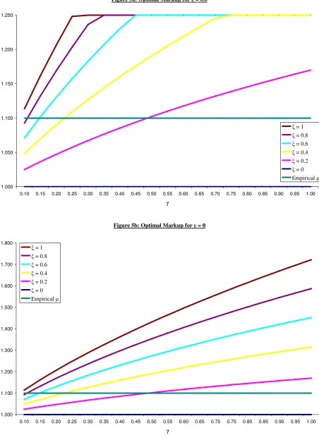
3. Calibration

Using the framework developed above, this section provides a quantitative assessment on the effects of

eliminating blocking patent and increasing patent breadth. Given the recent policy changes in increasing

patent breadth in the 80’s, the structural parameters are calibrated using long-run aggregate data of the

US’s economy from 1953 to 1980. The first numerical exercise considers the effects of eliminating

blocking patent on R&D and consumption. The second numerical exercise considers the effects of

18

increasing patent breadth to the second-best optimum while holding the effect of blocking patent constant.

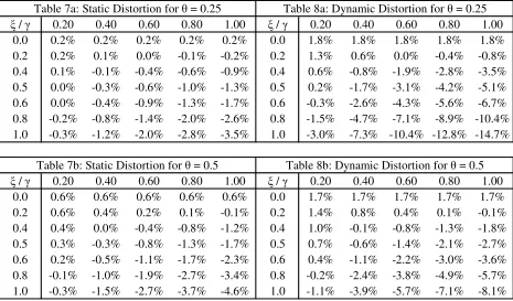
The results for this exercise are firstly presented for the case in which all sectors are monopolistic and

hence the static distortion is absent. Then, the results are presented for the case in which there exist both

monopolistic and competitive sectors in order to introduce static distortion into the model and to compare

the relative magnitude of the static and dynamic distortionary effects. Finally, the transition dynamics are

computed to investigate the effect on consumption during the transitional periods.

3.1. Externality Parameters

The first step is to calibrate the key externality parameters

γ

(intratemporal duplication) and

φ

(intertemporal spillover). For each value of

g

_A,

g

_Z,

n

,

α

and

β

, the balanced-growth condition (45)

determines a unique value for

γ

/(1−

φ

). The annual average TFP growth rate

g

TFP is 1.33%,

19

and the

labor-force growth rate

n

is 1.94%.20 The capital-intensity parameter

α

in the production sector is set to a conventional value of 0.3, and different plausible values for the R&D capital-intensity parameter

} 3 , 2 , , 0

{

α

α

α

β

∈ are considered.

β

=0 corresponds to the knowledge-driven specification in Romer

(1990), and

β

=

α

corresponds to the lab-equipment specification in Rivera-Batiz and Romer (1991) and

Jones and Williams (2000).

β

∈{2

α

,3

α

} corresponds to the case in which the R&D sector is more

capital intensive than the production sector. I will firstly consider the case in which long-run TFP growth

is solely driven by R&D (i.e.

g

TFP

=

g

A and

g

Z

=

0

). Given the above parameters, I firstly calculate the

implied value for

γ

/(1−

φ

), which is sufficient to determine the new balanced-growth level of

consumption. However, holding

γ

/(1−

φ

) constant, a larger

γ

implies a faster convergence rate to the

new balanced-growth path; therefore, it is important to consider different values of

γ

. The calibrated

values of

φ

that correspond to a range of values for

γ

∈[0.1,.1.0] are listed in Table 1.

19

Multifactor productivity for the private non-farm business sector is obtained from the Bureau of Labor Statistics. 20

/ 0.1 0.2 0.3 0.4 0.5 0.6 0.7 0.8 0.9 1.0

0 0.85 0.71 0.56 0.42 0.27 0.12 -0.02 -0.17 -0.31 -0.46

0.81 0.62 0.43 0.24 0.06 -0.13 -0.32 -0.51 -0.70 -0.89

2 0.77 0.54 0.30 0.07 -0.16 -0.39 -0.62 -0.85 -1.09 -1.32

[image:28.612.110.502.71.162.2]

3 0.73 0.45 0.18 -0.10 -0.37 -0.65 -0.92 -1.20 -1.47 -1.75 Table 1: Calibrated Values for

3.2. First-Best Level of R&D Spending

The second step is to calculate the first-best level of R&D spending, which requires the discount rate, the

inverse of the elasticity of intertemporal substitution and the empirical markup. The discount rate is set to

a conventional value of 0.04, and the elasticity of intertemporal substitution (i.e. 1/

σ

) is set to 0.25.21 The implied real interest rate given by

r

=

ρ

+

g

TFP

σ

/(

1

−

α

)

is 11.6%, which is higher than the

historical real rate of return in the US’s stock market, and this higher interest rate implies a lower level of

first-best R&D spending. As a result, the model is less likely to overestimate the extent of R&D

underinvestment. For the empirical markup

µ

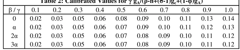
, I make use of Laitner and Stolyarov’s (2004) estimate of

1.10 (i.e. a 10% aggregate markup).22 Given these additional parameters, I firstly calculate the calibrated values for the following useful ratio

γ

.gA/(

ρ

−n+(

σ

−1)gc+(1−

φ

)gA) that appears in (51) and (52)

for a range of values for

γ

∈[0.1,.1.0] and

β

∈{0,

α

,2

α

,3

α

} in Table 2.

/ 0.1 0.2 0.3 0.4 0.5 0.6 0.7 0.8 0.9 1.0

0 0.02 0.03 0.05 0.06 0.08 0.09 0.10 0.11 0.13 0.14

0.02 0.03 0.05 0.06 0.07 0.09 0.10 0.11 0.12 0.13

2 0.02 0.03 0.05 0.06 0.07 0.08 0.09 0.10 0.11 0.12

[image:28.612.105.503.503.587.2]

3 0.02 0.03 0.05 0.06 0.07 0.08 0.09 0.10 0.11 0.12

Table 2: Calibrated Values for gA/( -n+( -1)gc+(1- )gA)

21

It is well-known that there is a discrepancy between the estimated elasticity of intertemporal substitution from dynamic macro models (closed to 1) and econometric studies (closed to 0). Guvenen (2006) shows that this difference is due to the heterogeneity in households’ preferences and wealth inequality. In short, the average investor has a high elasticity of intertemporal substitution while the average consumer has a much lower elasticity. Since my interest is in the effects on consumption, I calibrate the value of according to the average consumer. 22