Environmental test chamber for the support of learning and teaching in intelligent control

Environmental Test Chamber for the Support of

Learning and Teaching in Intelligent Control

C. James Taylor

Engineering Department, Lancaster University, Lancaster LA1 4YR, UK. Email: [email protected]

Key words: Micro-Climate, Ventilation Rate, Multivariable Control, Matlab/Simulink®.

Abstract

1 Introduction

The desire for cost-effective teaching of mechatronics is balanced by the ideal of giving students the opportunity to solve real design problems. Innovations in the use of simulation tools such as MATLAB®/SIMULINK® for teaching signal processing, intelligent control and related subjects may provide low cost options, but can lead to a reduction in the ‘hands-on’ experience for the student.

In this regard, the present paper describes the utility of a low cost, 1m2 by 2m forced ventilation test chamber, for the support of research and teaching in the Engineering Department at Lancaster University. Initially developed for the evaluation of a new ventilation rate controller for agricultural buildings1, the fully instrumented chamber now provides numerous learning opportunities and individual projects, for both undergraduate and postgraduate research students in the Department.

Here, a computer controlled axial fan is positioned at the outlet in order to draw air through the chamber, whilst a ventilation rate sensor measures the associated flow rate. Ventilation rate has been shown to be one of the most significant inputs on the microclimate surrounding plants or animals within the majority of agricultural buildings, including livestock housing, glasshouses and storage warehouses, so good control of this variable is essential2,3,4. A 3-dimensional array of 20 thermocouples, together with a computer controlled heating element positioned at the inlet, completes the basic specifications of the chamber.

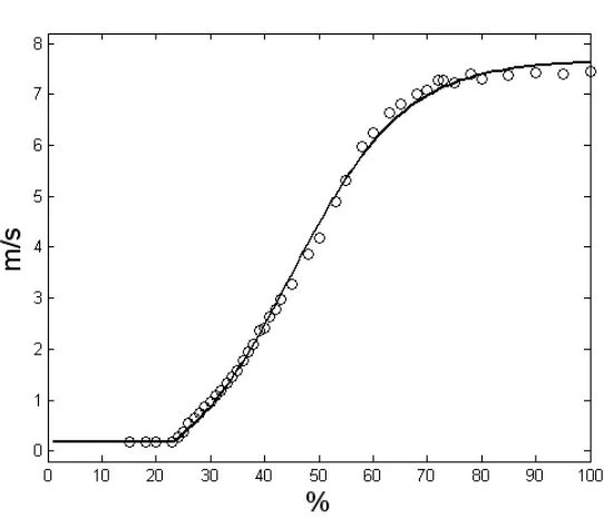
Both variables show evidence of pure time delays and both have a nonlinear gain. For example, at high applied voltages, the steady state airflow rate converges asymptotically to a maximum value determined by the characteristics of the fan. In this manner, the steady state power takes the form of the S-shaped curve illustrated in Fig. 1, requiring some form of adaptive, scheduled or nonlinear control for optimal performance. In this regard, the chamber is presently being utilised to support research into the State Dependent Parameter (SDP) system identification methodology5 and Proportional-Integral-Plus (PIP) control6,7,8.

In addition to this generic research, it is clear that control of the 3-dimensional environment of air-spaces is of increasing interest, with applications in both agriculture and the human built environment, including the automotive industry. In this regard, the chamber allows for research into shifting air flow patterns and incomplete mixing, with the aim of developing an associated distributed multivariable control system for micro-climate.

However, the focus of the present paper is on the chamber’s use as a tool for learning and teaching. With a settling time of ~10 seconds for ventilation rate and ~10 minutes for temperature, open and closed loop experiments are feasible within the timescale of a standard laboratory class. In this regard, the author uses the equipment to support courses in signal processing, intelligent control and MATLAB®/SIMULINK®programming. Furthermore, it has already inspired innovative projects for 3rd / 4th year undergraduate students, as well as postgraduate MSc and PhD students. In supporting the design philosophy of the Department, it provides a valuable modelling and control systems tool, that supersedes existing simulation-based projects in this area.

2 Environmental chamber

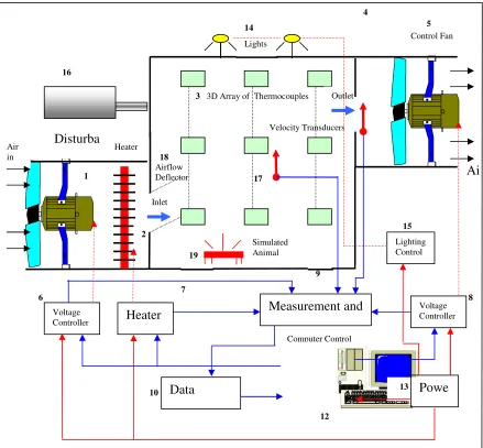
The chamber was designed and constructed by Dr. Phil Leigh1 in 2001,for an initial cost of under £5000, including sensors, software and the accompanying PC. The schematic layout of the chamber is illustrated in Fig. 2, where the numbers [1] – [19] are referred to below.

It consists of a structural aluminium framework in 1m x 1m x 25mm modular sections, with an overall size of 2m (length) x 2m (height) x 1m (width). Twelve 1m x 1m x 5mm rigid perspex sheets are fitted into this framework. Such a modular construction allows for future design flexibility. A circular inlet (0.01327m2) is cut into the lower modular section at one end of the chamber, while a similarly sized outlet is cut into the top modular section at the opposite end.

The outlet has a 320W axial (Vent Axia) fan [5] to draw the air through the chamber. With a diameter of 480mm, a depth of 170mm and an extract capacity of up to 4940 m3/hr it is, in general, suitable for both light and heavy duty use in either ducting or through the wall applications. Such fans are constructed from steel plate with a tough epoxy paint finish, while the impellers are glass filled polyamide for resistance to environmental conditions and abrasive airflow.

Housed within the inlet is a heating element (500w) [2] to warm the airflow drawn into the chamber, together with a second axial fan [1] for generating disturbances to the system. The chamber is bolted together and fastened to a blockboard base on industrial standard casters, which makes the whole installation mobile. For maintenance and installation access purposes, the 1m x 1m panel below the outlet is hinged and can be easily opened. There is a compressible rubber door seal and two catches that tighten the ‘door’ against the main framework to make an airtight seal. The rest of the rig has been sealed with clear flexible silicon to make it as air tight as possible.

both the inlet and outlet in order to record reference input and output temperatures against the internal temperature distribution. These thermocouples are hard-wired to a multiplexer (PCLD-789D) and a PCLD-8115 screw terminal board, which is connected via a DB37 way connector to the Analogue to Digital (AD) PCL-818L board [10] housed in a PC [12].

The outlet airflow rate is measured via an air velocity transducer [4], which has been calibrated against the voltage applied to the axial fan. It is mounted at the centre of the outlet close to the control fan. Both the fans and the heating element are controlled by two Thyristors (type SKKT20B08D, RS Components) that are in turn controlled by a Phase Angle Trigger Module (type SKPC200-240, RS Components) [7, 8, 9]. Again, each circuit is controlled by a PCL-818L (or similar) board.

A second air velocity transducer is positioned inside the 3D-airspace [17]. This can be moved around to record the airflow rate in different areas of the chamber in response to varying ventilator speeds and temperatures. A mechanical means of directing the airflow has been added to allow the airflow to be deflected more precisely where it is required for optimum control [18]. To add more realism to the chamber an internal heat source designed to simulate animal occupancy has been added. This disturbance heat source takes the form of a 60W tubular heater [19], which is controlled manually and mounted on a set of rails, connected via a pulley system to a variable speed, forward and reversible motor.

3 Sensors and control

There are a number of external devices that require interfacing with the microprocessor (PC), including the control fan, disturbance fan and the heating element. The actuators for these devices require an analogue signal, so the digital output from the PC first needs converting to this form. For this purpose a bridging circuit module was designed, with an analogue 0-5 V DC input and a 240 V AC output to the external device to be controlled. This circuit is designed to regulate the AC voltage supplied to the load by a Thyristor pair controlled by a Phase Angle Trigger Module (PATM). The latter is controlled by the analogue 0-5 V DC output from the PCL-818L card inside the PC. Here, various fuses protect the thyristors and PATM module. These components are arranged on an insulating board and housed in a suitable enclosure to ensure mechanical and electrical safety.

This method of AC voltage control from a DC source chops the potential AC voltage sine wave, which limits the amount of voltage that reaches the external device. Thus, by varying the 0-5V DC source via suitable PC software (see below), the speed of the fan or power supply to the heater can be regulated. Such an interfacing method is a form of modulating control. Although alternative on/off or stepwise controllers are cheaper and easier to implement, they can both result in higher fluctuations of the indoor micro-climate when compared to modulating control.

In the case of ventilation rate, for example, stepwise and on/off control are commonly used in countries where feed costs are relatively low, such as the USA. By contrast, modulating control is more prevalent in European countries such as Denmark, Belgium and Holland due to expensive feed costs and more intensive livestock farming. Here, modulating control is used because it provides higher probabilities of a more stable indoor ventilation pattern. This ultimately results in animals consuming less feed to maintain their optimum temperature.

impeller because of its relative ease of use and installation, along with the fact it has a very fast response to differing inputs and can measure low airflow rates to a high degree of accuracy. Additionally, it is very portable and non-intrusive to the airflow and this allows easy measurement of airflow at any point within the 3D airspace.

With regards to temperature, thermocouples are chosen because of their relatively low cost, durability and wide temperature range. Since they rely on the Seebeck effect (the generation of voltage due to the junction of two dissimilar metals under varying temperatures), the thermocouples need special attention when wiring. In particular, terminating the wires creates another thermocouple that requires ‘cold junction’ compensation. The ADAC thermocouples used in the chamber (5508TC, TB5800-TC, and 4012TCEX) correct this natural ‘error’ at the termination panel by offsetting the un-wanted voltage using zener diodes, and by housing these terminations in an isothermal environment.

The output signals from these sensors have to be processed in some way. For example, the output from a thermocouple is a very small voltage, only a few millivolts. Therefore, a signal-conditioning module within the multiplexing board is utilised to convert this tiny voltage into a current signal, amplify it, provide noise rejection, linearisation and cold junction compensation. By contrast, the calibration equations for the sensors, together with any open-loop or feedback control algorithms, are all programmed in software installed on the PC, namely MATLAB®/SIMULINK® and appropriate toolboxes9,10.

Here, an additional Real Time Toolbox10 is essential, since it provides the link to the PC input-output cards. Variables linked into or from the block library subsystems included with this toolbox, connect directly to either the data-logging or actuator channels on the PCL-818L (or similar Analogue to Digital) card.

The exploitation of MATLAB®/SIMULINK® in this manner provides an integrated approach for data processing, time series analysis, graphical presentation of data, control system design, simulation and, finally, control implementation, allowing for a transparent design process ideal for student learning. An initial simulation-based laboratory exercise, such as that described in Section 6, is straightforwardly moved to the real application since the same software environment can be used throughout.

4 Research and student projects

The chamber is particularly useful for the comparative evaluation and refinement of new control methodologies. For example, it is presently being utilised to support research into a novel State Dependent Parameter (SDP) system identification methodology. Here, the nonlinear system is modelled using a quasi-linear model structure in which the parameters vary as functions of the state variables5.

However, the chamber was primarily developed for research on micro-climate control. Here, it is widely recognised that the ventilated airspace in agricultural buildings and the human built environment is imperfectly mixed. Such imperfect mixing leads to gradients in variables such as temperature, humidity, gas, dust and air velocity, all of which affect the micro-environment around the animal or plant. It is clear, therefore, that mathematical models and control systems must adequately account for these nonlinear, imperfect mixing processes. For example, without adequate fresh air supply within a livestock enclosure, animal comfort and welfare are drastically reduced, especially during high density occupation by poultry, pigs or cattle, where excessive levels of moisture, heat and internal gasses are generated.

In practice, pressure disturbances caused by variations in wind speed outside the building have a significant influence on the ventilation rate produced by an axial fan, sometimes resulting in poor indoor micro-environmental conditions. It is not too surprising, therefore, that the lack of effective ventilation rate control is a major cause of production losses and ventilation- related health problems in modern livestock buildings2,3,4.

Recent research using this and similar forced ventilation test chambers have been concerned with the design and implementation of Proportional-Integral-Plus (PIP) control systems8. Here, non-minimal state space (NMSS) models are formulated so that full state variable feedback control can be implemented directly from the measured input and output signals of the controlled process, without resort to the design and implementation of a deterministic state reconstructor or a stochastic Kalman filter6,7.

In contrast to conventional PI/PID controllers, however, PIP design has numerous advantages: in particular, its structure exploits the power of State Variable Feedback (SVF) methods, where the vagaries of manual tuning are replaced by pole assignment or Linear Quadratic (LQ) optimal design6,7. The present author believes that PIP control offers an insightful introduction to modern control theory for students. In particular, the approach provides straightforward access to SVF methods, while avoiding the complication of a Kalman filter. Indeed, a MEng / MSc module in Intelligent Control taught by the author, covers these areas in two days of lectures, utilising the ventilation chamber as a design example throughout.

5 Teaching activities

The chamber is used both to demonstrate key concepts in control theory and as a model for students to solve design problems. Typical subject areas include:

(i) Fig. 1 forms the basis for an open-loop control algorithm, with the appropriate fan voltage for a given ventilation rate obtained directly from the graph. One MATLAB® exercise involves fitting a curve to these steady state operating level data, followed by the implementation of the corresponding open-loop controller using SIMULINK®.

(ii) Of course, the disadvantage of such an open-loop design is its dependence on Fig. 1. This limitation is quickly illustrated by either covering the inlet or using the disturbance fan, in order to represent an external wind disturbance, quickly leading to an off-set in the desired ventilation rate.

(iii) By contrast, a manually tuned closed-loop Proportional-Integral (PI) controller ‘backs-off’ such disturbances and adeptly illustrates the advantages of feedback.

(v) Fig. 1 is also the starting point for a discussion about nonlinear systems and the concept of linearization at an operating point. In particular, the state dependent gain of the system (see Section 6) ensures that the performance of any fixed gain control algorithm will deteriorate when operated away from it’s optimum ventilation rate.

(vi) For small perturbations close to a specified operating point, the open-loop system provides a classical 1st and 2nd order linear response, for the case of ventilation rate and temperature respectively. Such responses may be utilised for the measurement of the gain, time constant, settling time and similar measures of system behaviour.

(vii) It is straightforward to develop a PID-type control algorithm for either variable, using conventional methods such as Ziegler-Nichols. However, the robustness of the final algorithm proves rather poor and the control parameters generally require further optimisation by trial and error. By contrast, the modern model-based approach discussed below, yields robust control for a wide range of operating conditions.

(viii) Since useful experimental data may be collected in just a few minutes, the chamber provides an ideal laboratory-based example for illustrating a data-based approach to system identification. Such models relate the input and output variables in the simplest possible manner, without regard to the internal mechanisms or state variables: e.g. a discrete- or continuous- time transfer function model obtained from a Least Squares based statistical analysis.

6 Worked example

In order to identify the dominant dynamics of the main fan, airflow data are collected for 5% step changes in the applied voltage. In this case, the analysis suggests that the following first order linear difference equation with 2 samples time delay provides the best explanation of the data across a wide range of operating conditions,

) 2 ( ) 1 ( )

(k ₌₋ay k_{− +}bu k₋

y (1)

where y(k) is the air velocity (m/s) and u(k) is the applied voltage expressed as a percentage. Equation (1) is based on a sampling rate of 2 seconds. For example, at low ventilation rates,

743 . 0 − =

a and b₌0.027, so that the Transfer Function (TF) representation of the model is,

) ( 743 . 0 1 027 . 0 ) ( 1 ) ( 1 2 1 2 k u z z k u az bz k y − − − − − = + = (2)

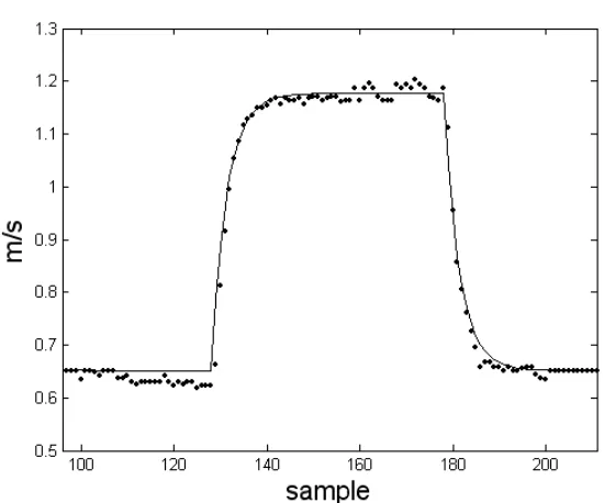
where z−1 is the backward shift operator, i.e., z−iy(k)₌ y(k₋i). In this case, the Coefficient of Determination R_T2 ₌0.9938, implying that over 99% of the variation observed in the data is explained by the model (2), as illustrated by Fig. 4. One advantage of such a transfer function model is its simplicity and ability to characterise the dominant modal behaviour of a dynamic system, making it ideal for control system design. Indeed, the present example demonstrates how, for small perturbations about an operating point, a very simple data-based model can capture almost all of the dynamics of a complex nonlinear system.

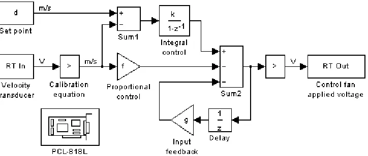
Instead, consider the design of a fixed gain PIP algorithm. Following the approach described by e.g. Ref. [6] – [8], equation (2) is written in a non-minimal state space form and the control gains are optimised using state variable feedback methods. In conventional block diagram terms, the final control system can be implemented as shown in Fig. 3. Here, it is clear that PIP control can be considered as one particular extension of the ubiquitous PI controller, in which the PI action is enhanced by the additional feedback compensator g_⋅u(k₋1).

For clarity, Fig. 3 shows PIP control implemented in its simplest feedback form. In practice, however, the algorithm is usually implemented in an alternative incremental form that avoids the problem of integral-wind up8. It is also important to note that Fig. 3 is derived from the particular model structure given by equation (2). For a generalised transfer function model, the PIP closed loop system is enhanced by higher order forward path and feedback compensators, depending on the order of the model, numerator dimension and number of pure time delays6,7,8. This ensures that the final system is controllable for a general model.

The state space formulation mentioned above, while ideal for solving systems of any dimension, is not strictly necessary for the low order example considered here. Indeed, by assuming the system is exactly represented by (2), standard rules of block diagram analysis can be utilised in a class exercise, to find the closed loop transfer function from Fig. 3, i.e.,

) ( ) ( ) ( ) 1 ( 1 ) ( 3 2 1 2 k d z ga fb z kb a g ga fb z a g kbz k y − − − − − − + + − − + + − + + = (3)

where f, g and k are the proportional, input feedback and integral gains respectively, while )

(k

d is the desired ventilation rate or set point (m/s). By taking the characteristic equation,

0 ) ( ) ( ) 1 (

1₊ g₊a₋ z−1₊ fb₊ga₋g₋a₊kb z−2_{+ −}fb₋ga z−3 ₌ (3)

The control algorithm determined above may be evaluated in both time and frequency domains by taking advantage of Monte Carlo (MC) analysis, which utilises estimates of the parametric uncertainty obtained from the identification algorithm. Here, the model parameters for each realisation in the analysis, are selected randomly from the joint probability distribution defined by the parametric covariance matrix11; and the sensitivity of the PIP controlled system to parametric uncertainty is evaluated from the ensemble of resulting closed loop response characteristics7. For instance, plots of the closed loop step, impulse and frequency responses; and plots of the closed loop pole positions or stochastic root loci.

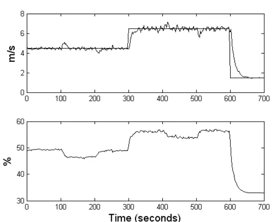
Finally, it is straightforward to implement the algorithm using SIMULINK® as shown by Fig. 3. In this case, typical results from the chamber are illustrated in Fig. 6. Here, the disturbance fan is activated (in the form of a step input) at samples 100, 200, 400 and 500, yielding only a small temporary deviation from the set point in each case, demonstrating the advantage of robust automatic feedback control. The lower subplot of Fig. 6 shows the associated control input signal responding to these disturbances and other stochastic effects.

7 Conclusion

Acknowledgements

The author is grateful to Dr. Phil Leigh1, Dr. Arun Chotai and Prof. Peter Young, all of the Environmental Science Department, Lancaster University, for the design and construction of the test chamber. The research described in this paper is supported by the Engineering and Physical Sciences Research Council.

References

1 P.A. Leigh, ‘Modelling and Control of Micro-Environmental Systems’, PhD thesis (Institute of Environmental and Natural Sciences, Lancaster University, 2002).

2 E. Vranken, ‘Analysis and Optimisation of Ventilation Control in Livestock Buildings’, PhD Thesis (Katholieke Universiteit Leuven, 1999).

3 A.J. Hebner, C.R. Boon and G.H. Peugh, ‘Air patterns and turbulence in an experimental livestock building’, Journal of Agricultural Engineering Research, 64, 209-226 (1996). 4 J.F. Kreider and A. Rabl, ‘Heating, ventilation and air conditioning control systems’,

Heating and cooling of buildings. Design for efficiency (McGraw-Hill Book Co, Singapore, 1996), pp.605-667.

5 P.C. Young, ‘Stochastic, dynamic modelling and signal processing: time variable and state dependent parameter estimation’, in W.J. Fitzgerald et al. (Eds.) Nonlinear and nonstationary signal processing (Cambridge University Press, Cambridge, 2000), pp. 74-114.

6 P.C. Young, M.A. Behzadi, C.L.Wang and A. Chotai, ‘Direct Digital and Adaptive Control by input-output, state variable feedback pole assignment’, International Journal of Control, 46, 867-1881 (1987).

8 C.J. Taylor, P. Leigh, L. Price, P.C. Young, D. Berckmans, K. Janssens, E. Vranken and R. Gevers, ‘Proportional-Integral-Plus (PIP) control of ventilation rate in agricultural buildings’, Control Engineering Practice, 12, 225-233 (2004).

9 The Mathworks, ‘Matlab, Version 6.1’, www.mathworks.com (2001).

10 Humusoft s.r.o., ‘Real Time Toolbox, Version 3.10. Simulink Extension, Version 3.10’, www.humusoft.com (2001).

Figure Captions

Fig. 1 Power curve showing the relationship between applied voltage to the control fan (%) and the steady state ventilation rate (m/s). A flexible logistic growth function has been fitted in a Least Squares sense to better illustrate the relationship between these variables.

Fig. 2 Schematic layout of the micro-environment chamber1. The numbers [1] – [19] are referred to in the text.

Fig. 3 SIMULINK®diagram for on-line PIP control of ventilation rate. The ‘RT In’ and ‘RT Out’ blocks link to the PCL-818L card in the PC.

Fig. 4 Small perturbation experiment based on steps in the applied voltage between 27% and 32%. Airflow velocity (dots) and linear model response (solid trace) plotted against sample number.

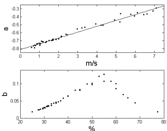
Fig. 5 Estimated parameters for the model (1). Top: a plotted against ventilation rate (m/s) with fitted straight line. Bottom: b plotted against fan voltage (%)

Fig. 1 Power curve showing the relationship between applied voltage to the control fan (%) and the steady state ventilation rate (m/s). A flexible logistic growth

Fig. 2 Schematic layout of the micro-environment chamber1. The numbers [1] – [19] are referred to in the text.

Ai 19 Disturba Simulated Animal 18 Airflow Deflector 4 17 Velocity Transducers 16 15

3 3D Array of Thermocouples

5 Air in 13 12 10 9

6 7 8

Fig. 4 Small perturbation experiment based on steps in the applied voltage between 27% and 32%. Airflow velocity (dots) and linear model response (solid trace)

Fig. 6 PIP control of ventilation rate with various step changes in the applied voltage to the disturbance fan at 100, 200, 400 and 500 seconds. Top: ventilation rate (m/s) and set point.