Modeling Delay and Noise in Arbitrarily
Coupled
RC
Trees
Dinesh Pamunuwa,
Member, IEEE
, Shauki Elassaad, and Hannu Tenhunen
Abstract—Closed-form equations for second-order transfer functions of general arbitrarily coupled resistance–capacitance (RC) trees with multiple drivers are reported. The models allow precise delay and noise calculations for systems of coupled inter-connects with guaranteed stability and represent the minimum complexity associated with this class of circuits. Their accuracy is extensively compared against other relevant models and is found to be better or comparable to more expensive models. All results are derived from a theoretical approach, and their physical basis is examined. The simplicity, accuracy, and generality of the mod-els make them suitable for use in early signal integrity analyses of complex systems and incremental physical optimization.
Index Terms—Crosstalk, delay and noise modeling in VLSI circuits, interconnect modeling, timing analysis, transfer function.
I. INTRODUCTION
I
MPROVEMENTS in lithography have seen continuously shrinking line widths and increasing die sizes, resulting in unprecedented opportunities to implement entire systems on a single chip. This trend of decreasing feature sizes can be ex-pected to continue for the next 8–10 years [1]. With decreasing gate delays and increasing wiring density, noise modeling and its impact on performance and functionality has become very important. The majority of signal wires are typically lossy, and higher aspect ratios to control the resistance result in increased capacitive coupling. This, together with smaller signal rise times, results in heavy crosstalk, which couples a noise voltage onto the victim net. A distinction is usually made between the coupled noise amplitude and the effect of noise on delay. The former can cause functional failures by causing the voltage to swing above or below the logic threshold, while the latter has an impact on the cycle time.The ability to put billions of transistors on a single die has also imposed severe restrictions on the computational com-plexity of noise and delay models used in an iterative design flow. While more accurate modeling is necessary, the sheer
Manuscript received December 6, 2003; revised May 21, 2004 and October 14, 2004. This work was funded partly by Cadence Design Systems, and partly by the Swedish governmental funding agencies Sida, Vinnova, and Exsite. The bulk of this work was carried out when D. Pamunuwa was a graduate intern at Cadence Berkeley Laboratories, Cadence Design Systems, Berkeley, CA 94704 USA. This paper was recommended by Associate Editor D. Blaauw.
D. Pamunuwa is with the Centre for Microsystems Engineering, Depart-ment of Engineering, Faculty of Applied Sciences, University of Lancaster, Lancaster LA14YW, U.K.
S. Elassaad is with the Rio Design Automation, Santa Clara, CA 95054-1137 USA.
H. Tenhunen is with the Laboratory of Electronics and Computer Systems, Department of Microelectronics and Information Technology, Royal Institute of Technology (KTH), Stockholm, SE 16440, Sweden.
Digital Object Identifier 10.1109/TCAD.2005.852279
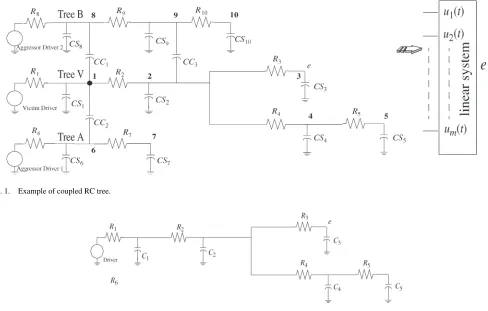
size of the systems prohibits expensive dynamic simulation. Consequently, the subject of delay and noise modeling for very large scale integration (VLSI) circuits has received a vast amount of attention in the literature. The three attributes of accuracy, computational simplicity, and generality are, how-ever, difficult to encompass in a single integrated model. Most reported models that consider the effect of crosstalk on noise and delay either use heuristics that are tailored for specific topologies or use multiple moments that make them expensive. In particular, there is a huge need for an efficient model that can be used in the inner loop of place-and-route algorithms for global signal planning and incremental physical optimiza-tion in circuits with heavy coupling. In addioptimiza-tion to minimal computational complexity, some other specific characteristics are necessary in such a model; it should allow a one-to-one correspondence between the physical structure being modeled, and the electrical circuit being analyzed, so that changes can be quickly and efficiently incorporated, and it should also exhibit fidelity. In incremental physical optimization, the absolute ac-curacy of the delay at any given node predicted by the metric is of secondary importance to the generation of a solution that is the same, or as close as possible, to the solution that would be generated by using a much more accurate delay metric. The Elmore delay [10] possesses this attribute of fidelity, which, coupled with its peerless efficiency, is why it has been and still is very popular in place-and-route algorithms. How-ever, in the face of heavy coupling, its usefulness diminishes, fundamentally because it can only address grounded capacitors. The contribution of this paper is as follows. Closed-form models for generating second-order transfer functions from each driver to the receiver in arbitrarily coupled resistance– capacitance (RC) trees (such as that shown in Fig. 1) repre-senting the minimum complexity for this class of circuits were recently reported [2], [3]. The summation of all waveforms results in the complete response to all switching events at the node of interest, with no restriction on arrival times, and allows both delay and noise estimations. These models are intended for global signal planning, and incremental physical optimization in CAD algorithms. In this paper, the model and constituent expressions are derived from first principles, and formal proofs provided; also, statistical data of extensive comparisons against other relevant models are included. It is also clearly shown how this model saves at least two full tree traversals over the second-order model that bears the closest resemblance to it, while providing comparable accuracy.
This manuscript is organized as follows. The next section presents a detailed overview of the current work that puts the contribution of the reported model in context. Section III
Fig. 1. Example of coupled RC tree.
Fig. 2. Example of simple RC tree.
explains the proposed modeling in detail, which is based on the moments of the circuit, and follows a strict theoretical ap-proach. The proposal for guaranteeing stability and its physical ramifications, and the computational complexity of the models are discussed. Next, the results of running the proposed models on numerous test circuits are presented. The paper ends with a discussion.
II. BACKGROUND
An accurate analysis of signal propagation in interconnects requires solving Maxwell’s equations in three dimensions, which is prohibitively expensive in terms of computation time. However, it is possible to use simplified models in most cases to capture the important effects in the regime of interest [5], [6]. A particular concern with falling rise times is how important inductive effects are, and when and how they should be modeled. A growing body of literature that addresses this issue now exists [7]–[9]. They propose metrics that relate the physical dimensions of the wire to the signal rise time by assuming transverse-electromagnetic (TEM) propagation to de-termine when neglecting inductive effects results in significant errors. The general consensus now is that modeling inductance is necessary for special nets such as clock and power lines, and that the majority of signal lines can be accurately modeled by networks of resistors and capacitors, even with very small rise times. It is important, however, to consider the effect of capacitive crosstalk, which is exacerbated by sharper slew rates. In this paper, interconnects that can be modeled by coupledRC lines are considered.
A. Delay Modeling
Timing analysis in VLSI circuits has long been carried out using the simplified model of anRCtree where all capacitors are connected to ground, whose circuit model is called a simple tree (Fig. 2). There is a large body of literature that deals with delay modeling in simple trees. One of the most important and widely used metrics, the first moment of the impulse response, was proposed back in 1948 as an upper bound for the delay in valve circuits [10] and is known as the Elmore delay. Its attrac-tion is that it uses minimum informaattrac-tion and has unmatched algorithmic simplicity and elegance, explicitly matches the circuit elements to the delay, and yet exhibits good fidelity, giving results as good as more expensive models when used in interconnect optimization algorithms. However, as mentioned, it becomes less accurate as heavy coupling comes into play, and noise waveforms cannot be modeled, as a minimum of two time constants are required to model a voltage spike. Bounds and metrics that give an indication of when the Elmore delay is a poor approximation were developed in [11].
which typically requires2q moments for aqth-order approx-imation, and though very efficient, are too expensive for in-cremental physical optimization. Other estimators based on the Arnoldi algorithm [15] match a lesser number of moments to a qth-order approximation. An example is [16], which gives reduced order models for linear systems. However, at least one LU decomposition of the admittance matrix (which has a cubic complexity) is necessary, in addition toqN backward and forward substitutions forqblock moments (for aqth-order approximation) of anN-port linear circuit. For a second-order approximation, the complexity is much more than the model proposed here, as shall be shown in Section III-D.
Hence, numerous models that occupy some position in the spectrum defined by the accurate though expensive solution offered by generic moment matching techniques such as AWE [13] (and similar methods) at one end, and the simplicity of-fered by the Elmore delay at the other, have been proposed. For simple trees, the models of [4] represent the minimum computational complexity for a second-order model. Alternate second-order models for the transfer function include those reported in [17] and [18], which involve generating equivalent circuits and are more suited for highly inductive lines, that reported in [19], which yields a stable model from the first three moments, and also the one reported in [20]. The latter two models will be revisited as they are relevant in discussing the performance of the proposed model.
Now, a two (or higher)-pole model cannot be solved ex-plicitly for the delay at a given threshold. Hence, there are quite a few works that attempt to garner more information than the first moment (Elmore delay) from the circuit, and match it explicitly to the delay via some heuristic, such as in [17]–[20]. Alpert et al. [21] also present two heuristic delay metrics, one based on the first two moments, and another based on an effective capacitance model, which seeks to overcome the effect of resistive shielding that makes the Elmore delay in-accurate at near-end nodes. Explicit delay models for inductive lines were proposed in [22]. Different approaches were sug-gested in [23] and [24], where the moments of the circuit are matched to parameters of probability density functions to yield the delay, but are less accurate than moment matching of a sim-ilar order. The issue of explicit expressions for calculating the delay from a two-pole waveform is not addressed here, as the activity that dominates runtime for any reasonably sized circuit is the generation of the moments. Processing a two-pole wave-form for the input of choice (whether step, ramp, or exponen-tial) is independent of the circuit, and the complexity is hence trivial in comparison to traversing the circuit and generating the moments.
In today’s circuits, as mentioned, considering the effect of noise is important. Finding the response of such systems in-volves solving circuits with multiple drivers and coupling ca-pacitors, consisting of simple trees coupled to each other via series capacitors, whose circuit model is called a coupled tree (Fig. 1). General moment-matching techniques can of course be applied to solve coupled trees, but, again, simplified techniques are necessary for use early in the design flow. Timing analyzers often use the concept of worst, average, and best case delay, using a switch factor that takes the value of 2, 1, or 0 to modify
the Elmore delay. The capacitance for a line is modeled as the sum of two components, one of which represents the capaci-tance to ground, and the other the capacicapaci-tance to adjacent nets. This second component is multiplied by a factor depending on whether the coupled net is expected to be quiet or not, and if not, on the direction of switching. This method of modeling is not accurate except in certain very simple situations, such as uniform structures or simultaneously switching nets, and indeed it was recently shown to not even represent an upper bound on the delay [25]. A lot of research has focused on certain sim-plified configurations of interest. In [26], the authors use the first moment of the impulse response to generate single-pole responses for uniformly coupledRClines, while [27] presents a two-pole response for a single section of a coupledπcircuit with arbitrary ramp inputs. They extend it to accommodate mul-tiple segmented aggressors in [28], but the allowed topology is still very limited.
B. Noise Modeling
Now, as mentioned, it is often necessary to know the cou-pled noise amplitude explicitly in order to check for spurious errors caused by switching nets disturbing the logic state of a quiescent net. A single-pole noise metric for coupled trees was proposed in [29]. Although computationally efficient, some simplifying assumptions in the formulation of the metric cause the results to be mostly very pessimistic. Some of the works mentioned above, which present models for estimating the ef-fect of noise on delay, also report noise metrics [20], [26], [28]. In [30], the authors use circuit transformations to simplify a general tree to a two-πmodel when analytic formulas can be used, but intermediate steps require the calculation of admit-tances at each branch point and the estimation of equivalent ca-pacitances, which increase runtime and impact on the accuracy, respectively.
from each driver to the receiver, there will always be partial pole-zero cancellation in systems that have signal paths with widely differing time constants. Since the transfer function is limited to two poles, it is important that for each path, the two-pole–one-zero model that best fits that particular charging path is calculated. If the same poles are used, the results will be skewed by the highest parasitics in the coupled tree, regardless of their influence on the particular switching event. For this same reason, [20], which uses the driving point moment to calculate the poles and uses the same poles for all the responses, is less accurate than [19].
The model that best merits comparison with the proposed model for both delay and noise estimation is [19], being able to handle coupledRCtrees and being the closest in computational complexity when the moments are generated by the algorithms of [14], though still more expensive by virtue of the fact that it uses one extra moment. An accuracy comparison against this model (and others) are carried out in Section IV, while the complexity is discussed in detail in Section III-D.
III. MODELING THETRANSFERFUNCTION
Consider Fig. 1, which shows an arbitrary network compris-ing a victim net and several aggressors coupled to the victim net through banks of series capacitances. Such a network can be represented by anm-input–one-output system as shown.Ee(t) is defined as the voltage waveform at the node of interesteon the victim. The total waveform atecan always be represented by thenth-order linear differential (1), wherenis the order of the system anduithe inputs
an dn
dtnEe(t) +an−1 dn−1
dtn−1Ee(t) +· · ·+a1 d
dtEe(t) +Ee(t) =b1u1(t) +b2u2(t) +· · ·+bmum(t). (1) Setting the right-hand side to zero results in the homogeneous equation, the solution to which gives the natural or transient response of the circuit. For a second-order approximation, the complementary equation becomes
λ2s2+λ1s+ 1 = 0.
Assuming that the roots (which are always real and negative for anRCtree) are s=−1/τ1 ands=−1/τ2, the complete response of the circuit is given by the following two time con-stant model, wheref(t)is the particular solution corresponding to the forcing functions
Ee(t) =Ae −t τ1 +Be−
t
τ2 +f(t).
For the purpose of analysis, it is possible to assume thatf(t) or the steady-state value is always zero or one (for normalized supply rails). The coefficients A and B will depend on the inputs. In the proposed methodology, linear superposition is used where the response for each input is considered with all other inputs grounded, and all those responses are summed up to generate the complete solution (as in all moment-based approaches).
A coupledRCtree is characterized by a resistive path from the output nodeeto the forcing (victim—denoted byv) driver, and series capacitive elements to other (aggressor—denoted by
a) drivers. Hence, the output for the victim driver switching will always change rails, while it will start and end at the same rail for an aggressor switching. Consequently, the transfer function characterizing the response in the former case will have a zero on the negative part of the real axis
Hv(s) = 1 +sτ v z (1 +sτv
1) (1 +sτ2v)
(2)
while that for the latter will have a zero at the origin
Hai(s) = sτ
ai
z (1 +sτai
1 ) (1 +sτ ai
2 )
. (3)
A. Calculation of Moments
Fig. 1 can be referred to in the following descriptions. First, the notation used is described in some detail below.
CSkp Capacitance to ground at nodekonpth tree.
CCkjpq Capacitance between node k on pth tree and node j
on qth tree where first sub(super)script refers to ref-erence tree.
Ekp Voltage atkth node onpth tree.
Ekjpq Voltage between node k on pth tree and node j on
qth tree.
Ekpq Voltage between node k onpth tree and correspond-ing coupled node on qth tree; i.e., second subscript is omitted as it is a more convenient notation when permissible.
Rpko Shared resistance from source to nodes o and k on
pth tree. Υn
k nth moment of the impulse response at thekth node. It should be noted that superscripts always refer to trees, while subscripts always refer to nodes, except in the definition for moments, where the superscript refers to the order of the moment, and in the time constants, where the subscripts refer to an identifier. This distinction is always obvious in the context. Additionally, rail voltages are normalized to zero and one, and the expressions are always derived for a positive step without loss of generality. For negative transitions, the waveforms are simply mirrored. The usage of the notation is illustrated in Fig. 3. Where it is possible to do so without introducing ambiguity, the second subscript will be dropped for convenience. For example, if tree 1 is the reference tree in Fig. 3,CdE12
k /dtrefers toi(t), and nodej is implicit in the expression.
Finally, the following quantity is defined
τtrti
De =
k∈tr
Rtr
keC trti
k . (4)
Fig. 3. Illustration of usage of notation.
to sink. The capacitance termCtrti
k is the capacitance between trees tr and ti at node k on tr. For example with reference to Fig. 1, Cvb
1 is CC1. If the second tree ti is omitted, the capacitance refers to the total capacitance at node k; for example,Cv
1 is(CS1+CC1+CC2). In that case, the second tree would also be omitted in the name, i.e., Ctr
k would be with respect to τtr
De. This notation is used because it makes
for a compact description, and also to make it consistent with that adopted in the famous Penfield–Rubinstein metrics [11], and in [4], which describes second-order models for simple trees. The lowercase subscript inτDe, which isein this case,
always refers to the output. If the output node is omitted, the only quantity, which is with respect to the output Rke, be-comesRkk.
The derivation of the following expressions is given in Appendix I. The first moment of the impulse response at the output nodeefor the victim driver switching, while all other inputs are grounded, is given by the following expression, wherea1, a2, . . .are the aggressors
Υ1e,v = k∈v
Rvke[CSkv+CCva1
k +CC
va2
k +· · ·] =τ v Desay.
(5)
The second moment is given by
Υ2e,v
= 2
k∈v
Rvke
CSkvτDvk+CCva1
k
τDvk+ K∈a1
Ra1
KjCC
a1v
K
+CCva2
k
τDvk+ K∈a2
Ra2
KjCC
a2v
K
+· · ·
= 2τGve2 say. (6)
The first moment of the impulse response at nodeeon the victim tree for aggressoraiswitching can be shown to be
Υ1e,ai=− k∈v
RvkeCCvai
k =−τ
ai
De say. (7)
The second moment is
Υ2e,ai
=−2 k∈v
Rvke
×
(CSkv+CCva1
k +CC
va2
k +· · ·)τ ai
Dk+CC
vai
k
×
K∈ai
Rai
Kj
CSai
K +CC
aiv
K +CC
aib1
K +· · ·
=−2τai
Ge 2
say. (8)
The expressions in (5)–(8) form the basis of the proposed models, along with the sum of the open-circuit time constants, introduced later in (21).
B. Matching Moments to the Characteristic Time Constants in the Circuit
Now, generating the best two-pole–one-zero transfer func-tion for the response at the output node for any given switch-ing event is of interest here. The moments can be matched to the characteristic time constants in the circuit by consid-ering the power series expansion of ex in the definition of the Laplace transform. The Laplace transform of the impulse response is
H(s) =
∞
0
h(t)e−stdt
=
∞
0
h(t)
1−st+s 2
2!t 2− · · ·
dt
=
∞
0
h(t)dt−s
∞
0
th(t)dt+s 2
2
∞
0
t2h(t)dt− · · ·.
From this equality, the following identity can be observed
Υn= (−1)n d n
dsnH(s)
s=0
. (9)
This equation can be used to match the moments to the poles and zeroes of the circuit directly. Using (2), (5), (6), and (9), it can be seen that
τ1v+τ2v−τzv=τDve (10) (τ1v+τ2v−τzv) (τ1v+τ2v)−τ1vτ2v=τGve2. (11) Now, additional information is necessary to solve for the three unknowns in (10) and (11). If a third equation is assumed for the reciprocal pole sum
These three equations can be combined to form the following quadratic, which yields two time constants
τ2−τsumτ+τDveτsum−
τGve2= 0. (13)
Other thanτsum, the other metrics in (13), the first and second moment, are with reference to the victim. At this point, it is helpful to look at the physical interpretation of the first and second moments of the impulse response. The first moment always considers resistances of the switching line, and either all capacitances connected to the switching line (in the case of the victim driver switching) or capacitances connecting it to a particular line (for the switching of an aggressor driver). The second moment propagates outwards another level and consid-ers the resistances and capacitances of immediately adjacent lines as well. This intuition is valuable in generating a solution with minimum computational complexity; namely, (13) can be used to generate the pole time constants for all switching events by using the appropriate reciprocal pole sum.
Now, since (13) can in general yield complex poles or a posi-tive pole, some care is necessary to ensure stability. Potential instability can take one of two forms: If the sign under the radical in the solution for the roots of (13) is negative, complex poles can result; if the magnitude of the square root is greater than the reciprocal pole sum, a negative time constant results. Using these as limiting conditions, a methodology that always yields stable and accurate results can be formulated. The time constants are
τ1,2=τsum±
τ2 sum−4
τsumτDve−
τv Ge
2
. (14)
One limiting condition is that the sign under the radical should be positive. This leads to
τsum2 + 4τGve2−τsumτDve
>0. (15)
This inequality is satisfied if
τGve2> τsumτDve. (16)
However, this would violate the second condition, which is that the magnitude of the square root should be greater than the reciprocal pole sum
τsum>
τsum−4
τsumτDve−
τv Ge
2
. (17)
If (16) is true, (17) will never be true. Hence, the stability condition has to be more stringent. It can be guaranteed that (17) is true if the following holds
τGve 2
< τsumτDve
or
τsum>
τGve2 τv
De
[image:6.594.311.554.70.262.2]. (A)
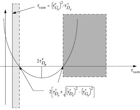
Fig. 4. Variation of quadratic which determines stability withτsum. That is to say, the reciprocal pole sum must be large enough. However, when (A) is fulfilled, the second term in (15) is neg-ative. Rewriting the left-hand side of it gives
LHS =τsum2 −4τDveτsum+ 4
τGve2. (18)
The function designated LHS is called the stability function, and is a quadratic inτsum. By considering the first and second derivatives, this parabola can be shown to have a minimum at 2τDve. The zero-crossing points are given by
τsum = 2
τDve±τv De
2
−τv Ge
2
. (19)
Obviously, both of these points are on the right-hand side of the vertical axis, hence the shape of the parabola (Fig. 4). Now, if the sign under the radical in (19) is negative, its roots are complex, or in other words LHS will never become negative and (15) is always true. Hence, for potential instability to occur, the following must always be true
τDve2>τGve2. (20)
As proven in Appendix II, the line corresponding to the equality of (A) should appear to the left of the first zero-crossing as shown. Then for stability, τsum has to appear in the lightly hatched area, or to the right of the second zero-crossing point. Ifτsumis too small, the sign under the radical is positive, but a negative time constant results. If τsum is situated between the zero-crossing points, complex poles are derived. Finally, if τsum is to the right of the second zero-crossing point, rep-resented by the darkly hatched area, again, a stable solution results. Hence, from the zero-crossing points, the next condition is derived
τsum<2
τDve−τv De
2
−τv Ge
2
or
τsum >2
τDve+
τv De
2
−τv Ge
2
Now, the stability conditions have been identified, the values for τsum that give the best response for different switching events can be derived. Firstly, for the case of the victim driver switching, since all aggressors are grounded, the metric that gives the best solution is the sum of the open circuit time constants with reference to the victim driver, which is calledτp∗. This is simply the summation of the products of all capacitors connected to the victim line with the driving point resistance to each of those capacitors
τp∗=− k∈v
RvkkCSkv+Rvkk+Ra1
jj
CCva1
k
+Rvkk+Ra2
jj
CCva2
k +· · ·
. (21)
This is a good approximation for the sum of the pole time constants [32], giving
τ1v+τ2v =τp∗. (22)
Substituting (22) forτsum in (10) and (13) results in the zero time constant and pole time constants respectively, for the victim switching. Now, an inspection of (5) and (21) shows that
τp∗> τv
De. Since (20) has to be true for instability to occur, this
means that
τp∗>
τv Ge
2
τv De
. (23)
Therefore, (A) is always true, and the only possible stability violation in this case is (B); i.e., very occasionally, usingτp∗can result in complex poles. The physical interpretation of such an occurrence is that the sum of the open circuit time constants underestimates the reciprocal pole sum, which has been unusu-ally escalated by an aggressor or aggressors with exception-ally high parasitics. Because both exponential waveforms are either additive or subtractive unlike when an aggressor switches (where one is additive and the other is subtractive), the higher frequency pole does not have a significant impact. In fact, this form of instability is usually an indication of a very-low-frequency pole, which makes the prediction of the waveform straightforward. The simplest remedy therefore is to consider a single pole response, with the pole time constant being given byτv
De. This results in good accuracy as shall be shown
in the Section IV.
Secondly, to solve for the poles and zeros associated with an aggressor switching, (3), (7), (8), and (9) are combined to give
τai
De =τ
ai
z (24)
τai
Ge 2
=τai
z (τ ai
1 +τ ai
2 ). (25)
Now, the zero time constant is available immediately from (24), and dividing (25) by (24) results in the reciprocal pole sum
τai
Ge 2
τai
De
=τai
1 +τ2ai. (26)
The pole time constants can be obtained by substituting (26) as
τsumin (13). It can be seen from an inspection of the relevant expressions that potentially either of (A) or (B) can be violated. The solution without generating extra information about the circuit is to accept the next best approximation. That is to say, ifτsum is so small that it violates inequality (A), the simplest and most logical remedy is to increaseτsumso that it is in the lightly hatched area. When inequality (B) is violated, if τsum is less than the minima, it should be decreased so that it falls into the lightly hatched region; if it is greater than the minima, it should be increased so that it falls into the darkly hatched region. Since the equality will generate coincident poles that are not acceptable, the exact value should be chosen so that it is slightly greater than or less than the equality, which can be achieved with a percentage factor. From empirical evidence over a range of testbeds, it was seen that 1% provides the best accuracy. This is the only constant that cannot be predicted by the theory, and is unfortunately unavoidable, as any approach to preserve stability without resorting to higher order moments has to be approximate in nature.
Using this approach, the values thatτsumshould take in the different cases are summarized in Table I. Of the two, (A) being violated is by far the more common form of instability. This occurs when the dominant poles for the victim and the particular aggressor are very far apart on the frequency axis. Physically, this translates to a situation where the receiver node is charged extremely rapidly by a very strong aggressor (i.e., through a relatively very small time constant), and decays with a very long tail, dictated by the much larger time constant of the victim. Such behavior is common for far end coupling. The instability in the solution predicted by (13) occurs because the pole sum given by (26) accurately reflects the high-frequency nature of the poles in the aggressor’s charging path, butτv
Deand
(τv Ge)
2reflect the much lower frequency content of the victim’s
dominant poles, and the gap is too much to bridge. The remedy proposed to this situation is to increase the reciprocal pole sum just beyond the threshold of the equality. Now, this yields accurate results, because the intention is to generate the best two-pole–one-zero model; in other words, the poles and zeros need not equate to the actual poles and zeros of the system, and indeed should differ for a second-order approximation. Using the factor of 1% beyond the threshold, which yields coincident poles, ensures that both the high- and low-frequency behavior is matched. It must be emphasized that conditions (A) and (B) are violated infrequently, and when they do, the values proposed above result in a simple yet accurate solution, which requires no extra information. The expressions for the reciprocal pole sum in body rows three to five of Table I represent the best approximations that guarantee stability when the first-choice approximations in rows one and two prove to be incompatible with the quadratic (13).
C. Physical Basis of the Model
TABLE I
VALUESTHATτsumSHOULDTAKE
properties—namely the area and first moment—of the actual waveform (step response) with the estimated waveform. The boundary conditions are already considered in the particular formulation of the transfer function (i.e., that the waveform starts and ends on a specific rail). Hence, matching the first and second moment of the impulse response does not define a unique solution, as a two-pole–one-zero transfer function has three unknowns. The necessary third equation is obtained by matching circuit components to the reciprocal pole sum.
For the switching of the victim driver with the other inputs grounded, the sum of the open circuit time constants provides a good approximation to the reciprocal pole sum, and combin-ing it with the moments of the circuit for the victim driver switching has a straightforward intuitive motivation. For the switching of an aggressor driver, the geometric properties of the actual waveform (via the first and second moments of the impulse response for an aggressor driver switching) are used to obtain the precise reciprocal pole sum. Since the quadratic (13) obtained from the moments of the impulse response for the victim driver switching contains relevant information about the victim net, combining it with the reciprocal pole sum for an aggressor switching gives a good approximation to the best two-pole–one-zero model. This is a procedure that works for the vast majority of circuits; however, some adjustments are necessary to the reciprocal pole sum for certain pathological cases, which was analyzed in a systematic manner, resulting in Table I.
D. Computational Complexity
1) Background—Incremental Computation of the Elmore Delay: The Elmore delay, as mentioned before, has been and is used extensively as a delay metric in VLSI interconnection circuits modeled by a tree where all capacitors are grounded, which is termed a simple tree. Simple trees are characterized by nodes that may have multiple children but only one parent. The Elmore delay is defined as
τDe =
k∈tree
RkeCk.
Consider the simple tree given in Fig. 2, where the output node is designated ase. According to the definition, the Elmore delay is
τDe=R1C1+ (R1+R2)C2+ (R1+R2+R3)C3
+ (R1+R2)C4+ (R1+R2)C5. (27)
This can be rearranged so that the expression is in terms of the product of the downstream capacitance and resistance at each node on the path from the source to the sink
τDe=R1(C1+C2+C3+C4+C5)
All downstream capacitances can be stored at each node by traversing the tree once. Hence, after one traversal of the complete tree, the computation of the Elmore delay at any node requires only that the path from source to sink for that particular instance be traversed, with the product of the resis-tance and downstream capaciresis-tance at each node being summed up. Because of this property, any changes to the capacitance values at any node in the tree require only that those changes be propagated upstream of those nodes where the changes took place. This is known as incremental computation, as only those cached values that are stale need to be updated. Any change to a resistance need only be considered when the metric with respect to a particular node is required, and the path from the root to that node is traversed. Incremental computation bestows considerable savings, and it is one of the principal reasons for the popularity of the Elmore delay.
2) Computational Complexity of Proposed Metrics: Alto-gether, five metrics that depend on the circuit topology are required for the proposed models. The first-order metrics are (5), (7), and (21), and the second-order metrics are (6) and (8).
First-order metrics: An inspection of the first-order met-rics (5) and (7) clearly shows their similarity to the Elmore delay. These can be rearranged so that the expressions are formulated as the sum of the products of resistance and down-stream capacitance at each node on the path from source to sink. Because of the extra complexity introduced by the coupling capacitances, it is necessary to keep track of individual coupling capacitances at each node. This can be achieved by caching the sum of the downstream self (or total) capacitances, and the sum of the individual downstream coupling capacitances with associated root information at each node. Hence, similar to the Elmore delay, all downstream capacitances are cached from a full tree traversal, and then the output with respect to a particular nodeeonly requires a traversal from the source toe. Also similar to the Elmore delay, any changes to the tree require only that the capacitance changes be propagated to the upstream nodes, resulting in incremental computation being possible.
The final first-order metric (21), the sum of the open circuit time constants, requires that at each node in the summation, that node should be treated as the output. Since the output node is therefore always defined for a given victim net (unlike in the previous metrics where the output can be any node in the tree), the incremental components of the summation in τp∗ can be cached along with the downstream capacitance. For example, in Fig. 1, node 4 should haveCS5as downstream self capacitance, andR5·CS5 as downstreamτp∗ information. Therefore, this metric requires no extra traversals at all, but instead, it can be computed along with the downstream capacitances. Again, changes to the tree require only that the changes be propagated to upstream nodes.
Second-order metrics: The second-order metrics require the capacitances at each node be weighted individually by a first-order time constant, which is basically expression (4) (in one of the three forms used) for the path defined from the root of the relevant simple tree to the current node, or its coupled counterpart. There are now three issues related to complexity:
1) How much work is needed to calculate the weights for the original tree?
2) When the weights are known, how much work needs to be done to calculate the second-order metrics with respect to a particular node?
3) Finally, how much work needs to be done to recalculate all the weights once a change or changes have been made to the tree?
Calculation of the weights is demonstrated on the victim net of Fig. 1. The weights required are different for the two ex-pressions, and also for the types of capacitances (i.e., coupling capacitance between two trees, or the total capacitance, at a particular node), but are always characterized in a generic sense by the expression (4). Hence, any technique that works for one will always work for all the weights. For the sake of explanation, assume that the weight consists ofτv
Dk, where only
self capacitances are considered, and that the weights at nodes 1 and 2 areτ1andτ2, etc. Then
τ1=R1(CS1+CS2+CS3+CS4+CS5) (29)
and
τ2=R1(CS1+CS2+CS3+CS4+CS5)
+R2(CS2+CS3+CS4+CS5). (30)
The rest of the metrics are calculated in a similar manner. Now, since the weight is always with respect to the root, it is necessary to visit all the nodes once after the downstream capacitance information has been stored on the initial pass. (It is useful also to store the upstream resistance at each node on this pass, so that in future visits to the node, theτinformation can be updated instantly, as will be shown later.) All weights can be calculated in one pass by using the property that
τDvn =τDvm+τDvm→n (31)
where nodemis situated on the path between the root and node
n. At branch points, a depth first traversal of all child branches preserves the linearity of the traversal. Hence, the weights for all nodes can be calculated by one full tree traversal once the downstream capacitance information has been stored.
The answer to the second question is straightforward; an inspection of (6) and (8) shows that the form that the outer (second order) summation takes is exactly similar to the inner (first order) summation, which is characterized in a generic way by the expression (4). Therefore, it is possible to cache the downstream τ·C information (just as the downstreamC
information was cached for the first-order metrics) and obtain the metrics from the root to a particular node by visiting only the nodes along the path from the root to that node.
So far, two complete traversals have been necessary, one bottom-up pass to store the downstream capacitance informa-tion, and one top-down pass, beginning at the root to store the
path from the root to that node. Again, if an imaginary second-order metric is defined to consist only of the self capacitances for simplicity of explanation, the value that would be cached at node 5 on the third (bottom-up) traversal would beT5=T5·
CS5, that at node 4 would beT4=T5+τ4·CS4, and so on. Hence, three full traversals are necessary, one bottom-up traversal to store the downstream capacitance information, one top-down traversal to store the weights, and a final bottom-up traversal to store the downstreamτ·C information. None of these passes can be combined as the necessary order is bottom-up, top-down, and bottom-up.
The only remaining question is also the most important; if it is necessary to traverse the entire tree three times each time a change is made, the incremental computation property is lost. However, after a modification to a component, since only the resulting changes in the stored values need to be accounted for, the calculations that required three traversals for the original tree can be accomplished in one traversal. Consider, for example, that the component valueCS2is changed toCS2. This immediately causes:
1) the downstream capacitance values cached at node 2 and all nodes upstream of node 2 to be stale;
2) the cached weight(τ)information at all nodes to be stale; 3) the cached downstreamτ·Cinformation at all nodes to
be stale.
In node 5, for example, the stored downstream capacitance is current (since the changed capacitor is upstream of it), but the weight and downstreamτ·Cinformation is stale. The old weight is
τ5=R1(CS1+CS2+CS3+CS4+CS5)
+R2(CS2+CS3+CS4+CS5)
+R4(CS4+CS5) +R5(CS5). (32)
The new weight is
τ5 =R1(CS1+CS2 +CS3+CS4+CS5)
+R2(CS2 +CS3+CS4+CS5)
+R4(CS4+CS5) +R5(CS5). (33)
The change is
τ5−τ5= (R1+R2) (CS2 −CS2). (34) Therefore
τ5 =τ5+ (R1+R2) (CS2 −CS2). (35) This is simply the change in the capacitance multiplied by the resistance that is upstream of the changed capacitance. This is true of all nodes downstream of node 2. At the nodes upstream of node 2, the capacitance change is multiplied by the upstream resistance from that node. Similarly, the downstream
τ·Cinformation can also be calculated and stored. Hence, all stale information can be updated by doing a single bottom-up traversal by considering the difference introduced by the change to the component. First, the changed component is
located, and its upstream resistance (R1+R2), which has been stored earlier, is noted. Now, starting from a leaf node, say node 5, for example, a bottom-up traversal is initiated, where both the weight information and the downstreamτ·C
information are updated at once. From node 2 upwards, the downstream capacitance also needs to be updated. Hence, the original requirement of three passes for the unprocessed tree has been reduced to a single pass. This principal also applies for resistor changes, and also multiple component changes. That is, the effect of multiple changes can be considered in one pass.
Summary: It was shown that all the metrics have a very simple and small core, which exactly resembles the Elmore de-lay. The second-order expressions can be described as a weight-ed Elmore delay; each term in the summation is weightweight-ed by either (5) or (7) for that particular node. These are similar to the second moment of the impulse response proposed for sim-ple trees in [4]. Just as the models of [4] represent the minimum computational complexity for second-order models for the class of circuits that were called simple trees, these models represent the minimum complexity for coupled trees. In fact, if the cou-pling capacitance terms are put to zero (the entire capacitance is lumped into a ground component), the model for the victim tree reverts to the model proposed in [4].
One of the major attractions of the Elmore delay is its in-cremental computational property. This is a very useful feature, and is the mainstay of several interconnect optimization algo-rithms. It should be noted that this is independent of the output node. Whatever node is chosen asein the tree, this hierarchical property holds true. Now, since the constituent summations in the proposed metrics have exactly the same form as the Elmore delay, whose format is basically that of (4), incremental com-putation is possible for the proposed metrics.
3) Comparison With Other Metrics: As shown in Section II, there are an enormous number of models both of a general nature that are not restricted to second-order estimations, and ones that are explicitly second-order. In this section, it is shown that the proposed model has the least complexity of all two-pole–one-zero models in both categories. It is useful to start the discussion with a look at the general techniques AWE [13] and RICE [14].
computation of the higher order moments that require four extra traversals is avoided. For component value changes, the general property of incremental computation would hold, but it would necessarily be more expensive for four moments. The first moment (Elmore delay) requires component values to be propagated upstream only; the second moment requires one full tree traversal as has been shown; similarly, the third and fourth moments would require two and three traversals. Therefore, the proposed model saves two full tree traversals for component value modifications.
As mentioned earlier, the model that best merits comparison with the proposed model is [19], the other second-order models either being restricted in topology (such as [4]—simple trees; [17], [18], and [22]—inductive trees with no series capacitors; [26], [27]—parallel lines), restricted in accuracy (such as [20] and [31], which use the same poles for all responses), or lacking a clear physical basis (such as [23] and [24]), which do not translate to a two-pole–one-zero model, and hence cannot be used to generated the responses for aggressors switching, and are less accurate than direct moment matching for the vic-tim switching. When the moments are computed with the algo-rithms of [14], the explicit two-pole–one-zero model of [19] is the least expensive second-order model that can handle arbi-trarily coupledRCtrees reported in the literature. Because the proposed model does not require the third moment of the impulse response, it is cheaper than this model by the equivalent of at least two full tree traversals for the unprocessed tree, and at least one full tree traversal for component value changes. Be-cause incremental physical optimization requires many changes to the interconnection tree, the proposed model will often save two complete tree traversals, a huge saving for any reasonably sized circuit. The comparison carried out in Section IV shows that this saving is not at the expense of loss in accuracy.
Finally, it is worth looking at the complexity of circuit collapsing techniques such as passive PRIMA [16], as they only require q moments to generate a qth-order response. In PRIMA, the most critical steps in terms of runtime are an LU decomposition and qN backward and forward substitu-tions for an N-port circuit, which corresponds to a qth-order response, both of which must be performed on the modified nodal analysis (MNA) matrix of the original network. The LU factorization already makes the complexity at least as much as the three complete traversals required for the un-processed tree in the proposed methodology. The most ef-ficient manner in which the second can be accomplished is by recursively solving an equivalent DC circuit as in [13]. Hence, the computation of each block moment requires at the minimum one backward and forward substitution, which is equivalent to two tree traversals. Furthermore, there is an overhead introduced by the orthogonalization and orthonormal-ization procedures, which makes the complexity of a block moment computation more than the equivalent of two tree traversals. This is neglecting the overhead of setting up the MNA matrix, which has to follow the setting up of the spanning tree (unless the netlist is already appropriately ordered, which is not the general case). Hence, the complexity of a second-order Krylov space projection-based approximation does not really bear comparison to the proposed methodology. Such
network collapsing methods are suitable for macromodeling linear blocks by higher order approximations, not for incremen-tal physical optimization.
E. Peak Noise and Delay to Peak Noise
In this paper, the generation of the transfer function, which is the most important aspect of the modeling, is the main concern. Choice of input waveform, driver modeling, and subsequent processing of the waveform depend on the application, and are not covered for the most part. Knowing the transfer function allows the output to be generated for the appropriate input by a number of approaches, including table look-up and heuristic expressions. Explicit expressions are, however, derived for step inputs, which are sufficiently accurate for quite a number of applications. First, the step response at nodeewhen the victim driver switches is given by
Eev(t) = 1−τ v 1 −τzv
τv 1 −τ2v
e−
t τ v1 −τ
v z −τ2v
τv 1 −τ2v
e−
t τ v2
. (36)
The step response when an aggressor driver switches is
Eai
e (t) =
τai
z
τai
1 −τ ai
2
e−
t τai
1 −e − t
τai
2
. (37)
It is not possible to solve a two-pole (or higher order) wave-form explicitly for the delay at a given threshold. Closed-wave-form heuristics for a two-pole waveform can be derived—such as in [19]—but since the complete response for anmdriver system will consist of2mexponential waveforms, some iterative pro-cedure needs to be adopted in the general case.
However, (37) can be solved explicitly for the peak noise, and the time at which it occurs. Equating the first time derivative to zero and doing some trivial algebra results in
tpk=
τai
1 τ ai
2 (τai
1 −τ2ai) lnτ
ai
1
τai
2
. (38)
Substituting (38) fortin (37) results in the peak noise from the switching of the driver of aggressor ai. Knowing the times at which the individual peaks occur is extremely useful in algo-rithms to process the waveform for delays at a given threshold, when multiple drivers switch at different times. A temporal window can be defined, which is bounded by the first peak and last peak; these peak values can be used as initial guesses for fast and true convergence with the Newton–Raphson algorithm, even for multiple-time constant waveforms.
IV. RESULTS
TABLE II
AVERAGEPERCENTAGEERRORS INDELAYS ATDIFFERENT
THRESHOLDS FORVICTIMSWITCHING
distribution models from three moments described in [33] and [24], and the gamma probability distribution model from two moments, also described in [33]. It should be noted that the probability distribution models are valid only for the victim switching. Here, the model is extensively tested against the Elmore delay, the closest less expensive model, and the two-pole–one-zero model from three moments, the closest more expensive model, in thousands of comparisons with the re-sponse from a Spice3 simulation serving as the yardstick of the actual waveform. Since the actual and predicted delay at a single threshold can agree very well, and still result in significant deviations along the full waveform, the accuracy was tested at three points along the waveform. For the victim switching, the thresholds are 10%, 50%, and 90%, while for the aggressors they are 25%, 100%, and 25% of the peak amplitude. This is to ensure that three points, with two being on either side of the peak, are tested. The average results are shown in Tables II and III. The numbers shown in each case is the error calculated as a percentage against the actual value as given by Spice; a negative number means that the predicted value was greater than the actual and vice versa. Hence, the smaller the magnitude of the number, the better; a value of zero means zero error. These numbers do not have much significance as indicators of absolute error, but are very useful for comparisons between models.
Different kinds of circuits were grouped into the four cluster categories. The test nodes comprise all nodes in each circuit in each case, covering all possible circumstances such as near-end and far-near-end coupling and stiff nodes. It can be seen that the proposed model performs very well against the more expensive model computed from three moments, and is in fact often better in the delay predictions. The only area in which it is consistently outperformed by the three moment model is in peak noise
TABLE III
AVERAGEPERCENTAGEERRORS INDELAYS ATDIFFERENTTHRESHOLDS ANDAVERAGEERROR INPEAKNOISE FORAGGRESSORSWITCHING
prediction, to varying degrees. However, as the point of the proposed model is to use as a metric of comparison between different topologies, this need not be any kind of limitation in its intended applications of incremental physical optimization and global signal planning.
V. SUMMARY ANDCONCLUSION
Closed-form expressions for the first two moments of the impulse response for general arbitrarily coupledRCtrees with multiple drivers were presented and used to generate stable and accurate second-order approximations to the transfer function for any switching event. For the victim driver switching, the sum of the open-circuit time constants with regard to the victim net is used to avoid using higher order moments. For the case of an aggressor driver switching, the moments for the victim and aggressor switching are combined, which can be described as an averaging of the dominant poles along the victim and that aggressor. This procedure provides the best opportunity to match the waveform along the charging and discharging paths while saving on higher order moments. The summation of all waveforms result in the complete response at the node of interest. This model represents the minimum complexity for a general second-order model for this class of circuits, and is hence proposed as being useful for initial estimates of delay and noise in complex systems early in the design flow, and particularly for incremental physical optimization.
APPENDIXI
COMPUTATION OFMOMENTS
When the victim driver switches while all other inputs are grounded, the first moment of the impulse response at the output nodeeis given by
Υ1e=
∞
0
thve(t)dt. (39)
Now, the following expression describes the voltage drop from the source to e where Ev
e(t) is the step response at e, and a1, a2, . . . are the aggressors. This is obtained by sum-ming up the capacitor currents and adding the drops across each resistor, or in other words, using Kirchoff’s voltage and current laws
1−Eev(t) =
k∈v
Rvke
CSkv dEv
k dt +CC
va1
k
dEva1
k dt
+CCva2
k
dEva2
k
dt +· · ·
. (40)
The impulse responsehv
e(t)is the first time derivative of the step response. Hence, (39) can be integrated by parts, and (40) substituted in it to yield the following expression
Υ1e= k∈v
Rvke[CSkv+CCva1
k +CC
va2
k +· · ·] =τ v De say.
(41)
The second moment of the impulse response at the output nodeeis given by
Υ2e=
∞
0
t2hve(t)dt.
Integrating by parts, it can be shown that this is equivalent to
Υ2e= 2
∞
0
t(1−Eev(t)) dt.
Using the above expression for the step response and again integrating by parts, this can be shown to be
Υ2e= 2 k∈v
Rvke
CSkv
1
0
tdEkv+CCva1
k 1
0
tdEva1
k
+CCva2
k 1
0
tdEva2
k +· · ·
. (42)
The constituent integrals can be evaluated by integrating by parts and using Kirchoff’s laws to obtain expressions for the voltages. The first integral is basically the first moment at
node k, for which an expression can be obtained by simply substitutingkforein (41). The other integrals are of the form
Iai=
1
0
tdEvai
k .
Integrating by parts, this simplifies to
Iai =
∞
0
[1−Evai
k (t)] dt.
The voltage can be decomposed into two components thus
Evai
k =E
v
k−E
ai
j .
Now, circuit laws can be used to obtain expressions for the individual voltages. This first is
1−Ekv(t) = K∈v
RvKk
CSKv dE
v K dt +CC
va1
K dEva1
K dt
+CCva2
K dEva2
K dt +· · ·
and the second
Eai
j =
K∈ai
Rai
Kj
CSai
K dEai
K dt +CC
aiv
K dEaiv
K dt
+CCaib1
K
dEaib1
K
dt +CC
aib2
K
dEaib2
K
dt +· · ·
.
The superscriptsaib1, aib2. . .in theCC terms indicate the coupling capacitances to treeai’s own aggressors. Considering the fact that all nodes not on the victim tree start and end at the same voltage, this simplifies to
Υ2e= 2 k∈v
Rvke
×
CSvk
K∈vic
RvKk(CSKv +CCva1
K +CC
va2
K +· · ·)
+CCva1
k
K∈a1
Ra1
KjCC
a1v
K +
K∈v
RvKk
×(CSKv +CCva1
K +CC
va2
K +· · ·)
+CCva2
k
K∈a2
Ra2
KjCC
a2v
K +
K∈v
RvKk
×(CSKv +CCKva1
+CCva2
K +· · ·)
+· · ·
This can be expressed in more succinct form by using the first moment of the impulse response
Υ2e
= 2
k∈v
Rvke
CSkvτDvk+CCva1
k
τDvk+ K∈a1
Ra1
KjCC
a1v
K
+CCva2
k
τDvk+
K∈a2
Ra2
KjCC
a2v
K
+· · ·
= 2τGve2 say.
Following an approach identical to that in the former case, the first moment of the impulse response at nodeeon the victim tree for aggressoraiswitching can be shown to be
Υ1e=− k∈v
RvkeCCvai
k =−τ
ai
Desay.
The second moment can also be calculated from an approach similar to the former case, resulting in
Υ2e
=−2 k∈v
Rvke
×
(CSkv+CCkva1+CC va2
k +· · ·)τ ai
Dk+CC
vai
k
×
K∈ai
Rai
Kj
CSai
K +CC
aiv
K +CC
aib1
K +· · ·
=−2τai
Ge 2
say.
APPENDIXII
BEHAVIOR OFSTABILITYFUNCTION
In this section, it is proven that the equality of (A) is always to the left of the first zero-crossing point of LHS, which is important in analyzing the physical basis of potential instability. Since the following is true [where the last condition is necessary for potential instability to occur—see the explanation for (20) in the main text]
τDve>0 τGve2>0 τDve2>τGve2
the following holds true
4τDve2−τGve2 +
τv Ge 4 τv De
2 >4
τDve2−τGve2
i.e.,
2τDve 2 − τv Ge 2 τv De 2 >
2τv De
2
−τv Ge
22
when
2τDve−
τv Ge 2 τv De
>2τv De
2
−τv Ge
2
.
Rearranging the terms results in
τGve2 τv
De
<2
τDve−τv De 2− τv Ge 2 .
Hence, the equality of (A) is always to the left of the first zero-crossing point of LHS.
ACKNOWLEDGMENT
Very productive discussions with Dr. L.-R. Zheng of the Laboratory of Electronics and Computer Systems, Department of Microelectronics and Information Technology, Royal Insti-tute of Technology, Sweden, are gratefully acknowledged.
REFERENCES
[1] SEMATECH. (2003). International Technology Roadmap for Semicon-ductors (ITRS). [Online]. Available: http://public.itrs.net/Files/2003ITRS/ Home2003.htm
[2] D. Pamunuwa, S. Elassaad, and H. Tenhunen, “Modelling noise and delay in VLSI circuits,”Electron. Lett., vol. 39, no. 3, pp. 269–271, Feb. 2003. [3] ——, “Analytic modeling of interconnects for deep sub-micron circuits,”
in Proc. Int. Conf. Computer-Aided Design (ICCAD), San Jose, CA, Nov. 2003, pp. 835–842.
[4] M. A. Horowitz, “Timing models for MOS circuits,” Ph.D. dissertation, Stanford Electr. Lab., Stanford Univ., Stanford, CA, Jan. 1984.
[5] E. Chiprout, “Interconnect and substrate modelling and analysis: An over-view,” IEEE J. Solid-State Circuits, vol. 33, no. 9, pp. 1445–1452, Sep. 1998.
[6] D. Pamunuwa, L. R. Zheng, and H. Tenhunen, “Maximizing throughput over parallel wire structures in the deep submicrometer regime,”IEEE Trans. Very Large Scale Integr. (VLSI) Syst., vol. 11, no. 2, pp. 224–243, Apr. 2003.
[7] A. Deutschet al., “When are transmission lines important for on-chip interconnects,” IEEE Trans. Microw. Theory Tech., vol. 45, no. 10, pp. 1836–1846, Oct. 1997.
[8] I. Ismail, E. G. Friedman, and J. L. Neves, “Figures of merit to character-ize the importance of on-chip inductance,”IEEE Trans. Very Large Scale Integr. (VLSI) Syst., vol. 7, no. 4, pp. 442–449, Dec. 1999.
[9] K. Banerjee and A. Mehrotra, “Analysis of on-chip inductance effects using a novel performance optimization methodology for distributed RLC interconnects,” inProc. Design Automation Conf. (DAC), Las Vegas, NV, 2001, pp. 798–803.
[10] W. C. Elmore, “The transient response of linear damped circuits,”J. Appl. Phys., vol. 19, no. 1, pp. 55–63, Jan. 1948.
[11] J. Rubinstein, P. Penfield, and M. Horowitz, “Signal delay in RC tree networks,” IEEE Trans. Comput.-Aided Des. Integr. Circuits Syst., vol. CAD-2, no. 3, pp. 202–211, Jul. 1983.
[12] C. Y. Chu and M. A. Horowitz, “Charge-sharing models for switch level simulation,”IEEE Trans. Comput.-Aided Des. Integr. Circuits Syst., vol. CAD-6, no. 6, pp. 1053–1061, Nov. 1987.
[13] L. T. Pillage and R. A. Rohrer, “Asymptotic waveform evaluation for timing analysis,”IEEE Trans. Comput.-Aided Des. Integr. Circuits Syst., vol. 9, no. 4, pp. 352–366, Apr. 1990.
[14] C. L. Ratzlaff, N. Gopal, and L. T. Pillage, “RICE: Rapid intercon-nect circuit evaluator,” inProc. Design Automation Conf. (DAC), San Francisco, CA, 1991, pp. 555–560.