Comparative Analysis of Machine Learning Algorithms for their Effectiveness in Churn Prediction in the Telecom Industry

© 2017, IRJET | Impact Factor value: 5.181 | ISO 9001:2008 Certified Journal

| Page 485

Comparative Analysis of Machine Learning Algorithms for their

Effectiveness in Churn Prediction in the Telecom Industry

Mr. Nand Kumar

_{, Mr. Chetankumar Naik}

---***---Abstract - Churn is a term that gives insights of the attrition rate of the customer in any particular company. Telecom industry is highly dynamic in industry in nature; highly active in terms of customer relationship and management compared to any other industry but the customer base is tend to be fragile because of the luring offers offered by competitive companies to get strong hold the customer base which results into customer churn, thereby affecting the company’s customer’s assessments due to the liquidity. This paper aims at providing solution to this problem by identifying the potential customers who tend to switch to other companies by using different machine learning algorithms and evaluation each for their effectiveness. Data analysis is done on previously recorded data for extracting the potential features and their dependencies that impact on the churn. State of art classification algorithms like balanced logistic regression, random forest and balanced random forest are used. To optimize the solution, thorough analysis of the performance is done and based on the measure of goodness of the algorithm; the one that fits best is identified. The output obtained will help the company to control the attrition rate by handling their issues on time and retaining them with the company.

Key Words: — Balanced Logistic Regression, Churn,

Classification, Data pre-processing, key feature extraction, Principal Component Analysis, Random forest

1. INTRODUCTION

The churn rate, also known as the rate of attrition, is the percentage of subscribers to a service who discontinue their subscriptions to that service within a given time period. For a company to expand its clientele, its growth rate, as measured by the number of new customers, must exceed its churn rate[1].

There are an ample number of reasons for a company to lose its customers. The primary reason is the cost of the product, the product quality and quality of service. The valuation of any company is affected if the customer

outflow is very high. Many companies lose its

reputation amongst its stakeholders.

However, for the customer to be retained, it is very important to also measure customer satisfaction. Evaluating the degree of customer satisfaction is a difficult task. It becomes more difficult when the customer base accounts up to millions. Value added service is another

reason for Churn. Telecom companies have started a newoffering called Triple play [2], combining the TV, broadband and the phone offering as compared to the traditional model of just the phone services. This is seen as a value adds to retain customers. The Triple play not only helps retain customers but also increases the Average revenue per user (ARPU) directly contributing to the revenue of the company [3].

1.1 How to Reduce Churning:

1 “After sales service” is of prime importance.

Person consideration is very important when it comes to the service part so that the customer feels privileged.

2 Customized offers should be provided based on

their expenditure.

3 Value added services should be enhanced

4 Trust building by handling each individual’s query

and

resoling queries on time will manifest returns.

2. LITERATURE SURVEY

Telecom companies have used two approaches to address churn –

a) Untargeted approach: Mass-marketing and creating

brand loyalty for the product

b) Targeted approach: Involves focusing on the

customer base likely to churn. Intervening with the personal care and taking steps to avoid their likeability to churn

Targeted approach needs to derive some important insights which is difficult to be evaluated manually since the data is very dynamic and large. The machine learning techniques have evolved to a great extent assisting intelligent solutions to churn issues that are present in the telecom industry. The researchers have come up with significant algorithms that are proven to give valuable insights over the given data. The problem that is being taken up is of the classification of customers on evaluation of their potential to churn based on several factors.

© 2017, IRJET | Impact Factor value: 5.181 | ISO 9001:2008 Certified Journal

| Page 486

1 Number of observations: 25000

2

3

No of variables: 111(Independent=110 target=1)

Number of missing values: No missing values and algorithms used in machine learning for this particular problem which can further provide solution for the problem with similar inputs. The thorough analysis of the algorithms will give a clear picture about the accuracy of each. The final result of the analysis will decide on the best solution with minimal errors.

3. METHODOLOGY

1 Understanding t h e b u s i n e s s p r o b l e m i s h i g h l y important, evaluating which a final structure of the problem can be devised with confidence. 2 The next step inculcates understanding the data and its

interdependency; correlation among different

variables should be done.

3 PCA for Feature Selection, new dimensions, pre- processing

4 Build Logistic regression Model for Classification 5 Balance data using smote + Logistic Regression 6 Classification using Random Forest (35 PCA) 7 Classification using Random Forest (4 important PCA)

8 Random forest in H2O – Parameter Tuning 9 The final outcome is analyzed

The accuracy of the test depends on how well the test separates the group being tested into those with and without the disease in question. Accuracy is measured by the area under the ROC curve. An area of 1 represents a perfect test; an area of .5 represents a worthless test[7].

3.1 Data Exploration

Complex structure of data implies new, sophisticated

solutions including data transformation, semantic

representation and new mathematical theories

accommodation. The most important problem of

data processing is to make sense of available data[4].

The data is provided by the telecom company which needs some preprocessing. Given below are the details about the data

3.2 Principal component analysis for Feature Selection

Principal component analysis is a method of extracting important variables (in form of components) from a large set of variables available in a data set. It extracts low dimensional set of features from a high dimensional

data set with a motive to capture as much information as possible. With fewer variables, visualization also becomes much more meaningful. PCA is more useful when dealing with 3 or higher dimensional data [5].

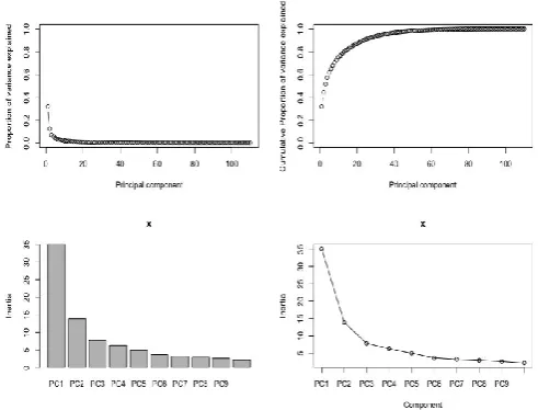
Since the data to be worked on is of very high dimension. It becomes necessary to eliminate the dimensions such that the model works effectively without much unnecessary and irrelevant computation, which can end up getting unwanted results. It is proven that the first principal component involves the dimensions that are highly important, followed by the second component and so on. It is the data expert who can understand the problem better can decide on the rightnumber of components to used in order to provide the right input to the model

Fig -1: Principal Components

3.3 Stratified Sampling

Stratified Sampling with train and validation in the ratio 7:3 set.seed(1000)

split = sample.split(data_Pca_less_Comp$target, SplitRatio = 0.70)

# Split up the data using subset

train = subset(data_Pca_less_Comp, split==TRUE) test = subset(data_Pca_less_Comp, split==FALSE)

3.4 Build Logistic regression Model for Classification

© 2017, IRJET | Impact Factor value: 5.181 | ISO 9001:2008 Certified Journal

| Page 487

dependent binary variable and one or more nominal, ordinal, interval or ratio-level independent variables[8]

Logistic Regression using train data set and 35 Components from P.C.A The results below are obtained by running the model in RStudio. The glm() function is used to apply logistic regression on the given data.

LogReg <- glm(target~.,data = train,family = "binomial”) Inference:

Accuracy on Train Set: 0.79

Accuracy on Test Set: 0.80

Recall on the Test Set: 0.58

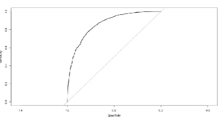
The graph below is obtained in the Rstudio

Fig -2: ROC for Logistic regression Model

The Area Under Curve is: 0.8547 for logistic regression model

3.5 Logistic Regression Using Smote

We witnessed a low recall. Data is not completely imbalanced, but building a model on a completely balanced data could help

Use SMOTE to balance the data

train_smote=SMOTE(target~.,data=train, perc.over=100,perc.under=200)

prop.table(table(train_smote$target))

Fig -3: ROC for Logistic regression Model using smote

Area Under Curve: 0.861

Accuracy on Train Set: 0.78

Accuracy on Test Set: 0.77

Recall on the Test Set: 0.76

3.6 Classification using Random Forest

Random forest (Breiman, 2001) is an ensemble of unpruned classification or regression trees, induced from bootstrap samples of the training data, using random feature selection in the tree induction process.

Prediction is made by aggregating (majority vote for classification or averaging for regression) the predictions of the ensemble. Random forest generally exhibits a substantial performance improvement over the single tree classifier such as CART and C4.5 [6]. It yields generalization error rate that compares favourably to Adaboost, yet is more robust to noise. However, similar to most classifiers, RF can also suffer from the curse of learning from an extremely imbalanced training data set.

The model was executed in Rstudio. The output below is its summary extract

Fig-4: Summary for the performance of random forest model for 35 principal components

© 2017, IRJET | Impact Factor value: 5.181 | ISO 9001:2008 Certified Journal

| Page 488

Fig -5: ROC for the random forest model with 35 principal components

Inference:

Area Under Curve: 0.8324 we chose mtry = 5, ntree=50)

The area under the ROC curve is 0.83, which is less when compared to that of the logistic regression model.

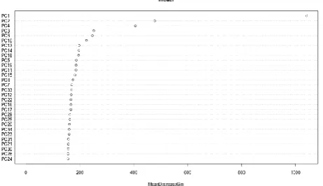
Fig -6: Random forest using top 4 importantAttributes

Fig-7: Summary for the performance of random forest model for 4 principal components

3.6 Random forest in H2O

1. We will use parameter tuning to find the values of mtry and ntree to give us the best AUC

2. Import the dataset into H20

3. Grid Search and Model Selection with H2O and define the tuning parameter -> mtries

Fig -8: H2O grid details

Inference:

Mtry=8 gives us the best model

The AUC is calculated on Out of Bag Samples. Hence cross validation is not needed.

4. CONCLUSION

The various model presented in the paper had good accuracy rate but the Logistic regression model on the balanced data has the highest area under the curve, which by convention proves to be the best model delivering high Accuracy and is more parsimonious model

REFERENCES

[1] ]http://www.investopedia.com/terms/c/churnrate.asp

[2]

https://en.wikipedia.org/wiki/Tripleplay_(telecomm uni cations)

[3]

http://www.happiestminds.com/whitepapers/how-to- reduce-churn-in-a-telco-industry [4]

http://www.academia.edu/4506159/Top_Challenges_of _Data_Processing

[5]

https://www.analyticsvidhya.com/blog/2016/03/pra

© 2017, IRJET | Impact Factor value: 5.181 | ISO 9001:2008 Certified Journal

| Page 489

[6] http://statistics.berkeley.edu/sites/default/files/tech- reports/666.pdf

[7] http://gim.unmc.edu/dxtests/roc3.htm