Modelling and simulation for the
joint optimisation of inspection
maintenance and spare parts
inventory in multi-line
production settings
Farhad Zahedi-Hosseini
PhD Thesis
Salford Business School
University of Salford
The studies developed in this PhD thesis form the basis for three journal papers, as detailed
below:
1. The material in Chapter 3 has been developed into a paper for the European Journal of
Industrial Engineering. The original manuscript was submitted on 6th October 2016. The revised manuscript was submitted on 29th April 2017; this is currently under review.
2. The study in Chapter 4 has been developed into Zahedi-Hosseini et al. (2017), which
was published online on 12th March 2017, and appeared in the Journal of Reliability Engineering and System Safety 168: 306-316.
3. Finally, the work in Chapter 5 is being prepared for a paper to be submitted to the
A simulation methodology is developed to model the joint optimisation of preventive maintenance
and spare parts inventory in multi-line settings. The multi-line machines are subject to failure, based
on the delay-time concept, and a selection of policies are used for the replenishment of the machines’
critical component. Production lines of varied configurations are modelled and described in three
principal chapters.
Firstly, the optimisation of preventive maintenance for a multi-line production system is
developed in the context of a case study. The policy proposed indicates that consecutive inspection
with priority for failure repair is cost-optimal, which suggests a substantial maintenance cost
reduction of 61% compared to the run-to-failure policy. The contribution of this study is first and
foremost in narrowing the gap between the theory and practice of managing multi-line systems, and
in particular, that the scenarios and policies considered have important economic and engineering
implications.
In a second study, spare parts provisioning for a single-line system is considered, given that the
demand for industrial plant spare parts should be driven, at least in part, by maintenance
requirements. A paper-making plant provides a real context, for which simulation models are
developed to jointly optimise the planned maintenance and the associated spare part inventory. This
challenge is addressed in the context of the failure of parts in service and the replacement of
defective parts at inspections of period 𝑇, using the delay-time concept, and a selection of
replenishment policies. The results indicate that a periodic review policy with replenishment twice
as frequent as inspection is cost-optimal. Further discussions and sensitivity analysis give insights
into the characteristics and features of the policies considered.
Finally, in the third study, the joint optimisation of preventive maintenance and the associated
spare parts inventory for a multi-line system is developed using an idealised context. It is found that
a review policy with inspection as frequent as replenishment using just-in-time (JIT) ordering is
cost-optimal, and also the lowest risk policy; it is associated with the lowest simultaneous machine
downtime and low stock-out cost-rates. This is a significant contribution to the literature.
An implication of the proposed methodology is that, where mathematical modelling is
intractable, or the use of certain assumptions make them less practical, simulation modelling is an
appropriate solution tool. Throughout this thesis, the long-run average cost per unit time or cost-rate
is used as the optimality criterion. In other contexts, one may wish to use availability or reliability
IN THE NAME OF GOD
This PhD thesis is dedicated to the following people:
To my dear parents,
for their complete support during my long study years in the UK,
especially, to my late beloved father,
whose wish was for me to complete my PhD - may God bless his soul;
To my beautiful wife, Houri,
for her love, kindness, understanding, patience, and hard work;
To my gorgeous daughter, Dr. Delaram Zahedi, MBChB,
Acknowledgements
I would like to thank the following people whose help, guidance, advice, and encouragement,
were pivotal in the completion of this part-time PhD:
To my main supervisor, Professor Philip Scarf - a true expert in maintenance and mathematical modelling, whose vision, help, encouragement and deep knowledge of the
maintenance subject was invaluable in enabling me to better understand, analyse, and
interpret challenging issues in maintenance. Phil’s email discussions, sometimes during
late evenings and weekends, were invaluable, helpful, supportive, and highly
appreciated.
To my original supervisor, the late Professor Wenbin Wang, who sadly passed away
last year. His enthusiasm, help, guidance, and encouragement was invaluable in the early
stages of my research work. May God bless his soul. To my second supervisor,
Professor Aris Syntetos, whose help and advice in later years of my PhD was very helpful.
To Professor David Howard, my colleague, mentor, and a true friend, who helped and
encouraged me in various ways to start and continue my PhD. His encouragements and
long discussions gave me the audacity to start my PhD despite my family commitments
and full-time work. I’m very thankful to him for the continuation of help and
encouragement all throughout my PhD.
To Professor Tim Ritchings, our previous Head of School, Professor Sunil Vadera,
our current Dean of School, and Dr Tony Jones for their support and authorising the
Table of Contents
Preface --- 2
Abstract --- 3
Dedications --- 4
Acknowledgements --- 5
List of Tables --- 10
List of Figures --- 11
List of Appendices --- 15
List of Abbreviations --- 18
1. Chapter 1 Introduction --- 19
1.1. Background and methodology --- 19
1.2. Aims & objectives --- 21
1.3. Structure of this thesis --- 23
2. Chapter 2 Literature review and Notation --- 25
2.1. Maintenance systems --- 25
2.1.1. Delay-time modelling --- 29
2.2. Inventory control systems --- 35
2.3. Discrete-event simulation --- 37
2.4. Gaps in literature --- 44
2.5. Notation --- 44
2.5.1. Notation associated with Chapter 3 --- 44
2.5.2. Notation associated with Chapter 4 --- 45
2.5.3. Notation associated with Chapter 5 --- 46
3. Chapter 3 Optimisation of inspection maintenance for multi-line production systems --- 48
3.3. Modelling methodology --- 51
3.3.1. Notation --- 51
3.3.2. The delay-time model development --- 51
3.3.3. Modelling multi-line production systems --- 53
3.4. Case study --- 56
3.4.1. Problem description --- 56
3.4.2. Numerical example --- 57
3.4.3. Simulation modelling --- 58
3.4.4. Base model (validation) --- 62
3.4.5. ‘Modified’ two-out-of-three parallel system --- 63
3.4.6. ‘Standard’ two-of-three parallel system --- 64
3.4.7. Three-parallel lines system --- 65
3.4.8. Sensitivity analysis --- 67
3.5. Conclusions and further work --- 68
4. Chapter 4 Joint optimisation of inspection maintenance and spare parts provisioning: a comparative study of inventory policies --- 71
4.1. Summary --- 71
4.2. Introduction --- 71
4.3. Literature review --- 73
4.4. Modelling methodology --- 75
4.4.1. Notation --- 75
4.4.2. Problem description --- 75
4.4.3. The inspection maintenance model and its assumptions --- 77
4.4.4. The inventory control model and its assumptions --- 78
4.4.5. Costs and downtime specifications --- 81
4.5. Simulation modelling --- 81
4.5.1. Construction of the model framework and the minimum system requirements --- 82
model scenarios, and optimisation --- 84
4.6. Results analysis and discussion --- 85
4.6.1. Joint optimisation --- 85
4.6.2. Insights into the characteristics of different replenishment policies --- 87
4.6.3. Sensitivity analysis --- 91
4.7. Conclusions and further work --- 94
5. Chapter 5 Joint modelling and simultaneous optimisation of preventive maintenance and spare parts inventory for multi-line production systems --- 96
5.1. Summary --- 96
5.2. Introduction --- 96
5.3. Modelling methodology --- 101
5.3.1. Notation --- 101
5.3.2. Problem description --- 101
5.3.3. The preventive maintenance model and its assumptions --- 103
5.3.4. The inventory control model and its assumptions --- 105
5.3.5. The order of events in the joint policies --- 107
5.3.6. Costs and downtime specifications --- 108
5.4. Simulation modelling --- 109
5.4.1. Construction of the model framework and the minimum system requirements --- 109
5.4.2. Simulation modelling methodology --- 109
5.4.2.1 ProModel ‘build’ modules --- 112
5.4.3. Input parameters, output analysis, model scenarios, and optimisation --- 118
5.5. Results analysis and discussion --- 121
5.5.1. Joint optimisation --- 121
5.6. Conclusions and further work --- 135
6. Chapter 6 Conclusions and future research --- 138
6.1. Conclusions --- 138
6.2. Limitations --- 142
6.3. Future research --- 143
7. Appendices --- 145
List of Tables
Tables associated with Chapter 3
3.1 Sample ProModel Code for the failure occurrence routine --- 61
Tables associated with Chapter 4
4.1 Characteristics of the joint maintenance and inventory control models
in journal papers --- 74
4.2 Comparison of the joint optimisation cost, based on parameter
values for different policies. Shaded results are cost-optimal for
each policy. Bold, shaded is overall the policy with lowest cost --- 86
Tables associated with Chapter 5
5.1 Comparison of the joint optimisation cost for the
best four-out-of-ten policy variants, based on parameter values --- 124
5.2 Comparison of the effect of various parameters,
List of Figures
Figures associated with Chapter 1
1.1 The schematic diagram of production configurations
used in developing the three sets of simulation models in Chapters 3, 4 and 5 --- 24
Figures associated with Chapter 2 2.1 Demand behaviour and spare part requirements under corrective and preventive maintenance strategies --- 27
2.2 The delay-time concept --- 30
2.3 A depiction of development of the three-stage delay-time model --- 32
2.4 Defect arrivals and failure occurrences in a single-component system --- 33
2.5 Defect arrivals and failure occurrences in a complex system of multiple components --- 35
Figures associated with Chapter 3 3.1 The delay-time concept, depicting the arrival of a defect and its evolution into: (a) failure; or (b) not, as inspection intervenes --- 52
3.2 Defect arrivals, failures, failure repair F, and inspection I in this complex system of multiple components --- 52
3.3 Plant downtime in a simple multi-line production system, indicating downtime for M1 of duration x, downtime of M2 that is concurrent with M1 of duration y, and complete system downtime of duration z --- 54
3.4 A multi-line production system with a two-out-of-three line set up and inventory buffer --- 54
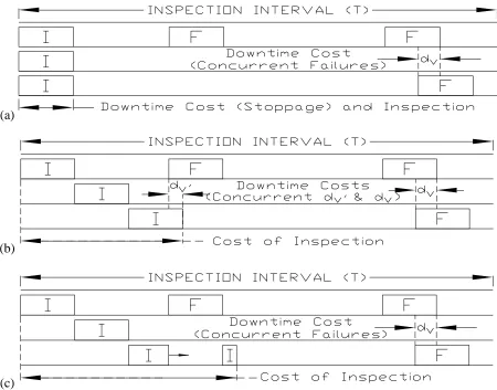
3.5 Policy schematic for two-out-of-three line system (inspection I;
failure repair F; concurrent occurrence of two failure stoppages 𝑑𝑣; concurrent occurrence of a failure stoppage and an inspection 𝑑𝑣′):
3.6 The base model for the single-line
packing facility, showing eight programming algorithms --- 61
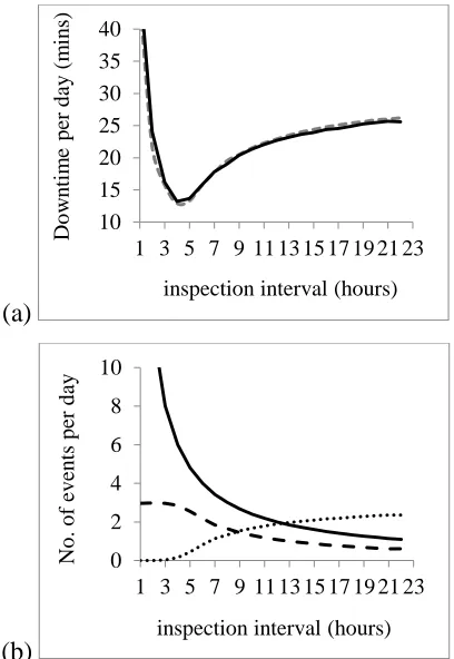
3.7 Comparison of results for the single-line packing system:
(a) expected downtime per day against preventive inspection interval; and
(b) expected number of events against preventive inspection interval --- 62
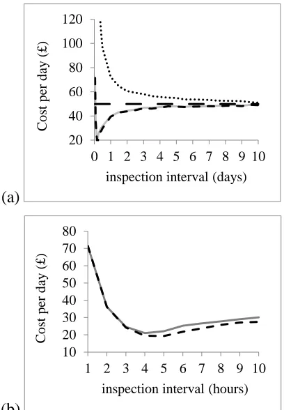
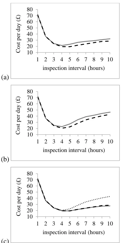
3.8 Cost-rate as a function of inspection interval: (a) all policies
with inspection interval up to 10 days; and (b) consecutive policies only --- 64
3.9 Cost-rate as a function of inspection interval:
(a) standard two-out-of-three parallel system; (b) three-line system;
and (c) consecutive inspection prioritising failure repair for each system --- 66
3.10 Sensitivity analysis of parameters: (a) inspection duration;
(b) failure stoppage duration; and (c) defect arrival intensity --- 68
Figures associated with Chapter 4
4.1 Defect arrivals and failure occurrences
in this complex system of multiple components --- 78
4.2 Characteristics of the periodic and
continuous review inventory replenishment policies --- 80
4.3 The effect of different inventory
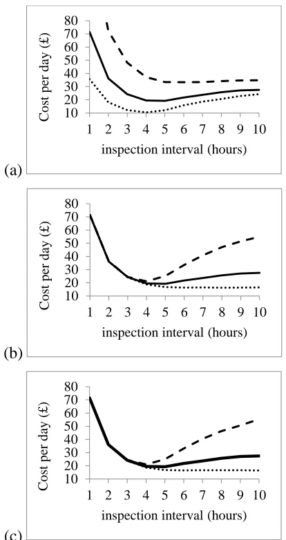
replenishment policies on the joint optimisation cost --- 86
4.4 For the optimum policy in each class of inventory policies:
(a) order cost-rate; (b) order point statistics; (c) holding cost-rate;
(d) PM statistics; (e) stock-out cost-rate; (f) order size statistics;
(g) failure rate; and (h) maintenance cost-rates --- 90
4.5 The sensitivity on the joint optimisation cost for the optimal
(𝑅, 𝑆, 𝑇 = 2𝑅) policy for various parameters (x=minimum; *=baseline):
(a) defect arrival rate; (b) failure delay-time; (c) cost-rate of machine downtime;
(d) inspection cost; (e) unit cost; (f) ordering cost; (g) shortage shipment cost; and
5.1 Defect arrivals, failures, failure stoppage duration F, and
replacement stoppage duration R in this complex system of
multiple components for a two-machine (MC1 & MC2) parallel system --- 104
5.2 Characteristics of the (𝑅, 𝑆) inventory control policy using standard ordering ---- 107
5.3 Flowchart of the general simulation procedure,
showing the flow of entities from one modelling routine to another --- 111
5.4 Flowchart of the Clock (planned/scheduled)
downtime routine for each machine --- 113
5.5 Flowchart of the Clock (planned/scheduled)
downtime sub-processes 1, 2 & 6 routines for each machine --- 114
5.6 Flowchart of the Clock (planned/scheduled)
downtime sub-processes 3, 4 & 5 routines for each machine --- 115
5.7 Flowchart of the CalculateTimeCostMCS subroutine (multi-line) --- 117
5.8 Flowchart, depicting the process of capturing
and recording simultaneous machine downtime --- 120
5.9 Joint maintenance-inventory policy variants
considered under: a) standard; and b) just-in-time ordering --- 122
5.10 The effect on the joint optimisation cost:
(a) the best four-out-of-ten policy variants (optimal policy*;
optimum intervalX); and (b) order-up-to-level S for T=5 (weeks) --- 124 5.11 For the best four-out-of-ten joint policy variants
(optimum policy*): (a) defect removal rate;
(b) failure rate; and (c) defect/failure statistics at optimum interval --- 126
5.12 For the best four-out-of-ten joint policy variants (optimum policy*): (a) inspection rate; (b) positive inspection rate; and
(c) inspection/spares statisticsat optimum interval--- 127
5.13 For the best four-out-of-ten joint policy variants (optimum policy*): (a) maintenance cost-ratesresults at optimum interval; and
at optimum interval (optimum policy ):
(a) ordering cost-rate; (b) holding cost-rate;
(c) simultaneous machine downtime cost-rate; and
(d) stock-out cost-rate --- 130
5.15 For the best four-out-of-ten joint policy variants (optimum policy*): (a) order opportunity rate; (b) order placing rate;
(c) mean order size; and (d) maximum order size --- 131
5.16 The effect of various parameters on the cost-optimal policy
(*baseline): (a) defect arrival rate; and (b) failure delay-time --- 133 5.17 The effect of various parameters on the cost-optimal policy (*baseline): (a)
List of Appendices
Appendices associated with Chapter 1
1.1 Developing a simple model using the ProModel simulation tool --- 146
Appendices associated with Chapter 2 None. Appendices associated with Chapter 3 3.1 A summary of the modelling framework specifically for the modified two-out-of-three parallel system with consecutive inspection prioritising failure repair --- 154
3.2 On-screen layout of simulation model --- 158
3.3 Percentage time packing lines are either working or idle, under the modified 2-out-of-3 parallel system --- 159
3.4 Average number of defects arriving at packing line 1 --- 159
3.5 Detailed source data for the single-line packing system --- 160
3.6 Detailed source data for the modified two-out-of-three parallel system --- 160
Appendices associated with Chapter 4 4.1 Survey questionnaire: (a) Collecting data from maintenance experts and paper machine manufacturers --- 161
(b) Survey response values --- 162
4.2 Flowchart of the general simulation procedure, showing the flow of entities from one modelling routine to another --- 163
4.3 Determination of the simulation warm-up period using:
(a) the Time Series method; (b) Welch’s method; and
4.4 A sample analysis for the determination of number of replications --- 165
4.5 On-screen layout of simulation model --- 166
Appendices associated with Chapter 5 5.1 Flowchart of the general simulation procedure, showing the flow of entities from one modelling routine to another --- 167
5.2 Details of the model: (a) locations; and (b) entities --- 168
5.3 Flowchart of the Clock (planned/scheduled) downtime routine for each machine --- 169
5.4 Flowchart of the Clock (planned/scheduled) downtime sub-processes 1, 2 & 6 routines for each machine --- 170
5.5 Flowchart of the Clock (planned/scheduled) downtime sub-processes 3, 4 & 5 routines for each machine --- 171
5.6 Flowchart of the Called (unplanned/unscheduled) downtime routine for each machine --- 172
5.7 Flowchart of the Called (unplanned/unscheduled) downtime sub-processes routine for each machine --- 173
5.8 Details of the model: (a) resources; (b) processing; and (c) arrivals --- 174
5.9 Flowchart of the Processing Operations routine for the Machine Process to Downstream Process and Exit --- 176
5.10 Flowchart of the Processing Operations routine for the Defect Arrival to Failure Occurrence --- 177
5.11 Flowchart of the Processing Operations routine for the Failure Occurrence to Exit --- 178
5.12 Flowchart of the Processing Operations routine for the Failure Occurrence to Defect Dump & Exit --- 179
5.13 Details of the model: (a) attributes; (b) macros; and (c) subroutines --- 180
5.14 Flowchart of the CalculateTimeCost subroutine (individual machines) --- 181
5.15 Flowchart of the OrderSparesMCS subroutine --- 182
and recording simultaneous machine downtime --- 184
5.18 On-screen layout of simulation model --- 185
5.19 SimRunner screen-captures: inputting model parameter values
List of Abbreviations
CM Corrective Maintenance
PM Preventive Maintenance
CBM Condition-Based Maintenance
DTM Delay-Time Modelling
DES Discrete-Event simulation
SKU Stock-Keeping Unit
Chapter 1
Introduction
1.1. Background and methodology
Many research papers have been published during the past decades contributing to the
ever-growing interest in using maintenance analysis in the area of Production and Operations
Management, and to guide the decision-making process (Wang, 2012a). In particular, the issue
of equipment downtime and the need for the reduction of its associated costs including spare
parts inventory, has been the subject of intense research.
Imagine a plant with one or more failure modes, which has a maintenance policy of repairing failures as they arise and inspecting every 𝑇 time units. The objective of the inspection would
be to identify and remove any defects before they cause machine failure. Clearly, in this context,
the aim would be to minimise the plant operational downtime by reducing the effects of failures
and inspection stoppages. Therefore, the main decision variable is the optimal inspection
interval, 𝑇. If a short interval is used for 𝑇, the percentage of time that the plant would potentially be operational will be reduced since there would be frequent inspection activities.
Alternatively, if a large 𝑇 is used, then one would not distinguish between this policy and running the plant under a breakdown maintenance regime. There are five factors that would
influence the determination of the optimum inspection interval and thus minimizing the cost of
downtime: (i) the timing and the rate of arrival of defects; (ii) the time it takes for defects to
cause failures; (iii) the pace at which inspections are undertaken; (iv) the cost and downtime
associated with inspections and defect removal (by replacing/repairing parts); and finally (v)
the cost and downtime associated with replacing/repairing failures. Thus, using a modelling tool
Many methodologies have been proposed and several concepts have been developed to test and
establish the optimum inspection interval, which would minimise the expected downtime and
hence the overall cost of production. One of these inspection methodologies is the delay-time
modelling (DTM) concept, which describes the failure of industrial equipment in two separate,
but linked stages. The first stage defines the time lapse between the new (or as new) up to such
a time that a defect arrives - the time-to-defect. The second stage describes the time during which
the defect continuously deteriorates, up to the point where it finally fails - the delay-time. It is
this second stage or delay-time which opens a window of opportunity for the inspection of plant,
identification of defects, and replacement/repair of parts, before downtime occurs.
A number of review papers are present in the literature addressing the issue of optimising the
preventive maintenance interval to maximise the operations of industrial plant. These include
Thomas (1986), Cho and Parlar (1991), Dekker (1996), Wang (2002), Nicolai and Dekker
(2008), Van Horenbeek et al. (2013) and Ding and Kamaruddin (2015). It is noted from these
reviews that most, if not all, analytical models are based on assumptions which simplify real
life situations and make them less practical. In practical situations, simplifying assumptions is
undesirable but permissible to some extent for converging, as far as possible, the application of
theory into practice. To relax or eliminate some assumptions of these models, will make them
less practical to be implemented. Scarf (1997) is an “appeal to maintenance modellers to work
with maintenance engineers and managers on real problems”. The author acknowledges, “too
much attention is paid to the invention of new models, with little thought, it seems, as to their
applicability”. It is interesting to note that the same observation still seems valid since evidence
suggests that little research is conducted on the optimisation of maintenance in industrial
systems (Alrabghi et al., 2017).
For certain industrial situations such as multi-line settings, developing analytical models might
prove intractable or mathematically untraceable. The other avenue, which is followed in this
In developing the simulation models in this thesis, ProModel (ProModel, 2016), a process-based
discrete-event simulation language, (see for example, Harrell et al., 2011), one of many
proprietary simulation packages available in the market, was used (see Appendix 1.1, for the
procedure to develop a simple model using ProModel). The models, composed of 𝑛 machines (𝑛 ≥ 1), were developed as continuous production lines. To ensure that the optimal
cost is achieved, SimRunner (see ProModel, 2010), a simulation optimisation tool, is integrated
with the simulation models, which performs sophisticated analysis to determine the optimal
value of decision variable(s). The optimisation tool automatically runs multiple combinations
of certain variables (if needed) to find the unique combination, which provides the optimal value
of the objective function - the long-run average expected cost (or cost-rate). When optimising a
particular system, one might use either exact solution methods (analytical) or heuristic methods
to find near optimal values for the decision variables. Safety factors, environmental impact,
various service levels, system downtime or costs, to mention only a few, are examples which
could be used as a focus in an optimisation study. The minimisation of the costs is most common
in the optimisation of maintenance-inventory problems (Van Horenbeek et al., 2010), which is
also used for the models in this thesis. An optimisation study of a different context is the joint
age-usage maintenance strategy by Shafiee et al. (2016) applied to railway tracks, for which the
maintenance cost-rate is also minimised.
1.2. Aims and objectives
The main aim of this research is to develop simulation models in order to jointly optimise
preventive maintenance and spare part provisioning for multi-line production systems. This is
in order to eliminate, or at least to minimise, the occurrence of simultaneous downtime in
systems where there are parallel production machines. Simultaneous machine downtime may
halt production, which will have a significant adverse effect on profitability or other
performance measures. The research uses contexts for which analytical models cannot be
developed due to the underlying difficulty in mathematical analysis and intractability. The aim
To undertake a comprehensive literature review of maintenance methodologies and
policies for determining the optimum inspection interval for different production line
configurations – measured by searching through published and review papers and key
literature on maintenance optimisation using analytical and simulation models, and
compiling a comprehensive literature;
To develop discrete-event simulation models for multi-line production systems, and for
the interface between maintenance and production management activities – measured
by developing working simulation models, the results of which are optimised by the use
of an optimisation tool;
To make recommendations for practitioners to manage effectively the maintenance of
their industrial plant – measured by producing a set of results and performance measures,
to compare and contrast the key differences and characteristics of each policy;
To assess the viability of the proposed models in real-world situations – measured by
applying the simulation models to: (i) real-life case studies, (ii) reported case-studies in
the literature; and finally (iii) idealised contexts documented in journal papers;
To develop solution tools for gaps identified in the literature and make a significant
contribution – measured by demonstrating and presenting findings at conferences and
publishing papers in journals on the joint modelling and simultaneous optimisation of
1.3. Structure of this thesis
This chapter described the background information for helping to understand matters which will
be discussed in more detail in the subsequent chapters. It also described the simulation
methodology used in this PhD thesis. Chapter 2 reviews the general literature on three important
topics of maintenance systems (including delay-time modelling), inventory control systems, and
discrete-event simulation, all of which are pertinent to the topic of this thesis. However, more
specific literature review is presented in each of the three principal Chapters, 3 to 5. Chapter 3
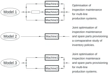
discusses in detail, the optimisation of preventive maintenance for a multi-line production
system in the context of a case study by developing a number of simulation models (model 1 in
Figure 1.1). In Chapter 4, a single-line production plant provides a real context for jointly
optimising the planned maintenance of a paper making machine and the associated spare part
inventory using the delay-time concept and a number of spare replenishment policies (model 2
in Figure 1.1). The detailed discussion in this chapter gives insights into the characteristics of
each policy considered. Chapter 5 describes the development of several simulation models
which aim to jointly optimise the planned maintenance and spare part provisioning for an
industrial plant comprising a two-machine parallel system (model 3 in Figure 1.1). Chapter 6
summarises the findings and conclusions of the work carried out in this PhD. In addition, it
describes the proposed extensions to the simulation models already developed. Detailed
appendices related to various simulation models described in Chapters 3 to 5, and the list of
Figure 1.1. The schematic diagram of production configurations
used in developing the three sets of simulation models in Chapters 3, 4 and 5:
Model 1 Chapter 3 Data from Akbarov et al. (2008);
Model 2 Chapter 4 Data from survey and Wang (2012b);
Model 3 Chapter 5 Data from survey and Wang (2012b).
Machine1
Optimisation of
inspection maintenance for multi-line
production systems.
Joint optimisation of inspection maintenance and spare parts provisioning: a comaparative study of inventory policies.
Joint optimisation of inspection maintenace and spare parts provisioning for multi-line
production systems.
Model 1
Model 2
Model 3
Machine2
Machine3
Machine1
Machine1
Chapter 2
Literature review and Notation
This chapter presents the general literature review on three important topics of maintenance,
inventory control, and discrete-event simulation. However, more specific literature is reviewed
in each of the three principal Chapters, 3 to 5.
2.1. Maintenance systems
Over the past half a century, many review papers have appeared in the maintenance literature
including: McCall (1965); Thomas et al. (1991); Cho and Parlar (1991); Dekker (1996); Dekker
and Scarf (1998); Wang (2002); Pierskalla and Voelker (2006); Nicolai and Dekker (2008);
Pophaley and Vyas (2010); Das and Sarmah (2010); and Van Herenbeek (2013). For many
years, mathematical models have been used for quantifying maintenance functions of industrial
plant using various optimisation techniques (Pierskalla and Voelker, 2006). The primary
purpose of maintenance optimisation is to find an effective implementation of maintenance
policies to minimise maintenance costs or system downtime, or maximise system availability,
to mention only a few examples for the focus in the objective function. Maintenance models, if
developed appropriately and applied correctly under prescribed conditions, can prove to be very
cost-effective in practice (Wang, 2012a).
When a system is to be maintained or restored, the consequence of the maintenance actions
undertaken can result in different outcomes. Pham and Wang (1996) give a comprehensive
Perfect maintenance - after the maintenance actions are carried out, the fixed system is as
good as new.
Imperfect - the system is restored to a state between as good as new and as bad as old.
Minimal - the system is restored to an as bad as old state with the same failure rate as before.
Worse - the system’s condition is worse than just before the maintenance actions were
undertaken.
Worst - the system breaks down completely after the maintenance actions are carried out.
Some of the terminologies used here may also apply to the replacement of parts. Perfect
replacement, as opposed to repair, may occur if the correct parts are installed and the system’s
state is restored to as good as new. Conversely, replacements can be imperfect if the wrong
installation of parts have taken place. The perfect and imperfect analogy may also be applied to
inspection. If all faults or defects are identified at an inspection, the inspection is said to be
perfect, and anything less is thus imperfect. Van Horenbeek et al. (2013) state that the vast
majority of the papers in the literature assume perfect inspection for the restoration of their
systems. The authors give a detailed account of the three main maintenance strategies, namely:
(i) corrective; (ii) preventive; and (iii) predictive maintenance. Wang (2002) also reviews the
most important preventive maintenance policies for both single and multi-unit systems. It
should be noted that, a part or a component of a machine (or equipment) is called a unit, which
may be repaired or replaced upon failure, or identified as defective and repaired/replaced at
inspection. The three terms: unit; part; or component are used interchangeably by different
authors.
Under the corrective maintenance, or sometimes referred to as failure-based maintenance,
whenever a unit fails, it is immediately repaired or replaced by a new one, provided spares are
available. Consequently, if no spare is available, equipment downtime will normally occur and
In the manufacturing sector, for example, bearings used extensively in a production plant can
fail unexpectedly and catastrophically (Folger et al., 2014a; 2014b) which will need to be
repaired or replaced. In other situations, unexpected failure of components may cause disruption
to services or accidents (Dinmohammadi et al., 2016). Corrective maintenance is the most
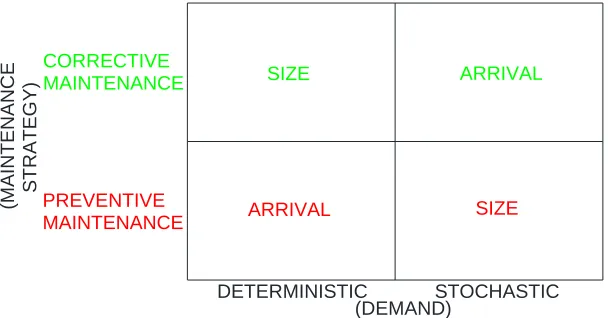
reactive of all maintenance strategies. Figure 2.1 illustrates that as corrective maintenance is not
planned, the demand requirements (the arrival of defects) is stochastic, yet its size is
[image:27.612.150.454.230.389.2]deterministic (normally single-units) (Wang and Syntetos, 2011).
Figure 2.1. Demand behaviour of and spare part requirements
under corrective and preventive maintenance strategies.
Systems may also be maintained under a preventive strategy where equipment is inspected at
regular intervals, with a view to identifying and replacing all defective (faulty) parts before they
cause failures (for example, Wang, 2008). Evidently, there is a strong link between the
preventive maintenance inspection interval and the spare part inventory. If the inspection
interval is too short, then the ‘lumpy’ demand effect is created. This is the result of replacing
multiple defective but still working parts to reduce the risk of failure at a later stage. Equally, if
the inspection interval is too long, then the number of single-unit parts randomly failing is
increased, adding to the overall downtime. As shown in Figure 2.1, the timing of preventive
maintenance, by its nature, is deterministic as it is planned in advance. However, under this
policy, although the demand for spare parts is deterministic, its size is stochastic. There are a
number of major policies that fall under this category which may be implemented depending on
whether the system under consideration is single or multi-unit. If the asset, machine or
(DEMAND)
PREVENTIVE MAINTENANCE
CORRECTIVE
MAINTENANCE ARRIVAL
ARRIVAL
SIZE
SIZE
DETERMINISTIC STOCHASTIC
(M
AIN
TEN
ANCE
STR
equipment lends itself to being maintained based on the age of the unit, then the well-known
age-based preventive maintenance, first suggested by Barlow and Hunter (1960), may be used.
Under this policy, apart from the units that have failed in service, the rest are replaced whenever
they reach their predefined age. Sequential maintenance may also be considered as age-based
preventive maintenance since the frequency of maintenance will be increased as the machine
and/or units become older. In comparison, under the periodic block-based strategy, failed units
are replaced too, but all units are also ‘block-replaced’ at constant intervals regardless of their
history, current condition, and age. Finally, under the failure limit policy, units are replaced
when the failure reaches a predetermined rate. Units may or may not be independent or identical.
In systems where multiple units exist, parts may be maintained using group or opportunistic
strategies. The group maintenance policy combines the same features of the age-based and
block-based strategies described for the single-unit systems but as a group replacements for
multiple unit of parts. If dependencies exist between the units, one could ‘opportunistically’
replace other units when a failure occurs. It is important to note that under all policies, failed
units are immediately replaced by new ones provided spares are available.
Finally, under the predictive maintenance strategy, better known as condition-based
maintenance (CBM), the state of the system is continuously observed and monitored, and where
certain or a combination of ‘signals’ such as product quality, tolerances, excessive vibration,
heat, odour, noise etc., reach a prescribed limit, maintenance action is undertaken and units may
be replaced (for example, Shafiee et al., 2015). CBM was introduced in order to ensure that PM
is only triggered when required, either through scheduled inspections or with smart assistance
of sensors, providing data for specialised maintenance software (see, Olde Keizer et al., 2017
for the latest review paper).
Whichever maintenance strategy is used to restore the system under consideration, different
costs will be incurred. These costs could include inspection, downtime, labour and spare
replacements, for example. A distinction must also be made between failure replacement and
preventive replacement, which will have a different cost element for the associated labour and
Alrabghi and Tiwari (2015) observe that the vast majority of journal papers in the maintenance
literature, make use of only a limited number of maintenance strategies and policies rather than
comparing different alternatives for particular contexts. They conclude that the research in the
literature is also limited in terms of comparing and selecting the optimum maintenance policies
in multi-component systems.
2.1.1. Delay-time modelling
Delay-time modelling (DTM) was first introduced by Christer (1976) in the context of building
maintenance. It was eight years later when Christer and Waller (1984a) applied the same
concept to an industrial maintenance problem. Since then, many research papers have appeared
in the literature with regard to the concept of this methodology and many more have been
published to describe several industrial applications. Since its conception in 1976, a few detailed
review papers have been published on delay-time modelling, by Baker and Christer (1994),
Christer (1999) and Wang (2012a). Also, a textbook chapter by Wang (2008) comprehensively
discusses different aspects of the methodology.
Delay-time modelling, describes the evolution of defects in industrial equipment in two separate
but linked stages, as illustrated in Figure 2.2. The first stage is the time lapse from new (or as
new) until a defect (or fault) arrives. This is the time-to-defect arrival, 𝑢. Equivalently, it is the
sojourn in the good state. The second stage is the time lapse from defect arrival to the point at
which this defect causes the equipment to fail. This is the delay-time, ℎ. Equivalently, it is the
sojourn in the defective state. The second stage opens a window of opportunity for inspection, identification of defects, and remedial maintenance intervention (component repair or
replacement) before a defect causes failure. By the definition of the delay-time, the plant state
before failure is binary: good or defective (Wang, 2012a). Thus, the ‘change point’ from the
good state to the defective state occurs at a random time, failure occurs some random time later,
and the time of transition from the good to defective state is only observable by inspection. By
time-to-defect and delay-time may be estimated, and the relationship between the number of
failures and the inspection interval can be established, as discussed by Baker and Wang (1992).
Figure 2.2. The delay-time concept.
In modelling a system, if 𝜆 denotes the rate of arrival of defects from all components within an industrial plant, and 𝐹(ℎ) denotes the delay-time distribution of all failures, then the expected number of failures, 𝐸𝑁𝑓(𝑇), within an inspection interval 𝑡 (over 0, 𝑇), is given by (Christer and Waller, 1984a):
T
f T F hdh
EN
0
) ( )
(
--- (1)
The above formula is derived under a perfect inspection assumption, and it is the fundamental
expression used in all delay-time-based models. This formula explicitly establishes the desired
relationship between the expected number of failures and the inspection interval. The probability, 𝑏(𝑇), that a fault arising causes a failure is:
𝑏(𝑇) =𝐸[𝑁𝜆𝑇𝑓(𝑇)] --- (2)
(Christer, 1999), which increases from 0 to 1 as 𝑇 increases from 0 to ∞. Accepting the following basic delay-time-modelling assumptions: (i) the plant is running under steady-state
Poisson process (HPP); (iii) all defects are identified at inspection, every 𝑇 time units, and 𝑑𝑠<<
𝑇; and finally (iv) failures are repaired/replaced immediately; then the expected number of failures over an inspection period is 𝜆𝑇. 𝑏(𝑇), and the expected downtime per unit time 𝐷(𝑇)
becomes:
𝐷(𝑇) =𝑑𝑓.𝐸[ 𝑁𝑓((𝑖−1)𝑇,𝑇)]+𝑑𝑠
𝑇+ 𝑑𝑠 =
𝑑𝑓.λT.b(T)+𝑑𝑠
𝑇+ 𝑑𝑠 --- (3)
(Christer and Wang, 1995). These expressions clearly exhibit the expected characteristics of
having large values for small 𝑇, and where 𝑑𝑓 is the mean downtime per failure and 𝑑𝑠 is the mean downtime per inspection. Equation (3) can be minimised in terms of, 𝑡 if the expected
number of failures can be computed and 𝑑𝑓 and 𝑑𝑠 are known. Equation (3) is established assuming that the defects identified at an inspection will always be removed without costing
any extra downtime or cost. This assumption can be relaxed as shown in equation (4) below
(Wang, 2008):
𝐷(𝑇) =𝑑𝑓.𝐸[ 𝑁𝑓((𝑖−1)𝑇,𝑇)]+𝑑𝑠+𝑑𝑟.𝐸[ 𝑁𝑟(𝑖𝑇)]
𝑇+ 𝑑𝑠+ 𝑑𝑟.𝐸[ 𝑁𝑟(𝑖𝑇)] --- (4)
Clearly, the form of distributions regarding the failure time and the associated parameters must
be selected and estimated. Christer and Waller (1984a) state that, when a defect is identified at
an inspection, the following questions may be asked: how long ago (HLA) could an inspection
or operator have first noticed the fault? And, if the defect is not removed, how much longer
(HML) could it be delayed before it causes downtime? The delay time for each fault is then
estimated by ℎ = 𝐻𝐿𝐴 + 𝐻𝑀𝐿. In this way, by observing sufficient defects, a prior distribution
for 𝐹(ℎ) may be obtained. And, if the inspection identifying a defect is made at time 𝑡, then 𝑢 = 𝑡 − 𝐻𝐿𝐴.
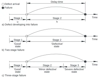
Wang (2011b) extended the delay-time concept from a two-stage (Figures 2.3 (a) and 2.3(b))
into a three-stage (Figure 2.3(c)) failure process, where the delay-time stage is divided into two
stages, corresponding to a minor and a severe defective stage. This means that, at any one time,
failed. The three-stage delay-time concept seems to better reflect the true states of a plant item
in reality, however, the extended model is more complicated to develop and will require more
information to enable the parameter estimation procedure in practice (for example, Baker and
[image:32.612.150.471.184.435.2]Wang, 1992).
Figure 2.3. A depiction of development of the three-stage delay-time model.
Delay-time modelling captures the relationship between failures of items in service, inspection
at constant PM epochs, and PM replacement of defective items under the assumption that all
defective items are always identified and replaced (provided spares are available) at inspections.
The fundamental difference between DTM and other inspection strategies is that under the
former, only defective items (if any) are replaced at inspection intervals. In comparison, under
the age-based policy, items are only replaced according to their age, or irrespective of their age
and condition under the block-based replacement policy. Apart from inspection, and
repair/replacement at PM interventions and failure events, there may be other activities, such
as, removing metal burrs, lubricating components, and changing engine oil, for example.
Depending on circumstances and if necessary, these events may be modelled using a variable
rate for entity arrivals.
u h
Time
a) Defect developing into failure Defect arrival
Failure
Stage 1 Stage 2
Time
b) Two-stage failure Stage 1
'Good' state
Stage 2 'Defective'
state Delay-time
Time
c) Three-stage failure Stage 1
'Good' state
Stage 2 'Minor defective'
state
Stage 3 'Severe defective'
DTM is a modelling methodology that can be used to determine an inspection-based or
block-based PM policy, where all items are inspected at constant inspection intervals (a decision
variable to be determined) and defective items are ‘block’ replaced. Under an inspection or
block-based PM policy, inspection identifies all defective items that will be replaced, whereas
in a normal block-based replacement policy all items are replaced regardless of their age and
conditions. Generally, failures of the items in service generate intermittent single-unit demand.
In addition, the inspection process generates multiple (lumpy) demand as a result of identifying
and replacing all defective items at PM intervals. Furthermore, the timing of demand for spare
parts is stochastic at failures, but deterministic at the times of preventive replacements.
There are two distinct types of DTM systems: (i) single-component or component tracking; and
(ii) multi-component or complex system. In a single-component system, as shown in Figure 2.4,
there may be a single dominant failure mode, and the system may be renewed upon failure
(Wang, 2008). Under the inspection-based policy and the instance shown in Figure 2.4,
inspection at the first and third epochs will identify and remove the defects and the system is
thus renewed. However, before the 2nd and 4th inspection epochs, component failures occur and the system is renewed again upon replacements. Examples of single-component systems are
reported in: Baker and Wang (1992, 1993); Wang and Christer (1997); and Yang et al. (2016).
Figure 2.4. Defect arrivals and failure occurrences in a single-component system.
In contrast, a complex system is one in which many failure modes could arise, and the correction
of one failure or the replacement of one defect will have nominal impact upon the overall plant Corrective
Preventive
T T T T
Maintenance
Maintenance
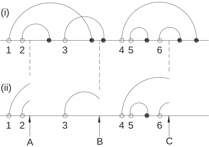
failure characteristics or the steady state of the system. Figure 2.5(i) depicts an example of a
complex system where six defects (1, 2, etc.) arrive over time. With the assumption of perfect
inspection, if regular inspection takes place, for example at points A, B and C, then some defects
will be identified and removed before failures occur, as shown in Figure 2.5(ii). Considering
Figure 2.5(ii) further, at inspection point A, two defects have already arrived and are currently
in their delay-times. Thus, both defects 1 and 2 will be identified and removed at inspection
point A, either by replacing or repairing before failures occur. Defect 3 arrives in the middle of
the period between scheduled inspections A and B and will be identified and removed at
inspection point B. Before inspection C, one failure occurs as a result of defect 5. However the
inspection at point C, identifies and removes both defects 4 & 6 before they cause downtime.
Therefore, in this instance, with a suitable length for the inspection interval, 5 out of 6 defects
(83%) will be identified and removed. The system may thus be renewed at inspection points A,
B and C if the rate of arrival of defects is constant and the inspections are perfect. Most
delay-time-based models reported in the literature are models of complex systems, and examples
include: Christer and Waller (1984a, 1984b); Christer et al. (1995); Akbarov et al. (2008); Jones
et al. (2010); Lu and Wang (2011); and Pietruczuk and Werbinska-Wojciechowska (2017).
There are many delay-time-based case study applications reported in the literature. Some
examples include: Christer and Waller (1984a); Christer (1987); Baker and Wang (1992, 1993);
Christer et al. (1995); Pillay et al. (2001a, 2001b), Arthur (2005); Akaborov et al. (2008); Jones
Figure 2.5. Defect arrivals and failure occurrences
in a complex system of multiple components.
2.2. Inventory control systems
Maintenance costs are clearly dependent on the availability of spare parts. However, many
models assume there is an infinite inventory of spare parts at all times, which makes their use
unrealistic in practice. The inventory for spare parts is normally controlled by a particular
replenishment policy. The overall objective is always to find the optimal policy. Keeping too
many spares will increase the holding cost, which will have financial implications on the
company’s cash flow and/or borrowing, or will increase the risk of spare parts’ obsolescence. Conversely, keeping too few parts might result in the plant’s unavailability at critical times. The
cost associated with the unavailability of spare parts is twofold: (i) the cost of equipment
downtime while awaiting spare delivery; and (ii) the cost of expediting the delivery of parts in
emergencies.
For spare parts classification, the usual approach is to categorise according to a part’s service criticality. “Alternatively, an ABC classification is used, which lists all stock-keeping units
1 2
3
4 5
6
(i)
1 2
3
4 5
6
A
B
C
(SKU) in descending order, by total volume, or total value of sales, with the A items being
assumed to be the most critical and requiring the highest service levels” (Boylan and Syntetos,
2010). However, the process may be guided by criticality and cost considerations, as well as the
ABC classification. Molenaers et al. (2012), classified spares based on attributes like demand
pattern, unit price and inventory costs. Later, Hu et al. (2017) classified spare parts based on
multiple criteria of criticality, price, demand, lead time, and obsolescence, since they noted that
“single objective of price is generally misleading”. The authors state that their approach does
not offer optimisation, but they intend to add this extension as an enhancement in the future.
There are two distinct approaches for the replenishment and management of spare parts (see,
for example, Muller, 2011). Stock may be reviewed: (i) periodically; or (ii) continuously (See,
Kennedy et al., 2002, and Santos and Bispo, 2016, for example). Under the periodic review policy, there are at least three methods by which parts may be replenished: (i) periodically (𝑅), at the beginning of each cycle, raising the inventory position to a pre-defined level 𝑆, based on
the forecasted demand for the next period for example - the (𝑅, 𝑆) policy; (ii) periodically raising the inventory position to level 𝑆 if the stock level has reached or dropped below a certain level 𝑠 - the (𝑅, 𝑠, 𝑆) policy; and (iii) periodically raising the inventory position by ordering a
fixed quantity 𝑄 of stock if the inventory position has reached or dropped below 𝑠 – the (𝑅, 𝑠, 𝑄) policy (see, for example, Silver et al., 2016).
In comparison, under the continuous review policy, every time the stock level is depleted, the
inventory levels are checked. Then, either a sufficient quantity, up-to-level 𝑆 is ordered if the inventory position reaches or drops below 𝑠 – the (𝑠, 𝑆) policy, or a fixed quantity of parts is ordered when the inventory position reaches or drops below 𝑠 – the (𝑠, 𝑄) policy. When there is a per unit demand, both the (𝑠, 𝑆) and (𝑠, 𝑄) policies give the same result when 𝑄 = 𝑆 − 𝑠. A special case of the (𝑠, 𝑄) replenishment policy is famously called a two-bin policy where a
replenishment order, sufficient to fill up the bin, is immediately placed when the first bin is
empty. The second bin is then used during the replenishment lead-time. This policy is mainly
There are three major costs associated with all stock ordering policies, namely: (i) ordering; (ii)
holding; and (iii) shortage costs. Firstly, the fixed ordering cost is either for the unit purchase
cost under normal circumstances or for the replenishment of parts in emergencies. Secondly,
holding inventory is expensive since it will have capital and space cost implications. And
finally, shortage costs will be incurred if the number of spares in stores is insufficient to meet
the demand. Different policies aim to balance these costs in order to produce an overall optimum
cost. Stock replenishment quantities depend on whether the system under consideration is single
or multi-unit. However, when failure frequencies are high or spare replenishment lead-time is
long, it might prove wise to keep more than one part in stock, even for a single-unit system. On
the other hand, keeping multiple units of spare parts increases the cost of inventory and the risk
of obsolescence, which is a major issue and has cost implications too.
2.3. Discrete-event simulation
Simulation has been used for many years to understand and experiment with systems under
study, especially in the production and manufacturing industry where the use of discrete-event
simulation (DES) has been very effective. The use of simulation has grown dramatically since
modern manufacturing systems have become more complex as a result of dependencies and
interactions between system components. Gupta and Lawsirirat (2006) highlight the fact that
the term component has a different meaning in different contexts. Since it is not possible to
model every part in a complex system, it is practical to consider only the components that have
significant impact on the performance of the system. Compared to the traditional and
mainstream discrete-event simulation, agent-based modelling and simulation (ABMS) is a
relatively new technique for simulation (Macal, 2016), for which the number and breadth of
applications has had a huge expansion during the past 10 years (Cheng et al., 2016). A very
important step forward in the world of simulation is the obvious and essential procedures for
verification and validation, which can only lead to credibility of simulation models and the
results achieved from them (Rabe and Dross, 2015). The gap between research in optimization
via simulation and the development of algorithms that can be applied to real-life problems has
use of parallel simulation, which is becoming easy to do, and any simulation study that requires
multiple replications or multiple scenarios will benefit from this advancement (Nelson, 2016).
During the past three decades, simulation software packages or tools have gradually replaced
simulation languages. Dias et al. (2016) ranked the top worldwide most popular and used
simulation software, based on intensity of usage or level of presence in different sources -
“popularity”. The survey findings clearly identify Arena software package as the most ‘popular’
and widely used discrete-event simulation tool, followed by ProModel, which is the tool used
for the development of simulation models in this thesis. The next three most used tools, namely
FlexSim, Simul8, and WITNESS, making up the first cluster, have more or less similar rankings
in the comparison table. It is important to note that the contexts of these simulation tools are
constantly changing, whether in industry or academia, and the ranking may indeed change in
the next survey published in the literature.
Simulation delivers an advantage over analytical approaches since many maintenance policies
are not analytically traceable (Nicolai & Dekker, 2008). Analytical and mathematical
approaches are limited in solving such complex maintenance problems.
To optimise their maintenance problem, Allaoui and Artiba (2004) preferred the use of
simulation over the analytical approach and stated that the immediate availability of
maintenance resources is a major assumption in many studies. Similar conclusions were reached
by Rezg et al. (2005) who used both analytical and simulation approaches (using ProModel) to
develop a model of a system with storage buffers, which helped in reducing the effect of lower
production rate while maintenance interventions were taking place. Gharbi and Kenné (2005)
developed a discrete-event simulation (DES) model in which the degradation of the machine
was modelled as a continuous process to reflect the reality that as time goes by machines are
automatically aged (see also, Roy et al., 2016).
Many authors use discrete-event simulation packages for their maintenance studies. However,
others including Cavory et al. (2001) used a general-purpose programming language to develop
context was difficult and thus used simulation for the resolution of their problem. Ilgin and
Tunali (2007) developed a simulation optimization model, which they believed, gives the ability
to describe multivariate non-linear relations that is difficult to express in an analytical form.
They concluded that a 53% reduction in total annual maintenance cost and 6% improvement in
average monthly production were achieved.
Alrabghi and Tiwari (2015) surveyed the literature and reported on the state-of-the-art
simulation-based maintenance optimisation, which resulted in 59 journal papers since the year
2000. Discrete-event simulation is the most reported technique for modelling maintenance
systems. In comparison with general-purpose languages, specialised simulation software
provide several advantages such as, rapid modelling, animation, automatically collected
performance measures, and statistical analysis tools (Banks, 2010).
Minimising cost is reported as an objective in the majority of simulation studies in the literature.
Kuntz et al. (2001) used an inspection-based model and included machine downtime in the cost
function. Instead of minimising maintenance cost, Roux et al. (2013) argue that maximising
machines’ availability should be the objective function since production costs tend to be higher.
However, other authors believe that the significance of maintenance costs cannot be
underestimated. The use of PM and CBM were investigated in a study by Xiang et al. (2012).
They observe that as sensors get less expensive, the use of CBM strategy will become more
popular, which has potential cost-savings.
The main assumptions common in the majority of simulation-based studies in the literature
include: (i) perfect maintenance in maintaining identical and independent units; (ii) failures are
detected immediately; (iii) costs of maintenance actions are constant, but the cost of CM is
always higher than PM; (iv) duration of maintenance activities are constant or take zero time;
and finally, maintenance resources are always immediately available when required.
Considering the points listed above highlight the limitations of studies in the literature.
Since it is difficult to obtain accurate cost data for conducting maintenance and inspection
literature, which test the robustness of a suggested model by varying inputs and investigating if
the results are in line with the expected outcome (Boulet et al., 2009). Surprisingly, many
researchers do not disclose the simulation technique or the specific software used in their
research, which will limit the replicability of the experiments by independent researchers.
Over the years, discrete-event process simulation has steadily grown in power due to the
advancement of hardware, ease of application due to software sophistications, availability of
expertise due to the growth of simulation as a business-improvement tool, and breadth of
applications to business challenges, especially in manufacturing. There are different reasons and
motivations for the use of simulation to initiate a manufacturing-context simulation project.
Khalili and Zahedi (2013) used simulation to prepare a mattress production line for anticipated
demand increases over a five-year planning horizon (Williams, 2014). Natarajan (2016) reports
on a simulation-based case study of a production line at an automotive ancillary manufacturing
plant. In the first phase, the existing system is simulated to identify the critical operations in the
system. Then, the existing system is modified based on the suggestions of the finding of the
initial phase of this study. Finally, the revised model is simulated, which produces
improvements in the production volume for the engine thrust bearing line. Rozen and Byrne
(2016) examine preventative maintenance segregation with the aim of determining the optimum
PM frequency that results in reduced cycle time. The resulting solutions from many years of
maintenance modelling have proven to be very effective. However, to improve on those simple
solutions, complex and time-consuming simulation modelling is required, and reliable input
data is even more important, which is driven by Big Data and the Internet of Things technologies
(Volovoi, 2016b). In order to be successful in this path, the inner workings of DES, so far hidden
from decision makers, have to be highlighted to the users (Volovoi, 2016a) (also see, Alrabghi
and Tiwari, 2016).
In many studies, simulation is used as a solution tool. Sarker and Haque (2000) used simulation
since the development of mathematical models was “extremely difficult”. In their model, they
considered maintenance resources, such as spare parts, and concluded that the results of their
optimized policies. Tateyama et al. (2010) is one of few research articles that considers
maintenance resources, such as technicians, as decision variables.
Maintenance plays a key role to sustain the operations of manufacturing systems under high
production throughput, reliability and safety requirements. Opportunistic maintenance gives
staff the chance to replace or repair those items that are found to be defective or need
replacement during the maintenance of another machine or component. However, components
are usually assumed to be independent. Lung et al. (2016) develop an opportunistic maintenance
policy, considering both economic and structural dependence between different components. In
Babishin and Taghipour (2016), a system consisting of components subject to soft and hard
failures is modelled using simulation together with an optimisation tool. Hard failures are
self-announcing and are fixed immediately (similar to failures under DTM) and provide an
opportunity for inspection (opportunistic inspection). Soft failures (which may be thought of as
defects under DTM) are only identified and revealed at periodic inspections, which are then
corrected (repaired or replaced).
A specific application of simulation optimisation is in the area of opportunistic maintenance of
wind farms. Corrective and time-based preventive policies are widely employed for the
maintenance optimisation of wind turbines. In Zhang et al. (2017), an opportunistic maintenance
approach is proposed, considering imperfect maintenance based on reliability. The simulation
results highlight the economic advantage of using an opportunistic maintenance strategy. The
cost of energy generated from offshore wind is dependent on maintenance cost to a great extent,
which in turn depends on the strategy for performing maintenance. In Sarker and Faiz (2016)
model, opportunistic maintenance is performed on other components in the system while a
failed component is replaced. The model in Irawan et al. (2017) aims to optimise the
maintenance schedule, the routes for the crew transfer vessels to service the turbines, and the
number of technicians required for each vessel. The proposed approach was tested using data
from a case study reported in the literature as well as for a context generated randomly. The use
of opportunistic maintenance strategy is becoming very popular in the literature for reducing
the cost of wind power generation. Policies are developed and decisions are made based on