DESIGN AND VALIDATION OF A PID AUTO-TUNING ALGORITHM
Diego F. Sendoya-Losada and Jesús D. Quintero-Polanco
Department of Electronic Engineering, Faculty of Engineering, Surcolombiana University, Neiva, Huila, Colombia E-Mail: [email protected]
ABSTRACT
The purpose of this paper is to present the development of a PID auto-tuner algorithm based on specifications, which is generally valid for several processes. Based on prior art results, the rationale follows the principles of approximating the closed loop response to a second order transfer function. However, it is shown that the derived algorithm is generally valid and can work well on several examples which are much more complex than second order systems.
Keywords: auto-tuning, closed loop control, frequency response, PID.
1. INTRODUCTION
Tuning controllers for optimal closed loop performance depends heavily on the process to be controlled and identification is still a burden for the control engineer and remains a significant time-consuming task. Auto-tuning is a very desirable feature and almost every industrial PID controller provides it nowadays [1,2]. These features provide easy-to-use controller tuning and have proven to be well accepted among process engineers [3].
For the automatic tuning of the PID controllers, several methods have been proposed. Some of these methods are based on identification of one point of the process frequency response, while others are based on the knowledge of some characteristic parameters of the openloop process step response. The identification of a point of the process frequency response can be performed either using a proportional regulator, which brings the closedloop system to the stability boundary, or by a relay forcing the process output to oscillate [4-7]. Usually these preliminary tests are used to determine a model for the process, along with the tuning of controller parameters [8, 9].
This paper presents the design and validation of a generally valid algorithm for a specifications based PID auto-tuner. The next section provides the underlying principles of the proposed algorithm. The third section is a validation of the auto-tuner on two complex systems: i) a second order plus integrator (double integrator in the closed loop) and ii) a first order with integrator, time delay and non-minimum phase dynamics. Furthermore, the conclusions summarize the main outcome of this work.
2. MATERIALS AND METHODS
The development of this auto-tuning algorithm is based on the prior art where two relay-based PID auto-tuners have been presented: the Kaiser-Chiara auto-tuner and the Kaiser-Rajka auto-tuner [10]. Hence the proposed algorithm is an extended combination of the two: the Kaiser-Chiara-Rajka auto-tuner algorithm (KCR).
The approximation of a closed loop response by a dominant second order transfer function with gain one:
= + 𝜁𝜔𝜔𝑛
𝑛 + 𝜔𝑛
with 𝜔𝑛 the natural frequency and 𝜁 the damping factor,
gives the relationship between the closed loop percentovershoot (% ) and the peak magnitude 𝑀𝑝 in
frequency domain [11], schematically depicted in Figure-1:
% = 𝑒−𝜋/√ −𝜁2
𝑀𝑝=
𝜁√ − 𝜁
Figure-1. Schematic representation of the magnitude of a
closed loop approximation with a second order system.
By specifying the allowed overshoot in the closed loop, it follows that the closed loop transfer function must fulfill the condition:
| 𝑗𝜔 | = | + 𝐺 𝑗𝜔 | = 𝑀𝐺 𝑗𝜔 𝑝
𝑗𝜔 =[ + 𝜔 ] + 𝑗𝐼 𝜔𝜔 + 𝑗𝐼 𝜔
with the real part and 𝐼 the imaginary part, and taking | 𝑗𝜔 | results that:
+ + 𝐼 =
where = 𝑀𝑝⁄ 𝑀𝑝− and = 𝑀 ⁄ 𝑀𝑝− , which
is nothing else than the equation of a (Hall-)circle with radius and center in {− , }[11]. In order to have a peak magnitude, only those circles with 𝑀 > are of interest. At this point, the reader should be reminded that in the Nyquist plane, specifying| 𝑗𝜔 | means that the Nyquist curve of the process and controller is tangent to the M-circle, schematically depicted in Figure-2.
Figure-2. Hall circles in the Nyquist plane.
The equivalent of | 𝑗𝜔 | in the Nichols chart is a curve in the N-grid to which the process and controller curve should be tangent (see Figure-3).
Figure-3. N-grid in the Nichols plane.
Practice has learned that a good response is achieved when a fluent curve is obtained, going smoothly around the specifications. Consequently, the ∗ 𝐶 curve will be tangent to the % curve at the intersection with 0 dB line (magnitude of the open loop, i.e. ∗ 𝐶). The 0 dB
line represents the unit circle in the Nyquist plot, hence the phase margin ( 𝑀) can be calculated.
Intersection with the unit circle is achieved by adding the condition + 𝐼 = . Solving for and 𝐼 yields:
= . − 𝑀𝑀 𝑝
𝑝
𝐼 = −√𝑀𝑝𝑀− .
𝑝
The phase margin 𝑀is given by tan 𝑀 = |𝐼| | |⁄ .Thus:
𝑀 = tan− √𝑀𝑝− .
𝑀𝑝− .
It was earlier stated that specifying 𝑀 does not suffice to guarantee a good closed loop performance for all cases. Therefore, the next step is to determine the crossover frequency; i.e. the frequency where the process and controller cross the 0 dB line (open loop).
If the settling time of the closed loop is specified, using the previous𝑀𝑝 definition, it can be obtained:
𝜔𝑝= 𝜔𝑛√ − 𝜁
from where the natural frequency 𝜔𝑛 can be extracted and used in
𝜔𝐵𝑊= 𝜔𝑛√ − 𝜁 + √ 𝜁4− 𝜁 +
to calculate the bandwidth frequency (i.e. the frequency where ∗ 𝐶 intersect the -3 dB closed loop magnitude line in Figure-4).
Figure-4. Illustrative example of the Nichols plot FRtool
[12] with graphical specifications: –overshoot; 𝑀–
phase margin; 𝑠–settling time; –robustness; 𝐺𝑀–gain margin; the thin blue line denotes the frequency response
Based on the second order closed loop approximation, the phase is given by the integrator from the controller (-90°) and a first order system (-45°). For the phase margin of 𝑀 = °, it follows that 𝜔 must correspond to the time constant of the first order system. Following the same rationale, the magnitude of the second order approximation starts at -20 dB/dec and around 𝜔 varies towards -40 dB/dec. This means a decrease of about 7-8 dB between 𝜔 and 𝜔𝐵𝑊 (see open loop magnitude in
the Nichols plot from Figure-4). It follows that 𝜔𝐵𝑊≈ . 𝜔 and generalization to higher order systems gives 𝜔 ≤ 𝜔𝐵𝑊≤ 𝜔 . From 𝜔 a sinusoid with period
= 𝜔 ⁄ 𝜋 is applied to the process and obtain the output:
𝐺 𝑗𝜔 = 𝑀𝑒𝜑= 𝑀 cos 𝜑 + 𝑗 sin 𝜑
for this 𝜔 can be found using the transfer function analyzer algorithm [11,13]. The task is now to find the controller parameters such that the specification for phase margin is ful-filled, given % , 𝑠, 𝑀 and 𝜑. A typical choice of the 𝑀 lies between 40° and 70°: the larger the 𝑀, the more robustness in the loop, less overshoot but larger settling times. Notice that the process is unknown apriori. The controller is derived in its textbook form:
= 𝐾𝑝( + + )
which for the critical frequency becomes:
𝑗𝜔 = 𝐾𝑝[ + 𝑗 𝜋− 𝜋 𝑇𝑐
]
Starting from the controller frequency response, the loop frequency response is given by:
𝑗𝜔 𝐺 𝑗𝜔 = 𝑒 − 8 °+ 𝑀
= cos − ° + 𝑀 + 𝑗 sin − ° + 𝑀 = − − 𝑗
with = cos 𝑀 and = sin 𝑀 , schematically shown in Figure-5.
Figure-5. Schematic of the KCR tuning principle.
Based on above equations, the controller is given by:
𝑗𝜔 = 𝐾𝑝[ + 𝑗 ( 𝜔 − 𝜔 )] = 𝐾𝑝 + 𝑗𝛼
where
𝐾𝑝𝑀[ cos 𝜑 − 𝛼 sin 𝜑 + 𝑗 sin 𝜑 + 𝛼 cos 𝜑 ]
= −[cos 𝑀 + 𝑗sin 𝑀 ]
From the real and imaginary parts:
𝛼 = tan 𝑀 − tan 𝜑+ tan 𝑀 tan 𝜑 = tan 𝑀 − 𝜑 = 𝜔 − 𝜔
and using = :
𝜔 − 𝜔 = tan 𝑀 − 𝜑
from where
𝜔 =sin 𝑀 − 𝜑 ±cos 𝑀 − 𝜑
and the controller parameter
= sin 𝑀 − 𝜑 ±𝜋cos 𝑀 − 𝜑
which gives only one positive result. Taking into account that
(𝐾𝑝𝑀) + 𝛼 =
with
+ 𝛼 = + tan 𝑀 − 𝜑 = cos 𝑀 − 𝜑
which gives the 𝐾𝑝 controller parameter:
c
-1
x
M=1
PM
-a
a
-b b
1
c
-1
x
M=1
PM
-a
a
-b b
𝐾𝑝= ±cos 𝑀 − 𝜑𝑀
with only one positive result.
3. RESULTS AND DISCUSSIONS
3.1 Second order system with integrator
Consider a flight control system for position control (it can be as well as servo-control system, antenna, disk drive, DVD, etc.) represented by:
= + +
Notice that the system will introduce an extra integrator in the loop, next to the one of the PID controller. In order to compare the results of the proposed PID auto-tuner, the computer aided design FRtool has been used. A snapshot of the graphical user interface in FRtool and controller parameters are given in Figure-6.
Figure-6.FRtool design for .
Both PID controllers have the specifications: % = and 𝑠= second. For the KCR auto-tuner, the specification for settling time gives 𝜔 = . rad/s it follows 𝑀 = . ,𝜑 = − ° and 𝑀 = . °. The controller parameters are calculated using and given for both controllers in Table-1. Figure-6 shows the design of the PID controller using the knowledge of the transfer function of the process, by means of FRtool.
Table-1. Controller parameters for .
PID 𝑲𝒑 𝑻𝒊 𝑻𝒅
FRtool
KCR 28.13 19.07 0.74 0.69 0.18 0.17
Figure-7 shows the comparison between the
is remarkable that the proposed PID auto-tuner can provide similar results to a PID controller designed based on the model of the process.
Figure-7. Closed loop step responses for the two
PID controllers.
Figure-8 depicts the frequency response plots for the open loop and the closed loop of the system and the KCR controller. The plotted crossover frequency is very close to the value of the calculated crossover frequency: 6 rad/s, corresponding indeed to a phase margin of about 50°. Similarly, the bandwidth frequency is about 10 rad/s, close to the one calculated by the tuning algorithm using. In this case, the second order approximation is close to the actual system dynamics; hence it does not introduce much computational errors in the algorithm.
Figure-8. Validation of controller in open loop
(SYS*PID) and closed loop for the specified crossover frequency (phase margin) and bandwidth frequency
(settling time) for .
3.2 Non-minimum phase system with integrator and delay
Consider now a very challenging process, namely a non-minimum phase, with time delay and integrator represented by:
%OS=15
Ts=1 P(s)*C(s)
K=5.21
z1=z2=-2.7 %OS=15
Ts=1 P(s)*C(s)
K=5.21
z1=z2=-2.7
0 0.5 1 1.5
0 0.2 0.4 0.6 0.8 1 1.2 1.4
Time (s)
FRtool KCR
-50 0 50
M
a
g
n
itu
d
e
(
d
B
)
10-1 100 101 102 103
-180 -135 -90 -45 0
P
h
a
s
e
(
d
e
g
)
Bode Diagram
Frequency (rad/sec)
SYS*PID closed-loop BW
= . +− 𝑒− . 𝑠
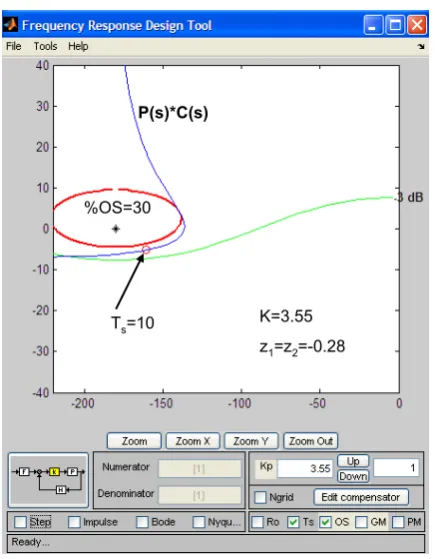
[image:5.595.312.542.96.285.2]A snapshot of the graphical user interface in FRtool and controller parameters are given in Figure-9.
Figure-9. FRtool design for .
[image:5.595.60.278.172.452.2]Both PID controllers have the specifications: % = and 𝑠= second. For the KCR auto-tuner, the specification for settling time gives 𝜔 = . rad/s it follows𝑀 = . ,𝜑 = ° and 𝑀 = °. The controller parameters are given in Table-2 for both controllers. Figure-9 shows the design of the PID controller using the knowledge of the transfer function of the process, by means of FRtool.
Table-2. Controller parameters for .
PID 𝑲𝒑 𝑻𝒊 𝑻𝒅
FRtool
KCR 1.98 2.74 7.14 6.33 1.78 1.58
Figure 10 shows the comparison between the
‘best’ design possible (FRtool) and the KCR auto-tuner. Once again the proposed PID auto-tuner can provide similar results to a PID controller designed based on the model of the process.
Figure-10. Closed loop step responses for the two
PID controllers.
[image:5.595.322.534.427.597.2]Figure-11 depicts the Bode plot, validating the specification crossover frequency around 0.7 rad/s. Due to the fact that this is an exotic system, the bandwidth frequency has to be seen from the phase plot, whereas the definition of 𝑀 is used to find the phase margin -110°, corresponding to +250° in the Bode plot. From here it follows that the bandwidth frequency is about 1.1 rad/s.
Figure-11. Validation of controller in open loop
(SYS*PID) and closed loop for the specified crossover frequency (phase margin) and bandwidth frequency
(settling time) for
From these examples, which are by far much more difficult than systems closer to a second order approximation, it can be concluded that the PID auto-tuner performs comparable with a PID controller tuned based on the knowledge of the transfer function.
3.3 Conclusions
The development and validation of a generally valid, specifications-based, PID auto-tuner have been presented in this paper. The PID controller has been tested successfully on two illustrative examples: i) a double
%OS=30
T
s=10
K=3.55
z
1=z2=-0.28
P(s)*C(s)
%OS=30
T
s=10
K=3.55
z
1=z2=-0.28
P(s)*C(s)
0 5 10 15 20 25 30 -0.4
-0.2 0 0.2 0.4 0.6 0.8 1 1.2 1.4 1.6
Time (s)
FRtool KCR
-20 -10 0 10 20
M
a
g
n
itu
d
e
(
d
B
)
10-2 10-1 100 101 102
-360 -180 0 180 360
P
h
a
s
e
(
d
e
g
)
Bode Diagram
Frequency (rad/sec)
SYS*PID closed-loop
BW
[image:5.595.51.287.597.642.2]integrator in the loop and ii) a double integrator, with time delay and non-minimum phase dynamics. The simulation results were promising and ongoing research is focused to apply this PID auto-tuner on several real-life applications.
REFERENCES
[1] D. Bernstein & L. Bushnell. 2002. The history of control: from idea to technology. IEEE Control Systems Magazine. 22(2): 21-23.
[2] K. J., Åström & T. Hägglund. 1995. PID Controllers: Theory, Design and Tuning. Instrument Society of America, Research Triangle Park, NC, USA.
[3] A., Leva, C. Cox & A. Ruano. 2002. Hands-on PID auto-tuning: a guide to better utilization. IFAC Professional Brief.
[4] K.J., Åström & T. Hägglund. 1984. Automatic tuning of simple regulators with specifications on phase and amplitude margins. Automatica. 20: 645-651.
[5] C.C., Hang, K.J. Åström& W.K. Ho. 1991. Refinements of the Ziegler-Nichols Tuning Formula. In: IEE Proc. Design, Control Theory and Appl. 138: pp. 111-118.
[6] K.J., Åström, C.C. Hang, P. Persson & W.K. Ho. 1992. Towards intelligent PID control. Automatica. 28: 1-9.
[7] J. G. Ziegler & N.B. Nichols. 1942. Optimum settings for automatic controllers. Transactions of ASME. 64: 759-768.
[8] T. S. Schei. 1994. Automatic tuning of PID controllers based on transfer function estimation. Automatica. 30: 1983-1986.
[9] C. Scali, G. Marchetii & D. Semino. 1999. Relay with additional delay for identification and auto-tuning of completely unknown processes. Ind. Eng. Chem. Res. 38: 1987-1997.
[10]R. De Keyser, C. Ionescu. 2010. A Comparative Study of Three Relay-based PID Auto-tuners. Accepted for presentation at the IASTED International Conference on Control and Applications, which will be held July 15, 2010 to July 17, 2010, in Banff, Alberta, Canada.
[11]N.S. Nise. 2007. Control systems engineering, 4th ed., Wiley India Pvt. Ltd.